Geostatistical Reconstruction of Atmospheric Refractivity Fields Using Universal Kriging

Abstract

Atmospheric refractivity governs the propagation behavior of electromagnetic waves in the lower troposphere. Accurate spatial characterization of this parameter is essential for optimizing communication, radar, and navigation systems. This study presents a geostatistical framework for generating high-resolution refractivity maps using Universal Kriging (UK) applied to meteorological observations from a dense network of automatic weather stations in the Galician region (NW Spain). The methodology explicitly models the non-stationary vertical structure of the atmosphere by decomposing the refractivity field into a deterministic altitude-dependent drift and a stochastic residual component characterized by an exponential variogram. Validation, performed using independent test stations bounding the regional vertical profile, demonstrates that the UK approach significantly outperforms Ordinary Kriging (OK). UK not only reduces mean errors and improves linear agreement, but critically minimizes systematic bias and extreme outlier occurrences ($P_{95}$). Beyond accurate spatial interpolation, the dynamically estimated vertical drift retrieves the macroscopic refractivity gradient, serving as a direct, real-time diagnostic tool to classify anomalous radio-frequency (RF) propagation regimes (e.g., super-refraction and ducting) and supporting robust decision-making in complex topographies.

1. Introduction

The propagation of electromagnetic waves in the troposphere is strongly influenced by local atmospheric conditions, which govern the spatial and temporal variability of the refractive index. This behavior is quantitatively described through atmospheric refractivity, a parameter derived from meteorological variables such as pressure, temperature, and relative humidity [1]. Accurate knowledge of the spatial distribution of refractivity is therefore essential not only for meteorology but also for the design, performance assessment, and optimization of radio-frequency (RF) communication, radar, and navigation systems.

In meteorology, a reliable characterization of near-surface refractivity is crucial for properly initializing numerical weather prediction (NWP) models [2,3] and for the identification and short-term forecasting of severe storm development, which is often associated with sharp spatial refractivity gradients [4]. In RF applications, refractivity information is required to solve the Parabolic Equation (PE), a widely used computational method for simulating electromagnetic wave propagation in complex environments [5,6]. Moreover, refractivity plays a key role in predicting shadow-fading behavior and enabling accurate path-loss (PL) modeling in wireless channels, determining the attenuation experienced by a signal as it travels through the atmosphere and interacts with terrain features and man-made structures [7,8]. In the context of next-generation cellular networks, local refractivity profiles are increasingly relevant for assessing inter-cell interference risks caused by anomalous long-distance ducting propagation [9]. In radar systems, accurate knowledge of refractivity is also essential because beam bending induced by atmospheric stratification affects target detection and tracking performance [10,11].

Furthermore, precise characterization of the refractive index field is of paramount importance in satellite navigation and Earth observation applications. In Global Navigation Satellite Systems (GNSSs), the tropospheric delay caused by signal refraction in the neutral atmosphere represents a major source of positioning error, particularly affecting the vertical component [12,13]. Similarly, in Interferometric Synthetic Aperture Radar (InSAR), spatiotemporal variations in atmospheric moisture induce phase shifts that appear as noise in deformation interferograms [14,15]. Reliable knowledge of the near-surface refractivity field enables the mitigation of these atmospheric artifacts, thereby facilitating the separation of true geophysical ground displacements from atmospheric effects [16].

Traditionally, refractivity is estimated from point-wise measurements obtained at meteorological stations. However, the sparse and irregular distribution of these networks limits the ability to reconstruct continuous refractivity fields over large or topographically complex regions. Spatial interpolation techniques offer a solution to this limitation by exploiting the geospatial correlation of the physical parameters, enabling the generation of reliable maps even in areas with low station density [17,18].

Among the various interpolation methods, Kriging is widely recognized for its geostatistical foundations and its ability to provide the Best Linear Unbiased Predictor (BLUP) [19,20,21,22,23]. Standard approaches, such as Ordinary Kriging (OK), rely on the assumption of stationarity, where the mean and variance of the variable are assumed to be constant across the domain [24]. However, atmospheric refractivity exhibits strong systematic dependence on altitude (vertical gradient), which violates the stationarity assumption in regions with significant topographic relief. Ignoring this vertical trend can lead to substantial prediction errors when interpolating between stations at different elevations.

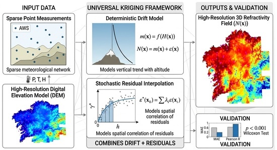
To address this challenge, this study demonstrates the operational implementation of Universal Kriging (UK) to generate high-resolution spatial maps of atmospheric refractivity. While the mathematical framework of UK is well-established, its application to a high-density Automatic Weather Station (AWS) network in a topographically complex coastal–mountainous region bridges the gap between geostatistical theory and real-world meteorological operations. The proposed approach explicitly models the non-stationary mean as a function of elevation, separating the deterministic vertical trend from the stochastic residuals, which are subsequently characterized by an exponential variogram to capture the inherent spatial roughness of the boundary layer [24,25]. The spatial variability of refractivity in the study region is analyzed, and the accuracy of the interpolated fields is rigorously evaluated against standard spatial interpolation techniques. The resulting maps provide a physically consistent representation of the lower atmosphere, directly supporting the development of robust wave propagation models for engineering and meteorological applications.

The remainder of this paper is organized as follows. Section 2 introduces the theoretical background of atmospheric refractivity, detailing its relationship with meteorological parameters and the calculation of vertical gradients. Section 3 describes the applied geostatistical framework, focusing on the UK formulation, the practical modeling of the deterministic trend using elevation data, and the variographic analysis of residuals. 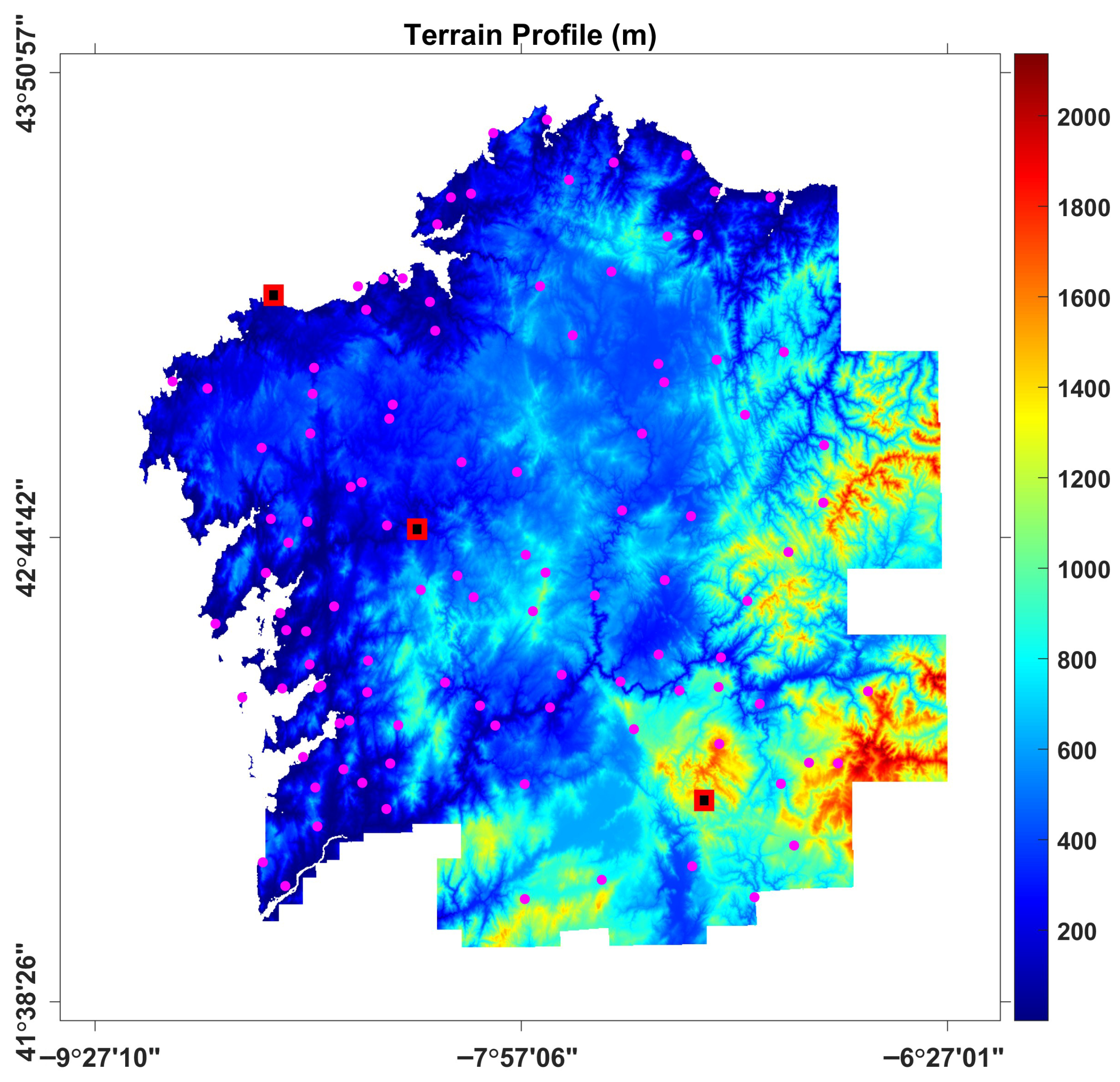Section 4 presents the specific study scenario and the experimental dataset, including the description of the Galician region, the Digital Elevation Model (DEM), and the meteorological station network. Section 5 presents the implementation results, validating the generated high-resolution maps against standard techniques using independent test stations. Section 6 discusses the physical and operational implications of the findings, providing a comprehensive analysis of the macroscopic refractivity gradients. Finally, Section 7 summarizes the main conclusions and future lines of research.

2. Refractivity from Automatic Weather Stations

2.1. Theoretical Background

Atmospheric refractivity quantifies the deviation of the refractive index of air from unity. It is formally defined as [26]:

$$N=(n-1)\times {10}^6,$$

(1)

where n is the refractive index of air and N is the radio refractivity, expressed in N-units. Since n in the troposphere is very close to 1, the factor 10⁶ provides a practical scale for expressing small spatial and temporal variations.

For radio frequencies, refractivity is a function of meteorological parameters, specifically pressure, temperature, and water vapor pressure, given by the Smith–Weintraub equation [1]:

$$N=77.6{\displaystyle \frac{P}{T}}+3.73\times {10}^5{\displaystyle \frac{e}{T^2}},$$

(2)

where P is the total atmospheric pressure (hPa), T is the absolute temperature (K), and e is the partial pressure of water vapor (hPa). The first term ($77.6P/T$) depends on the total atmospheric pressure, which is the sum of the dry air pressure and the water vapor pressure. Although it incorporates e, this component is conventionally referred to in radio engineering literature as the dry term (or hydrostatic term), primarily reflecting air density. The second term ($3.73\times {10}^{5}e/T^2$) accounts for the wet term, driven by the dipole moment of water vapor molecules.

The partial water vapor pressure e is derived from the relative humidity ($RH$ [%]) and the saturation vapor pressure ($e_s$) as:

$$e={\displaystyle \frac{RH}{100}} e_s.$$

(3)

The saturation vapor pressure $e_s$ (in hPa) is estimated using the Magnus–Tetens empirical relationship:

$$e_s=6.112\times exp\left({\displaystyle \frac{17.62 T_C}{243.12+T_C}}\right),$$

(4)

where $T_C$ is the air temperature in degrees Celsius. Combining these expressions allows for the direct computation of N from standard meteorological observations.

2.2. Vertical Refractivity Gradient and Propagation Conditions

The vertical variation of refractivity, denoted as $\partial N/\partial z$, governs the bending of electromagnetic waves in the lower atmosphere. Under standard atmospheric conditions, refractivity decreases with height at a rate of approximately 39 N-units/km, resulting in a slight downward bending of radio waves towards the Earth.

Deviations from this standard atmosphere lead to anomalous propagation conditions, which are classified based on the gradient value [1]. Sub-refraction occurs when $\partial N/\partial z>-39$ N-units/km; in this regime, the wave bends less than usual, effectively reducing the radio horizon. Conversely, super-refraction corresponds to gradients typically between $-157$ and $-75$ N-units/km, causing the wave to bend significantly towards the ground and extending the horizon. In extreme cases where $\partial N/\partial z<-157$ N-units/km, ducting phenomena occur, where the wave becomes trapped within an atmospheric layer and can propagate over vast distances. Understanding these regimes is critical for assessing coverage and potential interference.

In the context of UK, this large-scale vertical variation is approximated as a linear drift:

$$N\left(z\right)\approx N_0+{\displaystyle \frac{\partial N}{\partial z}}·z,$$

(5)

where $N\left(z\right)$ is the refractivity at elevation z (km), $N_0$ is the projected refractivity at sea level, and $\partial N/\partial z$ represents the regional vertical gradient.

While the full atmospheric column exhibits an exponential refractivity decay due to hydrostatic pressure, a linear drift provides a robust and physically consistent approximation within the lowest few kilometers of the troposphere. Crucially for spatial interpolation, this linear parameterization guarantees mathematical stability within the Kriging system, avoiding the overfitting and numerical artifacts often introduced by higher-order non-linear trends across irregular sensor networks.

2.3. Refractivity Derived from Automatic Weather Stations

This study utilizes measurements from a network of ground-based meteorological stations distributed across the study region. Each station records atmospheric pressure (P), temperature ($T_C$), and relative humidity ($RH$) at 10-min intervals. These observations are processed to compute atmospheric refractivity (N) using Equations (2)–(4).

Figure 1 and Figure 2 present the time series of the raw meteorological variables and the corresponding derived refractivity for a representative weather station (Rus, coordinates: ${43}^{\circ }{09}^{\prime }{22}^{″} \mathrm{N}$, $8^{\circ }{41}^{\prime }{07}^{″} \mathrm{W}$, 161 m above sea level). As expected, short-term refractivity fluctuations are predominantly driven by variations in water vapor pressure, followed by temperature. In contrast, while total atmospheric pressure dominates the baseline magnitude of N (via the dry term), its minimal temporal variance exerts a negligible influence on these high-frequency refractivity dynamics.

Simple Linear Model (Ordinary Least Squares)

To estimate the vertical refractivity gradient, an Ordinary Least Squares (OLS) regression is applied to the elevation-refractivity pairs $(z_i,N_i)$ extracted from the meteorological network. Assuming a macroscopic linear dependence of refractivity on height within the lower troposphere, the model is defined as:

$$N_i={\beta }_0+{\beta }_1{z}_i+{\epsilon }_i,$$

(6)

where $N_i$ is the refractivity at station i, $z_i$ is the station height (expressed in km), ${\beta }_0$ represents the projected refractivity at sea level, ${\beta }_1$ is the vertical refractivity gradient, and ${\epsilon }_i$ are the residuals assumed to be independent and identically distributed with zero mean.

The coefficients ${\beta }_0$ and ${\beta }_1$ are obtained by minimizing the sum of squared residuals:

$$\underset{{\beta }_0,{\beta }_1}{min}\sum _{i=1}^n{\left(N_i-{\beta }_0-{\beta }_1{z}_i\right)}^2,$$

(7)

yielding the well-known OLS estimators:

$$\begin{array}{cc}\hfill {\widehat{\beta }}_1& ={\displaystyle \frac{{\sum }_{i=1}^n(z_i-\overline{z})(N_i-\overline{N})}{{\sum }_{i=1}^n{(z_i-\overline{z})}^2}},\hfill \end{array}$$

(8)

$$\begin{array}{cc}\hfill {\widehat{\beta }}_0& =\overline{N}-{\widehat{\beta }}_1 \overline{z},\hfill \end{array}$$

(9)

where $\overline{N}$ and $\overline{z}$ denote the sample means of refractivity and height, respectively.

The fitted gradient ${\widehat{\beta }}_1$ is subsequently used to construct the deterministic drift term in the UK formulation, while the residuals:

$${\widehat{\epsilon }}_i=N_i-{\widehat{\beta }}_0-{\widehat{\beta }}_1{z}_i$$

(10)

represent the stochastic component required for the empirical semivariogram computation.

3. Geostatistical Interpolation Using Universal Kriging

3.1. Kriging Interpolation

Kriging is a geostatistical interpolation method that predicts the value of a variable at unsampled locations by modeling the spatial correlation structure of observed data. Given a set of n observations ${\left\{N\left({\mathbf{x}}_i\right)\right\}}_{i=1}^n$, the Kriging estimator at an unsampled location ${\mathbf{x}}_0$ is expressed as:

$$\widehat{N}\left({\mathbf{x}}_0\right)=\sum _{i=1}^n{\lambda }_i N\left({\mathbf{x}}_i\right),$$

(11)

where ${\lambda }_i$ are weights determined by minimizing the estimation variance under the constraint of unbiasedness. The spatial dependence among points is quantified using the empirical semivariogram:

$$\gamma \left(h\right)={\displaystyle \frac{1}{2M\left(h\right)}}\sum _{i,j\in S\left(h\right)}{\left[N\left({\mathbf{x}}_i\right)-N\left({\mathbf{x}}_j\right)\right]}^2,$$

(12)

where $h=|{\mathbf{x}}_i-{\mathbf{x}}_j|$ is the lag distance, and $M\left(h\right)$ represents the number of point pairs separated by distance h.

To mathematically define how this spatial correlation decays with distance, a continuous theoretical model (such as the spherical, exponential, or Gaussian model) is fitted to the empirical semivariance [24,25]. The evaluated values from this continuous theoretical semivariogram are then used to populate the spatial covariance matrices of the Kriging system, both between the sampled observation points and between the observations and the target prediction location ${\mathbf{x}}_0$. Solving this linear system directly yields the optimal spatial weights ${\lambda }_i$.

3.2. Universal Kriging with Altitude-Dependent Drift

UK extends OK by incorporating a deterministic drift alongside stochastic residuals. In this study, the deterministic drift accounts for the systematic variation of refractivity with elevation. This is derived from the vertical refractivity gradient concept described in Section 2.3:

$$m\left(\mathbf{x}\right)=N_0+{\beta }_1 z\left(\mathbf{x}\right),$$

(13)

where $N_0$ is the intercept, ${\beta }_1$ corresponds to the vertical refractivity gradient ($\partial N/\partial z$), and $z\left(\mathbf{x}\right)$ is the elevation at location $\mathbf{x}$.

This formulation allows the interpolation to capture large-scale refractivity trends associated with altitude, while the residual component $\epsilon \left(\mathbf{x}\right)$ accounts for local spatial fluctuations:

$$N\left(\mathbf{x}\right)=m\left(\mathbf{x}\right)+\epsilon \left(\mathbf{x}\right).$$

(14)

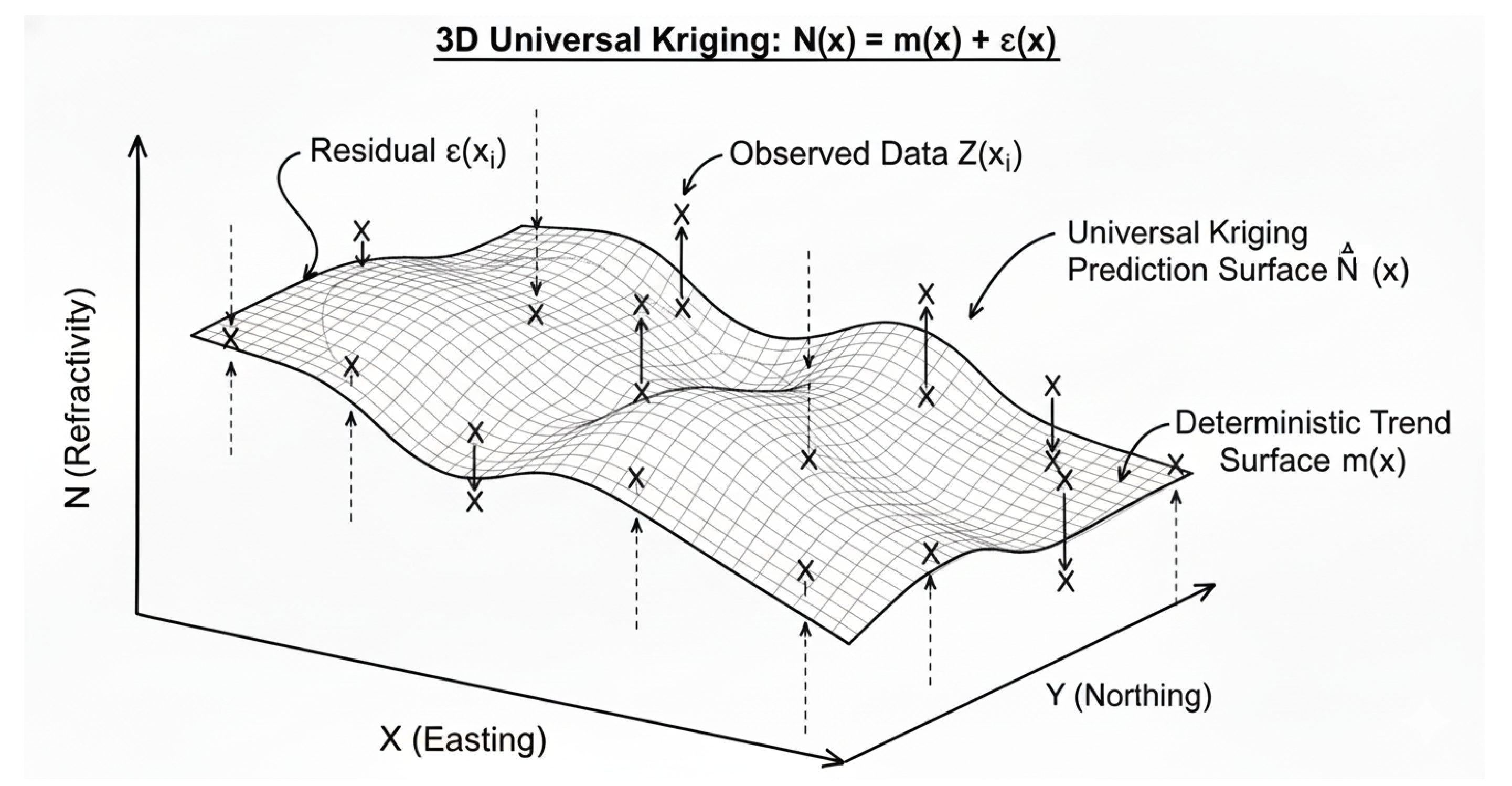
To better visualize this decomposition, Figure 3 presents a schematic 3D representation of this geostatistical decomposition. The deterministic trend, denoted as $m\left(\mathbf{x}\right)$, is depicted as a smooth surface that captures the systematic variation of refractivity driven by the vertical gradient ${\beta }_1$. The vertical deviations of the observed data points from this macroscopic trend constitute the stochastic residuals $\epsilon \left(\mathbf{x}\right)$. The final UK prediction surface is synthesized by summing this deterministic drift and the spatially interpolated residuals, guaranteeing the preservation of both the regional atmospheric physics and the local statistical anomalies.

Consequently, the UK estimator at ${\mathbf{x}}_0$ is defined as a linear combination of the observed data, subject to constraints that filter the drift:

$$\widehat{N}\left({\mathbf{x}}_0\right)=\sum _{i=1}^n{\lambda }_i N\left({\mathbf{x}}_i\right).$$

(15)

To ensure unbiasedness in the presence of the drift, the Kriging weights must satisfy the following constraints:

$$\sum _{i=1}^n{\lambda }_i{f}_k\left({\mathbf{x}}_i\right)=f_k\left({\mathbf{x}}_0\right) \mathrm{for} k=0,\dots ,K$$

(16)

where $f_k\left(\mathbf{x}\right)$ represent the basis functions of the deterministic drift. In our specific linear altitude-dependent model, the drift order is $K=1$, meaning the only basis functions utilized in the Kriging system are $f_0\left(\mathbf{x}\right)=1$ (accounting for the constant intercept) and $f_1\left(\mathbf{x}\right)=z\left(\mathbf{x}\right)$ (accounting for the elevation).

3.3. Semivariogram Estimation

The spatial structure of the residual component $\epsilon \left(\mathbf{x}\right)$ is characterized through semivariogram analysis. To identify the optimal correlation model, empirical semivariograms were computed and fitted to several theoretical functions (spherical, Gaussian and exponential). The automated fitting procedure utilizes Weighted Least Squares (WLS) to prioritize the accurate modeling of short-lag correlations, which are mathematically dominant in determining the final interpolation weights.

To compute the empirical semivariogram, the spatial domain is dynamically parameterized to ensure statistical robustness. The maximum lag distance ($h_{max}$) is restricted to half the maximum diagonal extent of the active AWS network, which corresponds to approximately $1.4^{\circ }$ (roughly 155 km). This domain is then strictly partitioned into 8 discrete lag bins. This specific discretization yields a dynamic lag bin width of approximately $0.{175}^{\circ }$ (∼19 km), a scale that guarantees a massive population of point-pairs within each bin to suppress erratic variance spikes, while retaining the necessary spatial granularity to resolve short-range correlations.

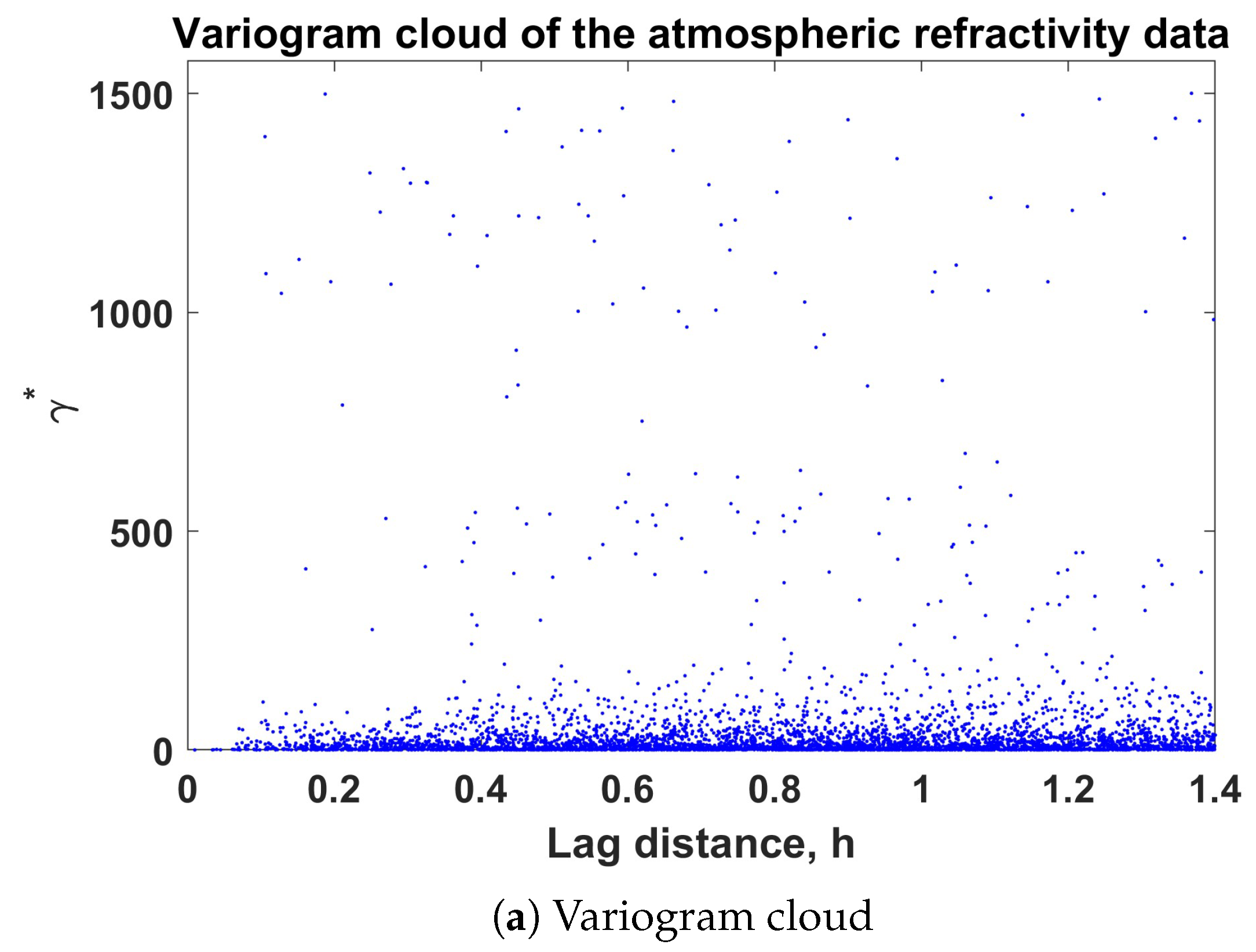
To explicitly demonstrate the spatial correlation structure of the refractivity fields, Figure 4a presents an example of the raw variogram cloud, where each point represents the semivariance (${\gamma }^{*}$) of a unique station pair against its spatial separation distance (h), up to a maximum reliable range of 1.4^∘. Due to the high dispersion inherent in the unbinned data, applying a lag distance classification is necessary to compute a stable spatial structure. 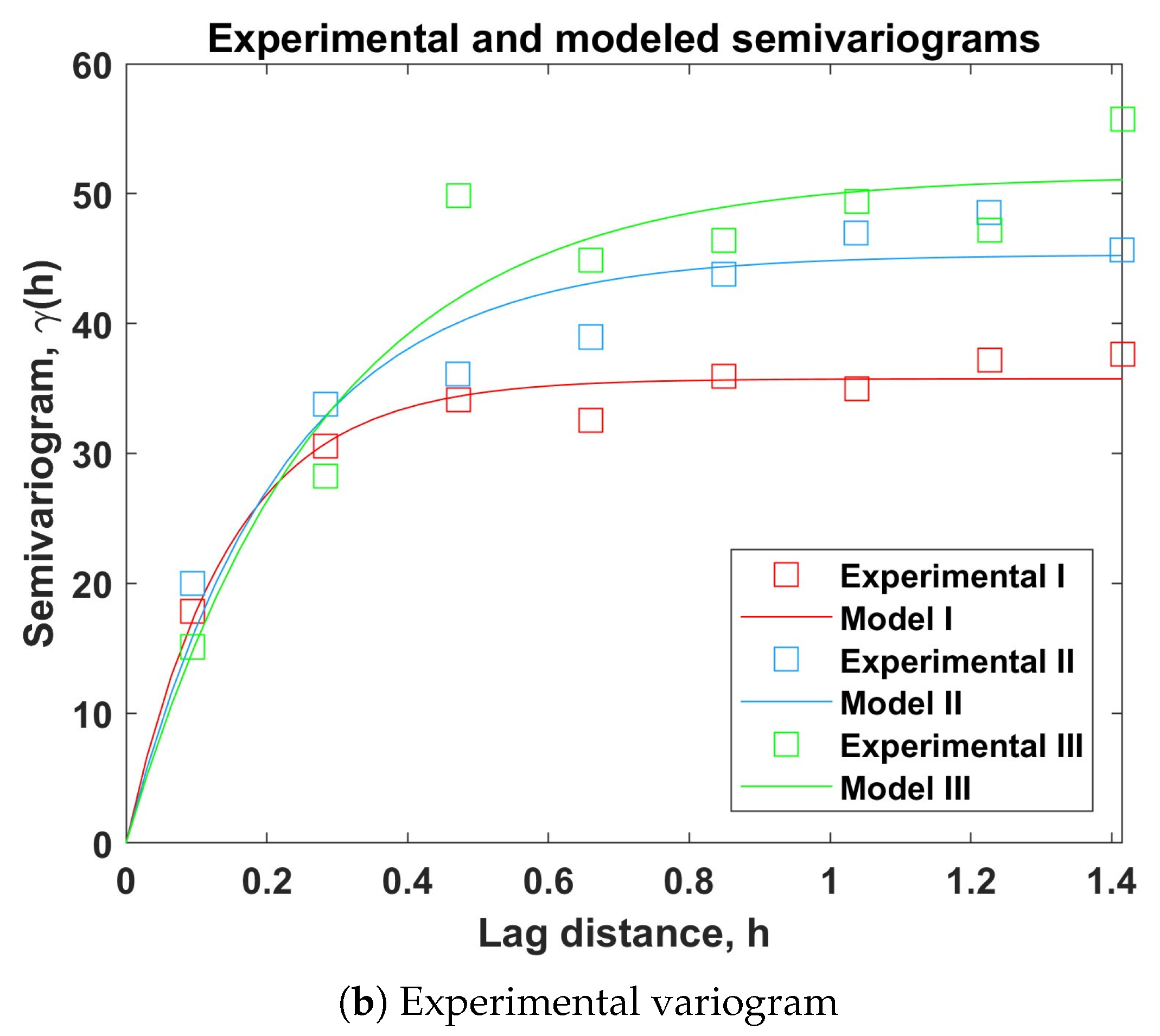Consequently, Figure 4b illustrates the resulting binned experimental semivariograms alongside their dynamically fitted exponential models as a function of h (expressed in decimal degrees) for three representative atmospheric scenarios. These correspond to standard propagation conditions (Experimental I), sub-refractive conditions (Experimental II), and super-refractive conditions (Experimental III), which will be analyzed in detail in Section 5. This comparison visually demonstrates the algorithm’s robustness and adaptability across fundamentally different atmospheric stability regimes.

To robustly justify the theoretical model selection, spherical, Gaussian, and exponential functions were systematically evaluated over the dataset using the WLS optimization algorithm. The WLS objective function heavily penalizes deviations at short lag distances by applying a weighting factor of $w=1/h^2$ (normalized to sum to unity, acting as a weighted mean squared error), ensuring maximal fidelity near the origin where Kriging weights are most sensitive.

The quantitative analysis definitively identified the exponential model as the optimal fit, yielding an average WLS error of 4.42, outperforming both the spherical (5.02) and Gaussian (5.88) models. Beyond its numerical superiority, the exponential model exhibits a linear behavior near the origin, correctly characterizing the spatial roughness and abrupt gradient transitions typical of boundary layer refractivity over complex topography, unlike the artificially smooth Gaussian assumption. Consequently, the exponential model was established as the standard theoretical semivariogram. The optimized structural parameters yielded a mean practical range of $0.{34}^{\circ }$, a sill of 37.44, and a representative nugget effect of 12.03, which accurately captures inherent micro-scale atmospheric variability and instrumental noise. The resulting variogram parameters (nugget, sill, and range) define the spatial covariance matrix required to compute the Kriging weights.

Although coastal–mountainous regions can induce anisotropic physical dynamics (e.g., directional correlations aligned with coastlines or valleys), an isotropic spatial covariance model is strictly enforced in this framework to guarantee continuous algorithmic stability. In a fully automated system computing high-frequency epochs, dynamically partitioning the AWS network into directional angular bins significantly dilutes the available point pairs per bin. This sparsity compromises statistical robustness, leading to noisy empirical variograms and unstable theoretical fits that risk generating non-positive-definite covariance matrices. Consequently, the robust isotropic exponential model ensures continuous, reliable Kriging system resolution without requiring manual intervention. Exploring dynamically adaptive anisotropic models remains a valuable objective for future research, provided network density permits robust directional fitting in real-time.

3.4. Implementation Steps

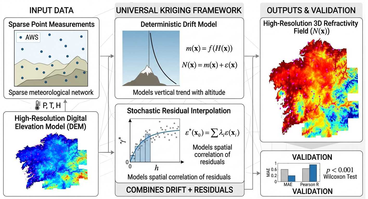
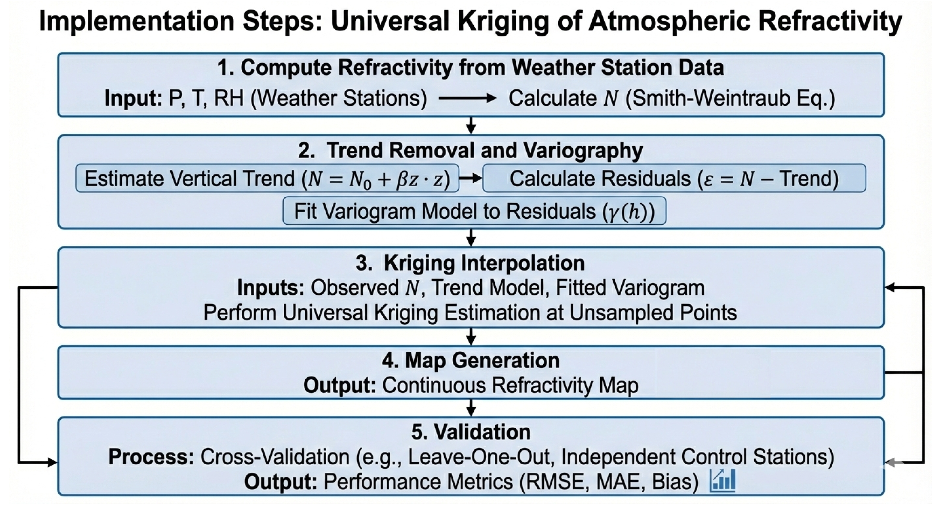
The operational workflow of the proposed framework, illustrated in Figure 5, is summarized as follows:

1.

Compute Refractivity from Weather Station Data: Convert the raw meteorological observations obtained from the automatic weather stations into atmospheric refractivity values using Equations (2)–(4).

2.

Trend Removal and Variography: Estimate the macroscopic vertical trend to isolate the stochastic residuals. Calculate the empirical semivariogram of these residuals and fit the optimal continuous theoretical model (i.e., the exponential model) to mathematically describe the spatial correlation structure.

3.

Kriging Interpolation: Estimate refractivity (N) at unsampled grid locations using UK, solving the spatial system of equations that strictly enforces both the variogram covariance and the altitude-dependent drift constraints.

4.

Map Generation: Produce continuous, high-resolution spatial maps of refractivity over the study area.

5.

Validation: Evaluate interpolation performance using independent test stations to compare predicted and observed values, comprehensively quantifying accuracy via mean errors (RMSE, MAE), systematic deviations (bias), and extreme outlier occurrences ($P_{95}$).

All data processing and spatial modeling, including the automated UK interpolations, were implemented natively in MATLAB (version R2025b). The dynamic computation of the empirical semivariograms and the subsequent WLS bounded optimization for the theoretical model fitting were executed utilizing the geostatistical functions provided by [27].

This methodology provides a statistically rigorous framework for generating high-resolution refractivity maps from sparse meteorological networks. By explicitly modeling the vertical deterministic structure, it enables a significantly more accurate characterization of spatial refractivity variability and radio propagation conditions compared to standard techniques (such as OK or Inverse Distance Weighting (IDW)) that inherently fail to account for topographic elevation.

4. Scenario and Data

4.1. Study Area

The study area comprises the Galician region (NW Spain), covering approximately 30,000 km². The region is characterized by complex orography, with elevations ranging from sea level to mountainous terrain (see Figure 6). Topographic information was obtained from a DEM provided by the National Geographical Institute [28], with a spatial resolution of 25 m. This high-resolution DEM provides the continuous surface elevation $z\left(\mathbf{x}\right)$ required to model the altitude-dependent drift within the UK formulation.

4.2. Datasets

The analysis relies on meteorological observations from a regional network of 109 automatic weather stations irregularly distributed across the study area (represented as magenta circles in Figure 6). The network provides measurements of atmospheric pressure (P) [hPa], air temperature ($T_C$) [^∘C], and relative humidity ($RH$) [%] at 10-min intervals [29].

The dataset spans the period from 00:00 UTC on 10 August 2018 to 23:50 UTC on 25 September 2018. This corresponds to a total of 6768 temporal epochs (time steps) for each of the 109 stations, providing a high-resolution temporal basis for the spatial analysis.

To rigorously evaluate the spatial interpolation accuracy, a targeted hold-out validation strategy was implemented using strategically selected independent test stations. While global techniques like Leave-One-Out Cross-Validation (LOOCV) provide an averaged performance metric across the entire domain, they often mask localized errors in complex topography by smoothing out the results [30,31,32]. Instead, utilizing a static, independent test set strictly positioned at distinct elevations enables a highly critical assessment of the model’s ability to reconstruct the vertical refractivity drift without the averaging effects of global cross-validation.

Predictive accuracy is quantified by computing the RMSE and MAE between the Kriging predictions and the empirical reference values at these test locations. Furthermore, to explicitly address systematic deviations and extreme interpolation anomalies, the mean bias and the 95th percentile of the absolute error ($P_{95}$) are evaluated. Detailed time-series analyses are presented for three representative test stations (highlighted as black and red squares in Figure 6) purposely chosen to bound the regional vertical profile: a sea-level station in the northeast, a mid-elevation station (121 m) in the central plateau, and a high-elevation mountain station (1026 m) in the southwest.

While a larger spatial hold-out set might conventionally capture more horizontal variability, restricting the exclusion to three specific vertical probes prevents the artificial degradation of the operational network. Retaining 106 stations maximizes the spatial density required to maintain the stability of the empirical variogram and the deterministic vertical drift calculation. Furthermore, this limited spatial subset is compensated by immense temporal depth, as these three stations are continuously evaluated at 10-min intervals throughout the entire dataset, generating thousands of independent validation points across dynamic atmospheric conditions.

4.3. Implementation and Reproducibility Details

To ensure the reproducibility of the proposed operational framework and guarantee continuous algorithmic stability, two key implementation phases are strictly enforced: automated data filtering and high-resolution spatial projection.

Prior to computing the surface refractivity, the raw meteorological data stream from the AWS network undergoes an automated Quality Control (QC) process. This protocol applies gross-error filters and physical range limits (e.g., capping relative humidity at 100% and removing non-physical temperature or pressure spikes). Any station reporting anomalous or missing data during a specific 10-min epoch is dynamically excluded for that single time step. Because the empirical variograms and theoretical fits are computed strictly on a per-epoch basis (as parameterized in Section 3), the spatial redundancy of the dense network allows the interpolation algorithm to seamlessly absorb these temporary dropouts without compromising the regional spatial covariance structure.

Following the resolution of the deterministic drift and the Kriging weights, the final continuous output is projected onto a regular, high-resolution 25 m × 25 m spatial grid. This specific resolution is explicitly matched to the underlying DEM [28]. By enforcing this strict grid alignment, the UK framework guarantees that high-frequency topographic variations and their corresponding deterministic effects on the lower tropospheric refractivity field are perfectly preserved in the final macroscopic maps.

5. Results

5.1. Temporal Evolution of the Vertical Refractivity Gradient

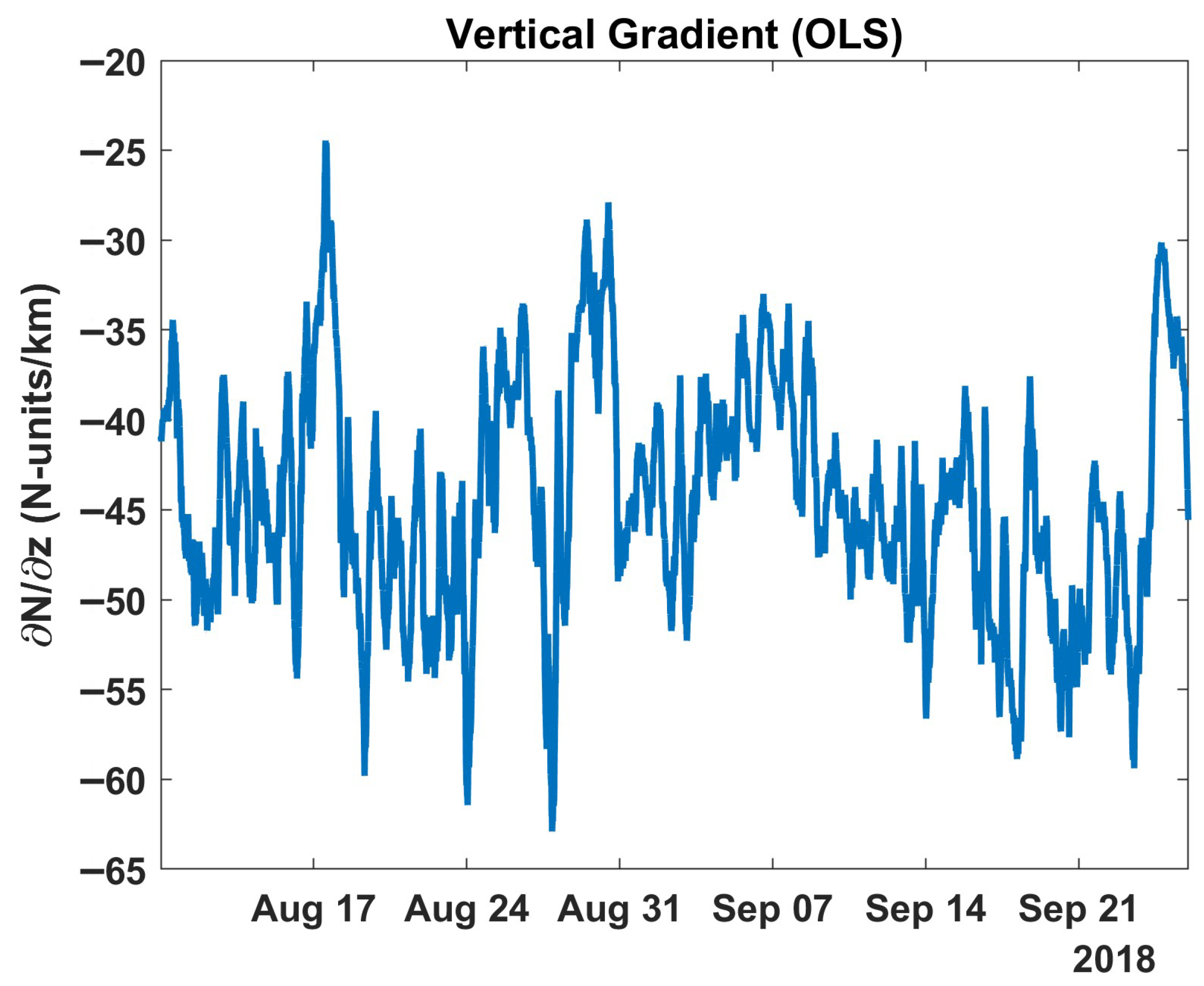
Figure 7 illustrates the temporal evolution of the vertical refractivity gradient estimated from the meteorological station network. For each 10-min interval, the gradient (${\beta }_1$) was computed by fitting the OLS model described in Section 2.3 to the observed refractivity and elevation data.

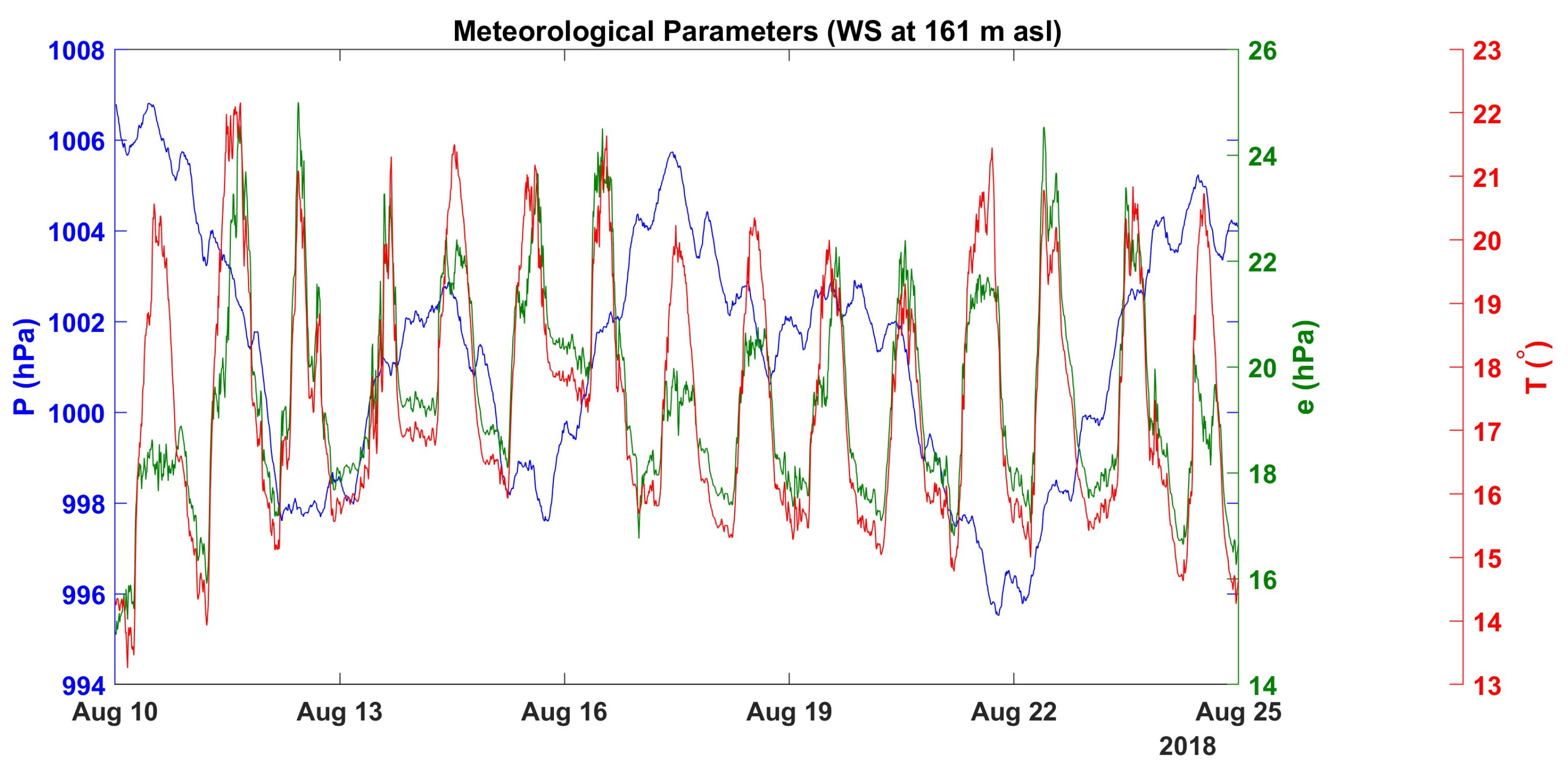
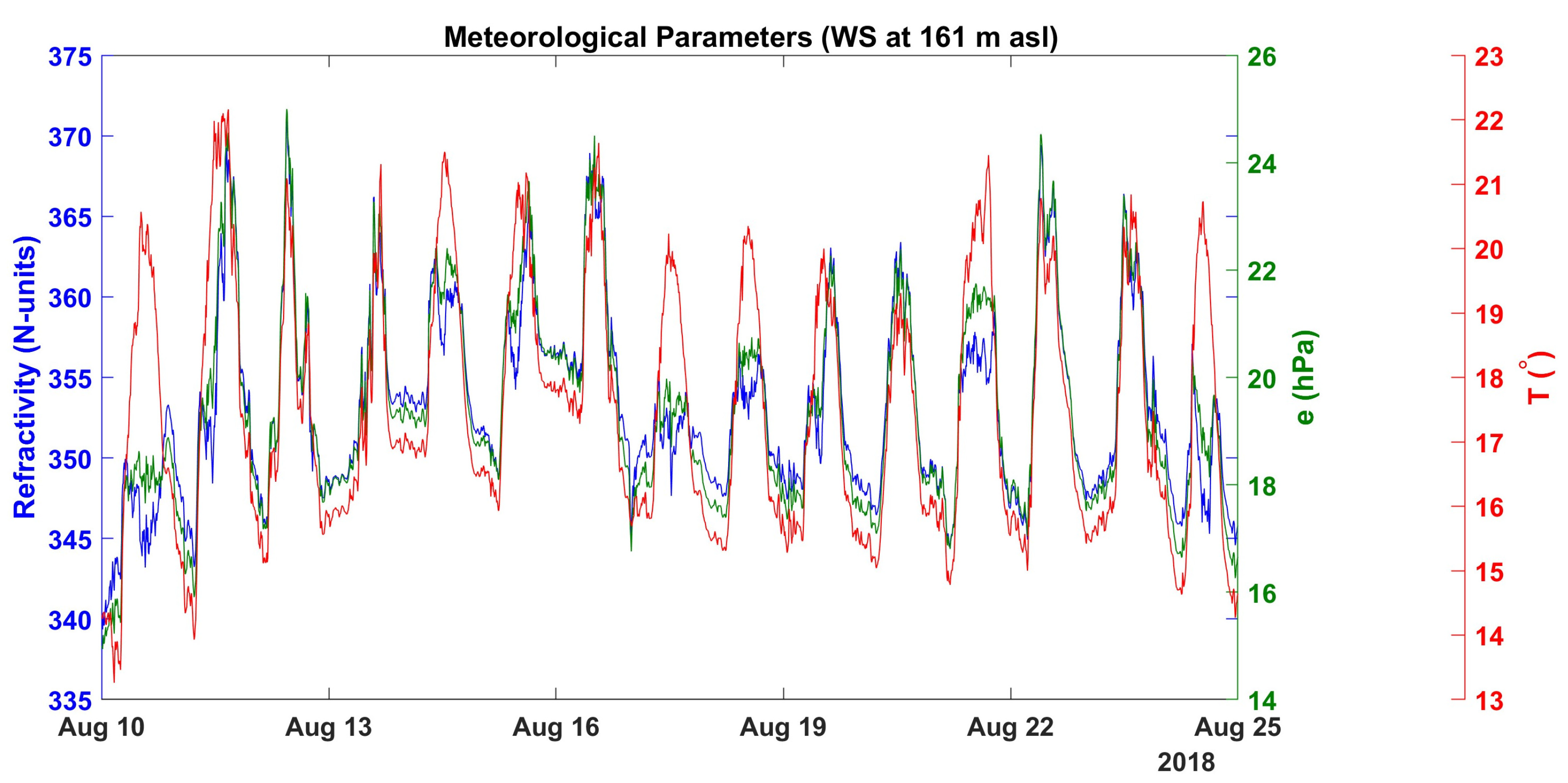
The resulting time series highlights the variability of atmospheric stratification over the study period, driven by diurnal heating–cooling cycles, humidity fluctuations, and synoptic-scale changes in air mass properties (see Figure 1 and Figure 2). Periods exhibiting highly negative gradients (steeper than $-40$ N-units/km) indicate strong refractivity decay with height. These events are typically associated with stable atmospheric conditions, such as nocturnal radiative cooling or the presence of elevated dry layers, which can lead to super-refractive or ducting propagation conditions. Conversely, weaker or near-zero gradients correspond to homogeneous, well-mixed atmospheres, often occurring during daytime convective activity.

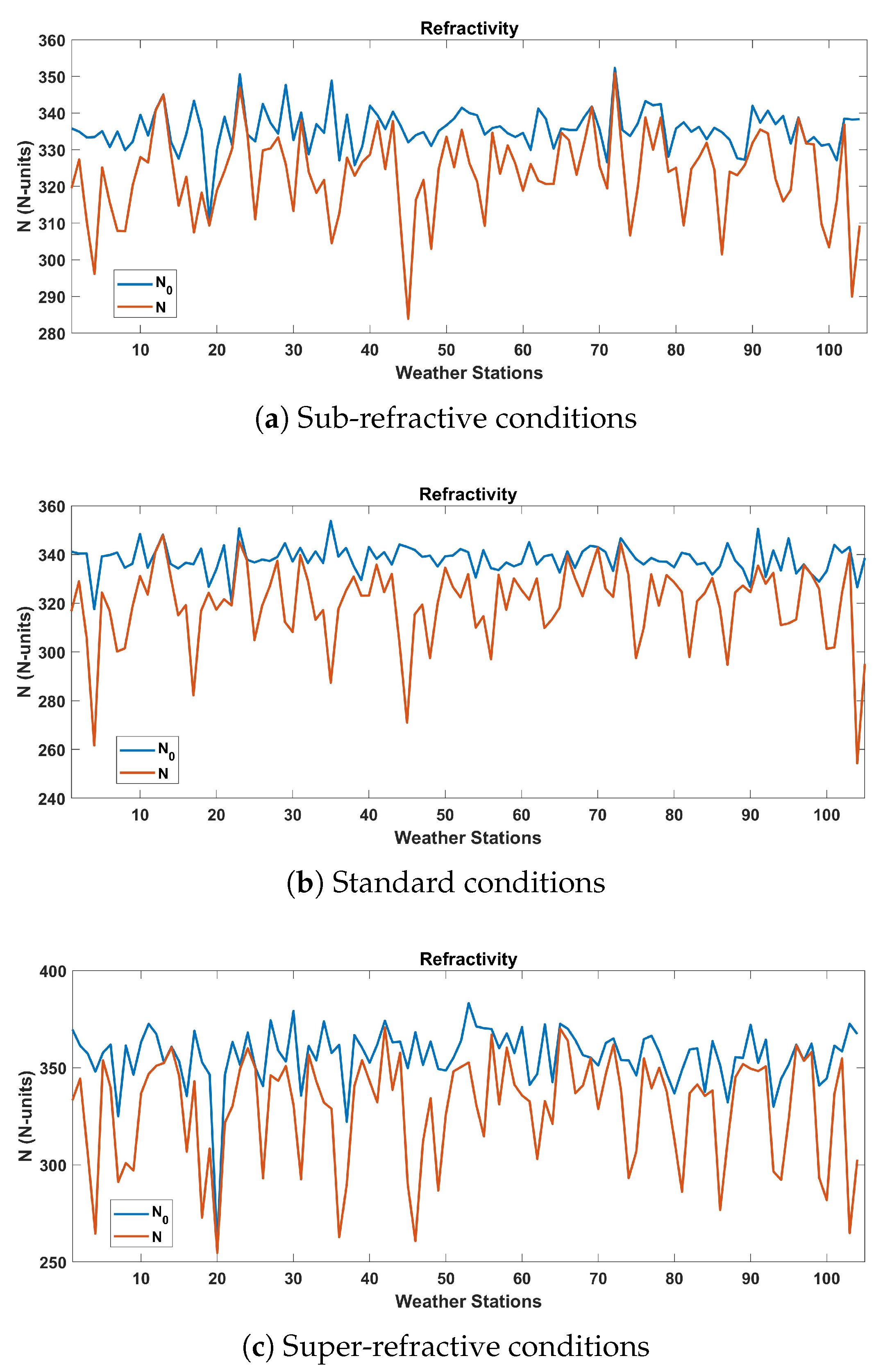
Particular emphasis is placed on three specific epochs chosen to represent distinct propagation regimes. The most pronounced sub-refractive conditions ($-25$ N-units/km) and super-refractive conditions ($-62$ N-units/km) were observed on 17 August at 14:00 UTC and 27 August at 21:50 UTC, respectively. Additionally, a representative case of standard conditions ($-40$ N-units/km) is identified on 18 August at 04:30 UTC.

Figure 8 details the behavior of the network for these three scenarios. The orange line represents the raw surface refractivity (N) derived at each station, while the blue line shows the corresponding sea-level refractivity ($N_0$), obtained by correcting the raw values using the estimated vertical gradient for that epoch ($N_0\approx N-{\beta }_{1}z$). This quantity is crucial as it represents the de-trended field used to compute the residuals prior to UK estimation. The data clearly demonstrates that the sea-level refractivity exhibits significantly lower spatial variance than the raw surface refractivity. This massive variance reduction confirms that the linear drift model successfully removes the dominant altitude dependence, thereby satisfying the stationarity requirements better than the raw data used in OK.

To optimize for near-real-time nowcasting, this operational framework intentionally processes the high-frequency (10-min) AWS data as a sequence of independent 2D spatial interpolations (a “time-slice” approach) rather than employing a computationally heavy 3D space-time Kriging (ST-Kriging) formulation. This deliberate design choice provides two major operational advantages. First, independent 2D spatial Kriging is computationally highly efficient, allowing for instantaneous map generation as new data packets arrive without the heavy computational burden of 3D covariance matrix inversion. Second, by independently re-estimating the deterministic drift and the residual variogram at each epoch, the model retains maximum responsiveness; it can instantly adapt to rapid, non-stationary mesoscale transitions (e.g., fast-moving weather fronts) without the artificial smoothing lag typical of temporally filtered models. Analysis of the time series confirms that, despite this epoch-wise independence, the inferred geostatistical parameters and the resulting prediction errors remain temporally stable and physically coherent throughout the study period.

Characterizing these temporal dynamics is essential for the UK framework. By explicitly updating the drift term $m\left(\mathbf{x}\right)$ at each time step, the interpolation algorithm adapts to the evolving vertical structure of the troposphere, improving prediction accuracy compared to stationary mean models.

5.2. Spatial Distribution of Refractivity Across Atmospheric Regimes

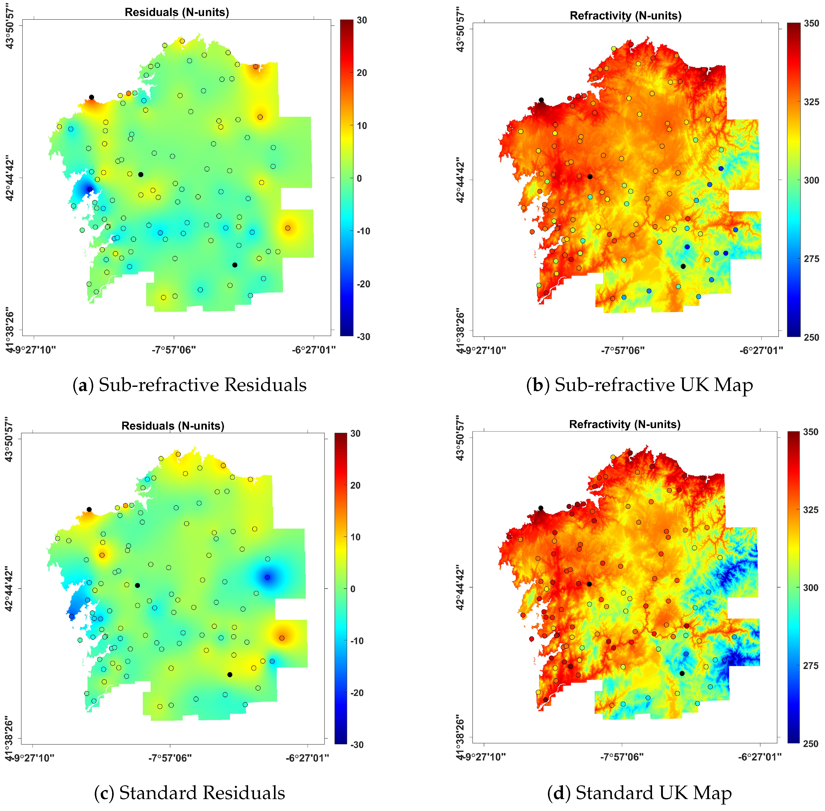
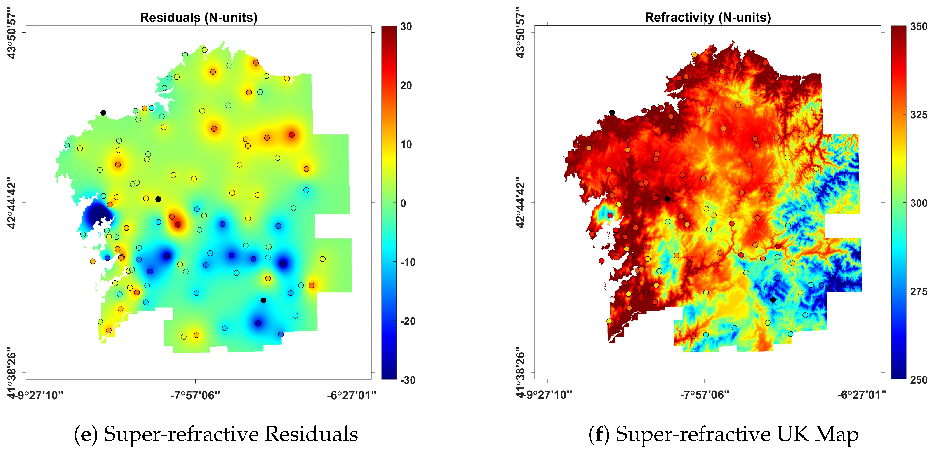
To evaluate the performance of the proposed methodology under varying propagation conditions, Figure 9 presents a spatial comparison of the interpolation results for the three representative atmospheric regimes defined in Section 5.1. The left column displays the isolated stochastic residuals ($\epsilon \left(\mathbf{x}\right)$) obtained after detrending, representing local atmospheric anomalies strictly decoupled from elevation. The right column presents the final high-resolution UK refractivity maps ($\widehat{N}\left(\mathbf{x}\right)$), synthesized by recombining the macroscopic topographic drift and the spatially interpolated residuals.

The spatial signatures within these maps distinctly reflect the underlying atmospheric physics. In sub-refractive situations (top row, Figure 9a,b), the vertical gradient is inherently weaker (less negative), resulting in smaller residual amplitudes and a high degree of spatial homogeneity in the detrended field. Under standard atmospheric conditions (middle row, Figure 9c,d), the residuals exhibit moderate spatial variability without pronounced large-scale clustering. Consequently, the final refractivity field smoothly tracks the regional topography, faithfully reproducing the baseline climatological behavior.

Conversely, super-refractive conditions (bottom row, Figure 9e,f) are characterized by severe vertical gradients. In this regime, the detrending process unveils strong, localized residual anomalies, particularly concentrated in the southern portion of the domain. The resulting UK refractivity map exposes acute spatial gradients, specifically highlighting low-lying and coastal areas where thermal inversions and moisture trapping are physically most pronounced.

This direct comparison conclusively demonstrates that the dynamic, epoch-by-epoch incorporation of the gradient-dependent drift allows the UK framework to seamlessly adapt to the prevailing atmospheric structure. It ensures the generation of physically consistent, high-fidelity refractivity maps across radically different stability regimes.

5.3. Cross-Validation and Error Analysis

To assess the quantitative reliability of the interpolation framework, a targeted validation was performed using the independent test stations. For each 10-min epoch, three strategically chosen reference stations (located at sea level, 121 m, and 1026 m) were simultaneously excluded from the dataset. The remaining $n-3$ observations were utilized to dynamically estimate the vertical refractivity gradient ${\widehat{\beta }}_1$ and the sea-level intercept ${\widehat{\beta }}_0$. Subsequently, the refractivity at the three withheld locations was reconstructed as:

$${\widehat{N}}_{val}={\widehat{\beta }}_0+{\widehat{\beta }}_1 z_{val},$$

(17)

where $z_{val}$ is the elevation of the respective test station. The predicted values were then compared against the empirical observations to compute error metrics specific to each altitude layer.

Table 1. Comparison of estimation performance metrics including Root Mean Square Error (RMSE), Mean Absolute Error (MAE), Mean Error (bias), and the 95th percentile of the absolute error ($P_{95}$) in N-units, alongside the Pearson correlation coefficient (CC) for Ordinary Kriging (OK) and Universal Kriging (UK) at the three independent test stations.

Metric	WS I (0 m)	WS II (121 m)	WS III (1026 m)
Ordinary Kriging (OK)
RMSE	13.72	9.04	14.11
MAE	11.56	8.24	11.36
Bias	−4.14	−6.01	10.47
$P_{95}$	25.52	14.73	26.79
CC	0.65	0.85	0.68
Universal Kriging (UK)
RMSE	7.46	4.95	13.12
MAE	5.90	3.81	10.44
Bias	−0.11	0.91	9.01
$P_{95}$	14.57	9.51	22.16
CC	0.69	0.79	0.74

summarizes the domain-wide estimation performance, directly comparing the proposed UK approach against the standard OK baseline. The empirical results conclusively demonstrate that UK systematically outperforms OK in accurately reconstructing the true magnitude of the refractivity field. Specifically, the inclusion of the deterministic drift drastically reduces the mean prediction errors; at lower and mid-elevations (WS I and WS II), both the RMSE and MAE are nearly halved.

Crucially, the bias analysis exposes the fundamental structural limitation of stationary models in complex terrain. OK exhibits severe, elevation-dependent systematic deviations, underestimating refractivity at sea level and mid-elevations (bias of $-4.14$ and $-6.01$) while massively overestimating at the mountain peak (bias of $+10.47$). By explicitly modeling the vertical gradient, the UK framework almost entirely eliminates the low-elevation bias (reducing it to $-0.11$ and $+0.91$) and significantly mitigates the high-altitude overestimation. Nevertheless, the high-mountain station (WS III, 1026 m) still retains a notable residual positive bias ($+9.01$). This specific behavior reveals the physical limits of applying a purely linear altitudinal drift: at this altitude, the vertical decay of atmospheric moisture begins to follow an exponential profile, which the macroscopic linear gradient, heavily influenced by the denser network of valley stations, tends to slightly overestimate. Despite this physical limitation at extreme elevations, UK consistently suppresses the magnitude of extreme outlier errors ($P_{95}$) across all topographic layers, proving its superiority in capturing topographic influences that stationary models inherently miss.

It is analytically noteworthy that at the mid-elevation station (WS II), OK exhibits a slightly higher Pearson correlation coefficient (CC of $0.85$) compared to UK ($0.79$). This dynamic indicates that while OK captures the relative temporal shape of the atmospheric fluctuations at that specific location, its severe negative bias ($-6.01$) renders its absolute predictions highly inaccurate. The UK approach prioritizes the physical anchor of the true refractivity magnitude over purely linear correlation, resulting in a vastly superior absolute error profile (MAE of $3.81$ vs. $8.24$).

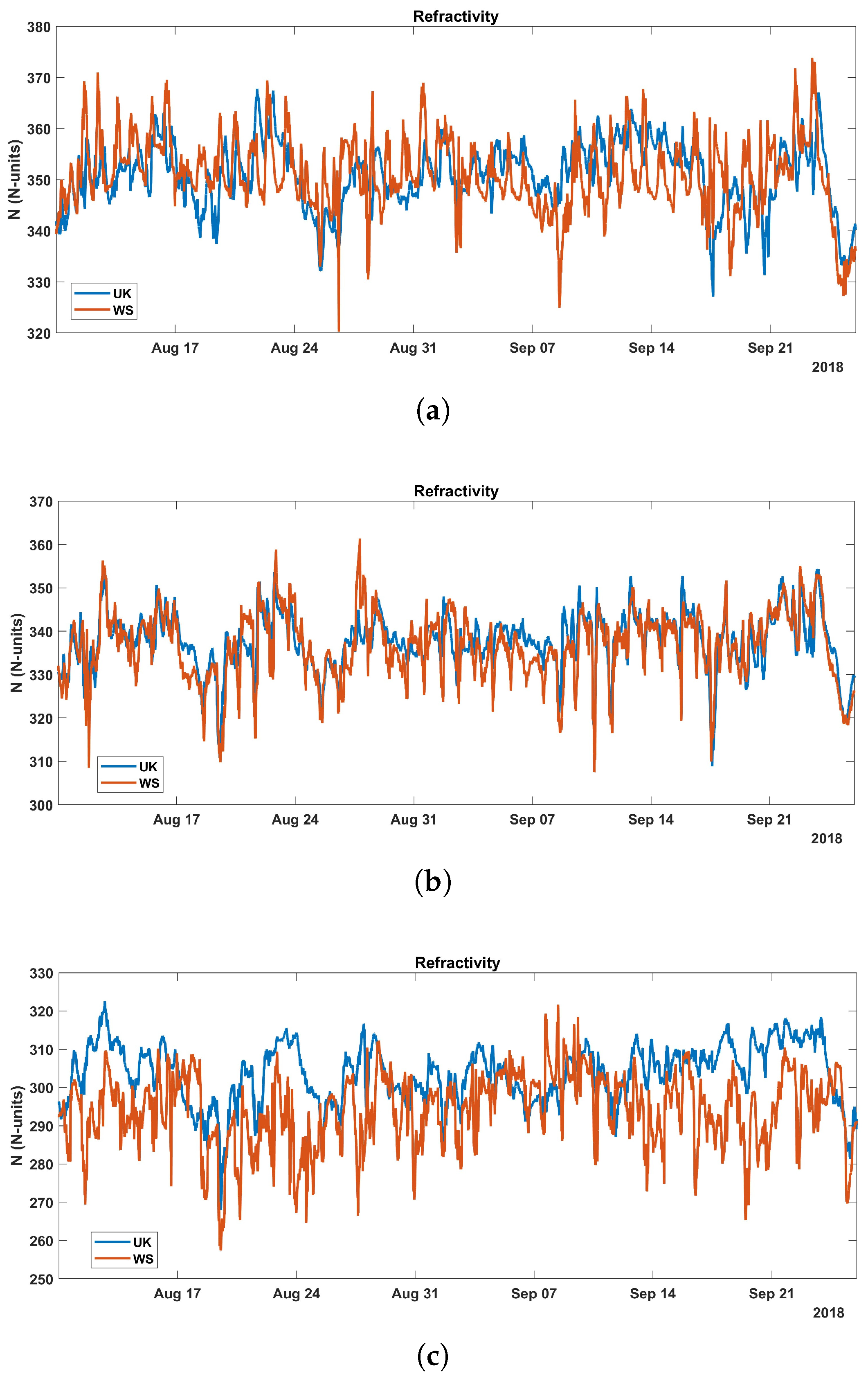
Beyond these global metrics, Figure 10 details the temporal agreement between the predicted refractivity (${\widehat{N}}_{val}$, blue line) and the observed values ($N_i$, orange line) for the three reference locations. The time series confirm that the UK model systematically reproduces the dominant altitude dependence of refractivity. Despite the inherent geostatistical challenges at higher elevations, where microclimatic anomalies naturally increase the interpolation variance, the framework maintains highly stable residual errors (achieving an overall average UK RMSE of 8.5 N-units and a MAE of 6.7 N-units) throughout the complex atmospheric cycles of the study period.

The consistently lower MAE compared to the RMSE across all stations indicates that the baseline interpolation is highly accurate, though occasionally penalized by isolated, large-magnitude residuals. These discrepancies exhibit a clear physical structure. As observed in Figure 10c and Table 1, estimation errors slightly increase at higher elevations. This characteristic pattern is driven by the intrinsic topography of the region; high-altitude areas and complex terrain naturally exhibit highly localized microclimatic variations (such as radiation inversions) that challenge macroscopic trend models. Furthermore, the lower spatial density of weather stations at higher elevations inherently increases the Kriging estimation variance in those specific altitude bands.

6. Discussion

6.1. Physical Interpretation of Interpolation Errors

An analysis of the extreme residuals, captured by the $P_{95}$ metric, reveals that these large-error episodes are heavily skewed towards specific, highly non-linear weather events. Predominantly, peak interpolation errors occur during sharp boundary-layer transitions, such as the sudden advection of coastal moisture fronts (e.g., sea breezes) or the development of tightly confined nocturnal thermal inversions in complex valleys.

To formally verify these performance gains, a paired Wilcoxon signed-rank test was applied to the absolute prediction errors of both the UK and OK models across the 6768 epochs. The test confirmed that the error reduction achieved by the UK framework is highly statistically significant ($p<0.001$) at the evaluated altitude regimes. This definitively validates that the inclusion of the deterministic vertical drift systematically and significantly resolves the severe elevation-dependent biases inherent to OK in complex topography.

From a RF operational perspective, it is critical to acknowledge that these specific, highly decoupled meteorological situations are the primary drivers of extreme anomalous wave propagation, such as localized ducting. While the UK model successfully captures the macroscopic onset of these anomalous regimes (reliably flagging regional ducting risks via the overarching vertical gradient ${\beta }_1$), the extreme spatial outliers represent sub-grid microclimatic phenomena. A shallow marine layer or a localized radiation inversion may create an intense duct that the horizontal resolution of the current 2D AWS network cannot fully resolve. Consequently, while the UK framework significantly improves regional propagation diagnostics and provides a robust, computationally stable tool for RF engineering, the distribution of its maximum residuals highlights a fundamental physical limit: the inherent difficulty of reconstructing hyper-localized atmospheric layers strictly from surface-based interpolations without supplemental 3D vertical soundings.

6.2. Propagation-Relevant Diagnostics

While reducing the interpolation error (RMSE and MAE) is a primary geostatistical objective, the ultimate operational value of the proposed UK framework lies in its direct applicability to RF propagation assessment. Atmospheric wave propagation, particularly the occurrence of anomalous phenomena such as super-refraction or ducting, is predominantly governed by the vertical refractivity gradient ($\mathrm{\Delta }N/\mathrm{\Delta }z$), rather than the absolute surface refractivity value. According to standard ITU-R definitions, standard propagation occurs near a gradient of −40 N-units/km, super-refraction falls between −157 and −79 N-units/km, and trapping (ducting) occurs when the gradient drops below −157 N-units/km [26].

A critical limitation of simpler spatial interpolation methods, such as OK, is the assumption of a stationary spatial mean. OK smooths the horizontal field but entirely obscures the vertical structural dynamics. In contrast, the proposed UK framework explicitly resolves this issue. By dynamically estimating the altitude-dependent drift ($m\left(\mathbf{x}\right)={\beta }_0+{\beta }_{1}z$) via OLS at every 10-min epoch, the algorithm inherently calculates the macroscopic vertical refractivity gradient (${\beta }_1\approx \mathrm{\Delta }N/\mathrm{\Delta }z$).

Consequently, the UK approach does not merely provide a more accurate horizontal map; its deterministic drift component serves as a direct, real-time diagnostic tool for regime classification. When the dynamically estimated ${\beta }_1$ crosses the critical ITU-R thresholds, the system can automatically flag regional ducting or super-refraction risks before the residual spatial interpolation is even completed. This demonstrates that the operational superiority of UK over OK extends far beyond modest statistical error reductions; it fundamentally recovers the physical boundary-layer gradients necessary for downstream RF decision-making and parabolic-equation modeling.

6.3. Transferability and Methodological Adaptability

Because this operational framework is demonstrated in a specific coastal–mountainous region with a relatively dense AWS network, it is necessary to explicitly discuss its transferability to other geographic domains and the boundaries of its applicability.

First, regarding network density, the stability of the automated spatial interpolation is heavily dependent on the robustness of the empirical variogram. Geostatistical best practices dictate that reliable variogram estimation requires a sufficient number of point-pairs (typically $>30$) within the shortest lag distances to accurately resolve the nugget and short-range correlation structures. In regions with significantly sparser AWS networks, the empirical variogram will become erratic. Under such degraded conditions, the automated WLS fitting procedure will likely converge toward a pure nugget model (indicating zero spatial autocorrelation). Operationally, this means the Kriging weights will become uniform, and the predictive capability of the system will gracefully degrade to rely entirely on the deterministic macroscopic drift rather than failing catastrophically.

Second, the structural advantage of the proposed UK framework is the modularity of its deterministic drift, $m\left(\mathbf{x}\right)$. In this study, elevation (z) was selected as the primary covariate because the vertical refractivity gradient strictly dominates the variance in complex terrain. However, in regions where elevation is not the primary driver such as entirely flat coastal plains or oceanic archipelagos, the atmospheric refractivity variance is typically governed by the horizontal advection of marine moisture. In such environments, the methodology can be directly adapted by substituting or augmenting the elevation variable in the drift equation with the physical distance to the coastline ($d_{coast}$). Consequently, the deterministic trend, $m\left(\mathbf{x}\right)={\beta }_0+{\beta }_1{d}_{coast}$, would systematically capture the steep boundary-layer moisture gradients transitioning from the ocean to the inland sector. This inherent mathematical flexibility ensures that the framework can be transferred to diverse global topographies, provided that the physical driver governing the local atmospheric stratification is correctly identified and integrated into the OLS drift estimation.

7. Conclusions

This work presents an applied geostatistical case study demonstrating the operational reconstruction of atmospheric refractivity fields over the highly complex topography of the Galician region. Rather than proposing a purely theoretical mathematical algorithm, this study highlights the practical, operational implementation of UK leveraging an altitude-dependent deterministic drift. By integrating a physically meaningful linear model for vertical refractivity variation with a data-driven geostatistical variogram characterization, this framework successfully captures the spatial structure of atmospheric variability in a challenging coastal–mountainous environment relying entirely on in situ measurements from a dense AWS network.

The comprehensive evaluation of the proposed methodology yielded several key operational findings:

• Vertical Stratification Modeling: A robust linear model dynamically applied at each 10 min epoch effectively estimated the macroscopic vertical refractivity gradient. Cross-validation confirmed that this drift component successfully captures the large-scale dependence of refractivity on altitude, robustly tracking diurnal cycles and synoptic meteorological shifts.
• Spatial Covariance Characterization: Residual deviations, primarily driven by local humidity fluctuations and small-scale mesoscale processes, were accurately modeled using an exponential empirical variogram. This function provided the optimal theoretical fit for the detrended spatial correlation structure across the highly variable terrain.
• High-Fidelity Regime Mapping: The integration of the vertical drift and the stochastic residuals within the UK framework produced continuous, high-resolution refractivity maps. These spatial reconstructions accurately characterize different atmospheric stability regimes, directly revealing the spatial organization of localized sub-refractive and super-refractive anomalies.

Overall, the proposed methodology provides a statistically rigorous and physically consistent operational approach for generating reliable refractivity maps from sparse surface observations, offering a computationally stable tool for real-time ducting detection and radar performance analysis.

Future work aims to evolve this 2D “time-slice” approach toward a more comprehensive multidimensional framework. First, the deterministic drift model can be refined by incorporating latitudinal, longitudinal, or coastal-distance covariates to better capture horizontal boundary-layer inhomogeneities. Second, we envisage the integration of complementary multi-sensor data sources, such as mesoscale NWP outputs, commercial microwave link attenuation data, or GNSS tropospheric tomography. Fusing these datasets would enable a more robust estimation of the atmospheric vertical profile, supporting the transition toward full three-dimensional Kriging or hybrid data assimilation models. Finally, subsequent validation efforts will expand beyond geostatistical error metrics to include direct propagation-based assessments. By executing ray-tracing simulations or radar clutter analysis over the generated UK grids, future studies will explicitly quantify the operational impact of these interpolation improvements on real-world electromagnetic system performance.