Mapping Paddy Rice Using Segmentation Techniques and Phenological Metrics Derived from Sentinel-2 Time Series in Senegal

Highlights

What are the main findings?

• Integration of image segmentation techniques and phenological metric extraction to map rice fields in the Senegal River Delta (SRD).
• A segmentation-based approach improved field boundary detection and reduced classification uncertainty compared to pixel-based methods.

What are the implications of the main findings?

• Phenological parameters such as the start, peak, and end of the growing season enabled clear discrimination between rice growth patterns.
• The combined use of temporal and spatial information enhances crop monitoring and supports sustainable rice management practices.

Abstract

Rice field mapping is essential for effective agricultural and water resource management due to high land pressure. This study aims to map paddy rice by combining segmentation techniques and phenological metrics derived from optical time series. Thus, a crop segmentation-based approach was developed using Sentinel-2 imagery (2018–2019) to assess the paddy rice extent in the Senegal River Delta (SRD). Two super-pixel segmentation algorithms were evaluated to optimize the identification of rice plots by integrating spectral and spatial characteristics from the green, red, and near-infrared (NIR) bands. In this study, the Felzenszwalb outperformed the Quickshift algorithm, achieving a median intersection over union (IoU) of 0.25 compared to 0.20 for the segmentation of rice fields. The analysis of NDVI time series enabled the identification of key stages in the rice phenological cycle. Two machine learning algorithms (i.e., Random Forest and XGBoost) were compared for rice crop detection. Random Forest delivered a better performance (AUC = 0.93, OA = 0.98, F1-score = 0.98) than the XGBoost (AUC = 0.92, OA = 0.98, F1-score = 0.98). Overall, the results indicated that the approach could accurately identify paddy rice fields, and thus improve decision making and support food security management in the region.

1. Introduction

Agriculture remains a fundamental pillar of global food security, particularly in developing countries. Among staple crops, rice holds a strategic position as a primary food source for over half of the world’s population and plays a crucial role in the livelihoods of rural populations in the Sahelian and sub-Saharan regions [1]. In the face of population growth, climate variability, and increasing pressure on natural resources, monitoring the intensification and dynamics of rice cultivation is essential to ensure sustainable and resilient production systems.

Recent advances in remote sensing have significantly enhanced large-scale crop monitoring capabilities. High-resolution time series from optical sensors (e.g., Sentinel-2, Landsat) and radar sensors (e.g., Sentinel-1) provide complementary spectral and structural information that can capture crop dynamics across seasons and diverse environments [2,3]. The emergence of cloud-based platforms such as Google Earth Engine (GEE) has further democratized access to these data and enabled the rapid development of global and regional crop mapping frameworks [4].

The study of crop phenological stages—such as emergence, growth, flowering, and maturation—has become integral to crop characterization using vegetation index time series such as NDVI, EVI, and LSWI. These indices facilitate extraction of key phenological metrics, including the start (SOS), peak (POS), and end (EOS) of the season, as well as seasonal integrals, which are critical for distinguishing crop types and growth conditions [5]. Recent work further demonstrates that integrating phenological metrics from optical and radar time series improves the robustness of temporal analysis, particularly under persistent cloud cover or in heterogeneous landscapes [6].

Despite these advances, most phenological studies have focused on large, homogeneous vegetation types or dominant crops such as maize and wheat, often overlooking the complexities of fragmented agricultural systems like those in the Senegal River Delta. These systems exhibit high intra-parcel variability due to heterogeneous hydrological conditions, diverse farming practices, and mixed cropping patterns, which complicate spectral signal interpretation and challenge traditional pixel-based classification methods [7]. Furthermore, salinity, irrigation intensity, and soil moisture variations can alter spectral responses in rice paddies, necessitating indices that account for water and soil effects [8].

To overcome these limitations, object-based image analysis (OBIA) methods have emerged as a promising alternative. By segmenting images into spatially coherent entities that correspond more closely to agricultural plots, OBIA reduces intra-class variability and enables the integration of spatial and temporal characteristics [9]. Recent research has also explored the utility of foundation models and deep learning for segmentation, such as the segment anything model (SAM) and transformer-based architectures, which demonstrate improved generalization across varied agricultural contexts compared to conventional object-based or pixel-based methods [10,11].

Accurate detection of irrigated rice in fragmented landscapes remains challenging because static spectral indices alone are often insufficient to discriminate complex crop calendars and overlapping phenological patterns. Accordingly, hybrid approaches that combine object-oriented segmentation, dense vegetation time series, and phenological characteristics have been proposed and show promising improvements in mapping performance [12,13]. Additionally, ensemble classification methods such as Random Forest and gradient boosting algorithms (e.g., XGBoost, LightGBM) have been shown to effectively handle high-dimensional, multi-source feature spaces and class imbalance, providing robust discrimination of crop types in variable environments [14].

The objective of this study is to develop an automated process for mapping rice crops using Sentinel-2 and Sentinel-1 time series in the Senegalese River Delta, which is a relevant case study due to its diversity of cropping calendars, mixed irrigation regimes, and strategic importance for regional food security. Building upon recent methodological advances in multi-sensor fusion, temporal feature extraction, and object-based classification, this work aims to provide a robust, reproducible framework that addresses key challenges posed by fragmented agricultural landscapes.

2. Materials and Methods

2.1. Study Area

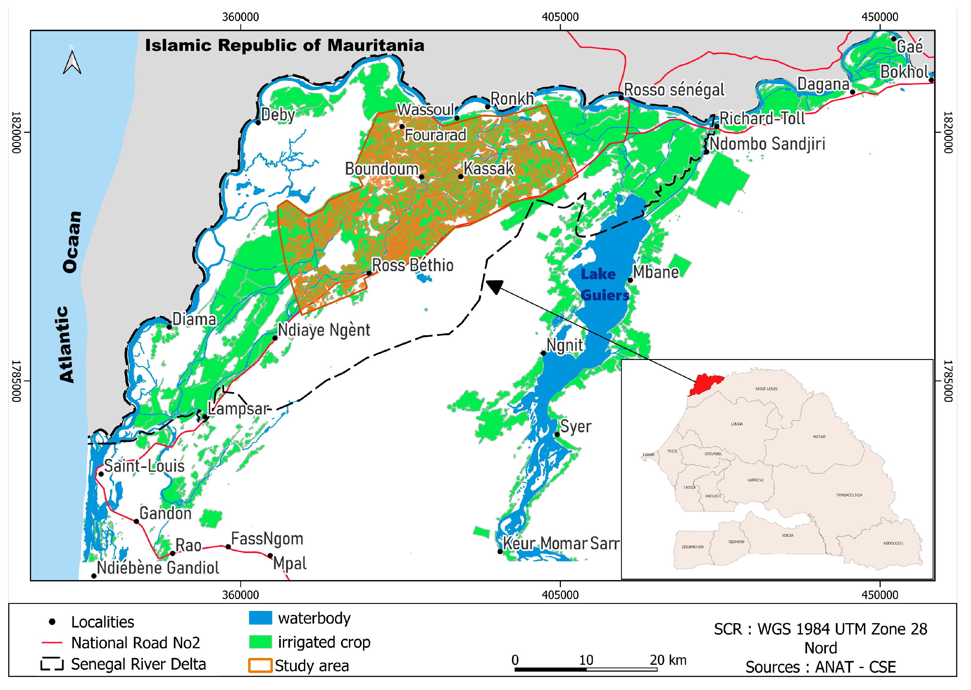
The study area is located in the center of the Senegalese River Delta (CSRD) in the extreme northwest of Senegal, more specifically within the administrative region of Saint-Louis (Figure 1). It covers an area of approximately 5000 km². The population is estimated at around 60,000 inhabitants, with a density of 13.7 inhabitants per km² [15]. The delta is bounded to the north by the Senegal River, to the west by the Atlantic Ocean, to the east by Lake Guiers, to the southwest by sand dune ridges, and to the southeast by the Ferlo Valley. The area forms a vast low-lying plain, with an average elevation not exceeding 2 m, and is subject to saltwater intrusion from the Atlantic Ocean during the dry season. It is thus a complex hydro system involving several components, including the Atlantic Ocean, watercourses, agricultural infrastructure, drainage basins, and the alluvial aquifer.

Located at the western tip of the African continent, and due to its position in the tropical zone, the SRD is exposed throughout the year to alternating airflows [16]. The climate of the SRD is characterized by a long dry season from November to May and a short wet season from June to October, governed by the north–south migration of the intertropical convergence zone (ITCZ) [17]. During the wet season, the ITCZ fully covers the study area as it moves northward, up to the edge of the Sahara. Most of the rainfall occurs between August and September [18].

The SRD receives an average annual rainfall ranging between 200 and 400 mm, concentrated over a short period of two to three months (from late July to late September), with strong interannual variability [19]. The study area lies on clay soils, which limit water infiltration and thus favor rice cultivation.

2.2. Methodology Description

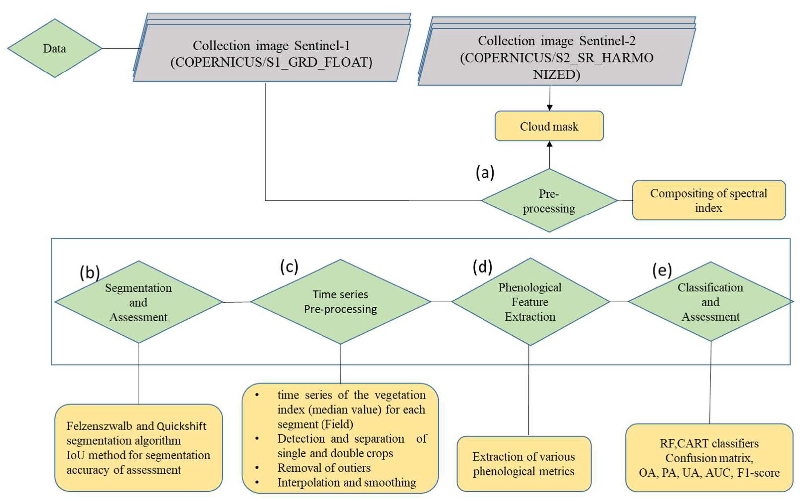
Although the overall workflow is not new, the originality of this study lies in its application and methodological refinement for highly fragmented agricultural landscapes with small field sizes (0.2–1 ha). The proposed framework explicitly addresses segmentation and classification challenges in such contexts. In addition, the study provides a critical evaluation of the contribution of SAR data, highlighting its limited impact on spatial segmentation under speckle-dominated conditions while demonstrating its added value for phenological characterization when combined with optical time series. Finally, the integration of multi-source phenological metrics and the comparison of several machine-learning models offer practical insights into model performance and data suitability for smallholder farming systems. Figure 2 shows the following main phases of this study: (a) data preprocessing, (b) image segmentation and evaluation, (c) time series analysis and (d) extraction of phenological metrics, and (e) classification and accuracy assessment.

2.3. Dataset Description and Justification

The satellite imagery consists of multitemporal Sentinel-1 SAR and Sentinel-2 optical data, accessed via the Google Earth Engine (GEE) platform (

Table 1. Description of satellite and ground data used in this study.

SAR Data
Sensor	Sentinel-1A, C band; 10 m spatial resolution
Polarization	Dual polarization: vertical transmission/horizontal and vertical receiver (VH/VV)
Orbital properties	Ascending Interferometry Wide (IW) swath mode
Year	2019
Number of images acquired	60
Optical Data
Sensor	Sentinel 2A MSI (Multispectral instrument), 10; 20; 60 m spatial resolution
Band and index	B4 (red), B3 (green), B2 (blue), B8 (near-infrared), NDVI, NDWI
Year	2019
Number of images acquired	293

). The data cover the rice-growing seasons from 2019, including the vegetative, reproductive, and maturation phases. Both optical and SAR-derived datasets provide valuable phenological information for identifying seasonal growth patterns that are specific to rice crops. Cloud contamination was addressed using the Level-2A Sentinel-2 product, allowing for the generation of cloud-free mosaics. Two key indices, which are the NDVI and VV/VH ratio, were computed for each image, and their median values were extracted. The segmentation of agricultural fields was based on seasonal composites, using the maximum NDVI (or VH/VV for radar data) to identify cultivated areas.

The optimization of segmentation algorithm parameters was performed on a 500 × 500-pixel subset (equivalent to 25 km²), with visual validation conducted in QGIS. The 500 × 500 pixel area was selected because it represents a heterogeneous portion of the landscape, including rice fields, other crops, and irrigation features. This size provides a balance between spatial representativeness and computational efficiency, allowing for reliable calibration of segmentation parameters while remaining tractable for iterative testing. The optimized parameters were then applied to the full study area to assess their robustness. This validation involved comparing the segmentation results to the manually delineated field boundaries provided by the study area Development and Management Authority (SAED) in shapefile format. Then, the algorithm was applied to the entire irrigation scheme, resulting in a vector file representing the segmented field boundaries. To eliminate irrelevant objects such as uncultivated land, roads, and drainage channels, a minimum area threshold of 80,000 m² (8 ha) was applied. The 8-ha threshold was introduced to reduce the influence of highly fragmented and poorly segmented parcels, which are more prone to mixed pixels and segmentation errors. This choice does not aim to systematically exclude small rice fields but to ensure a more reliable evaluation of the proposed methodology. Nevertheless, we acknowledge that this threshold may bias the accuracy estimates toward better-performing parcels. This filtering step enhanced the accuracy of the segmentation by reducing noise and excluding artifacts from the final output.

For the classification, the Random Forest (RF) [20] and XGBoost [21] models were tested on a dataset obtained from the Quickshift and Felzenszwalb segmentation algorithm, with 1017 samples used for training and 438 samples for validation, split into 70% for training and 30% for testing. The influence of phenological features was assessed using Scikit-learn version 1.4.2 by measuring the impact of randomizing each variable on the model’s accuracy. The number of samples per crop class was used for the classification experiments conducted in this study on the entire validation dataset. These irrigated crop samples include irrigated rice (120 polygons), irrigated mixed crops (121 polygons) and irrigated vegetables (111 polygons). The spatial distribution and environmental coverage of the samples, including differences in irrigation conditions, soil types, and crop characteristics, to address potential limitations in model generalization for saline–alkali paddy fields and marginal irrigation areas. These polygons originate from the SAED data, which were collected in the season 2018–2019. These reference polygons were used to train and validate the classification of irrigation.

The analysis is based on a single season, 2018–2019, due to the lack of reliable validation data for other years. Consequently, the conclusions have been revised and more cautiously formulated to avoid claims of long-term applicability. The proposed approach is now presented as a methodological framework with potential for multi-year monitoring, subject to the availability of appropriate multi-year validation data.

2.4. Segmentation Process

2.4.1. Compositing of Spectral Index

Two image segmentation algorithms were tested: Felzenszwalb [22] and Quickshift [23]. The five different input combinations (spectral bands and vegetation indices) used for the segmentation are as follows:

Composite 1: CIR image composed of the bands NIR (B8), Rouge (B4), and Blue (B3);

Composite 2: Radar image including the vertical (VV) and horizontal (VH) polarizations, along with their ratio (VH/VV);

Composite 3: Image representing the maximum values of the Normalized Difference Vegetation Index (NDVI);

Composite 4: Image showing the maximum values of the VH/VV polarization ratio;

Composite 5: Composite image combining three vegetation indices: NDWI (Normalized Difference Water Index) $NDWI=\left(Nir-Swir\right)/\left(Nir+Swir\right)$, NDVI (Normalized Difference Vegetation Index) $NDVI=\left(Nir-Red\right)/\left(Nir+Red\right)$ and RVI (Radar Vegetation Index), with RVI calculated as follows:

$$RVI={\displaystyle \frac{4VH}{VH+VV}}$$

(1)

These various composite images, derived from both Sentinel-1 (SAR) and Sentinel-2 (optical) data, were employed to evaluate which segmentation algorithm produced the most accurate delineation of agricultural fields. The objective was to identify the best-performing input for superpixel-based segmentation, enabling accurate delineation of rice plots and providing a robust foundation for subsequent crop classification [24].

2.4.2. Validation of the Segmentation Process

The validation of the segmented objects was performed using the Intersection over Union (IoU) [25] metric (Equation (1)), which is widely used to assess the segmentation quality by comparing the algorithm-generated polygons to ground-truth reference polygons (SAED data). The overlay method from the GeoPandas library was utilized to compute the IoU values, enabling efficient implementation within a geospatial data processing environment.

$$IoU=\left|{\displaystyle \frac{A\cap B}{A\cup B}}\right|={\displaystyle \frac{{Area}_I}{{Area}_U}}={\displaystyle \frac{TP}{FN+TP+FP}}$$

(2)

TP: true positives; FP: false positives; TN: true negatives; and FN: false positives.

The resulting segments were then used as a basis for crop classification. Temporal indicators, such as the seasonal evolution of vegetation indices and radar backscatter signals, were extracted. These features were used as input in a supervised classification model to differentiate between various crop types.

2.5. Computation of Phenological Metrics

In the first step, we used the 293 available images to construct the NDVI time series for the 2019 dry season, derived from the Sentinel-2 product, as specified in the document. These time series allow monitoring of the seasonal dynamics of vegetation and biomass [26]. When relevant, radar data (Sentinel-1) were integrated to extract backscatter parameters (VV/VH ratio), which are sensitive to the structural and hydrological properties of crops [27].

In the second step, the raw time series were preprocessed to correct noise, temporal gaps, and outliers. Unreliable observations were filtered, and missing data were interpolated. Smoothing was applied to reduce non-representative fluctuations while preserving the true seasonal dynamics. The Savitzky–Golay filter was used with a window of 5–7 observations and a polynomial degree of 2 [28]. For single-season series, more advanced methods such as Gaussian smoothing or the double logistic function were applied with a 60-day moving average (MA) and an NDVI threshold of 0.4 to identify phenological transitions [29]. In the third step, to facilitate correspondence with field observations and reduce intra-field variability, vegetation index values were averaged over a 3 × 3 pixel window.

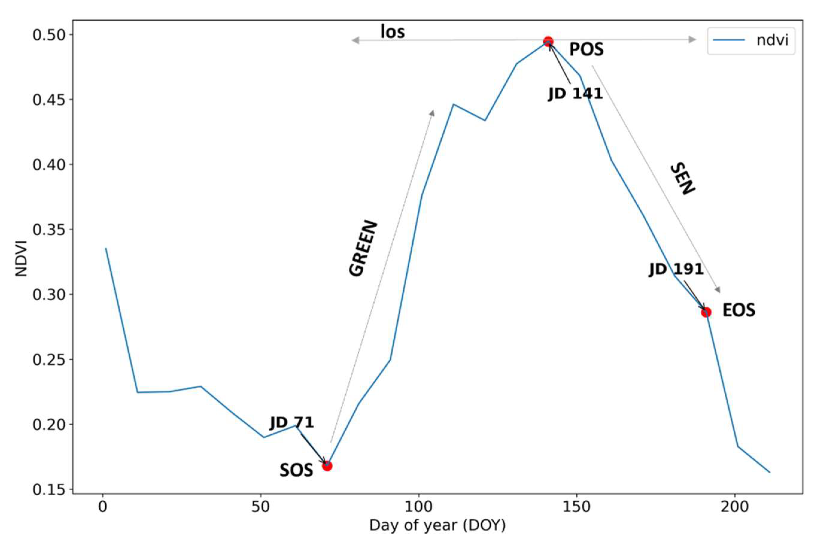
In the fourth step, phenological stage estimation was based on the analysis of NDVI (and radar backscatter) time series. The NDVI time series was used as input for the feature extraction process (Figure 3). The main phenological metrics were extracted: the start of the season (SoS) was identified when the index exceeded the relative threshold, the peak of the season (PoS) corresponded to the maximum index value, and the end of the season (EoS) was detected when the index fell below the threshold. The season length, as well as complementary metrics such as the maximum NDVI value and its date, as well as the greening and senescence periods, were calculated to characterize vegetation dynamics [30]. Extracted phenological metrics were validated against field observations and historical crop calendars, with SOS and EOS estimates being accurate within ±7 days of actual planting and harvesting dates. The entire pipeline is automated and reproducible, with preprocessing in GEE and analysis in Python version 3.9.19, ensuring consistent extraction of phenological metrics across all parcels.

This approach, calibrated with field observations, achieved an accuracy of approximately 10 days in locations with less than 10% missing data. The SOS and EOS dates were defined, respectively, at 20% and 50% of the seasonal NDVI amplitude. The smoothed curves were fitted to the upper envelope of the NDVI values to extract nine phenological metrics (see Figure 3).

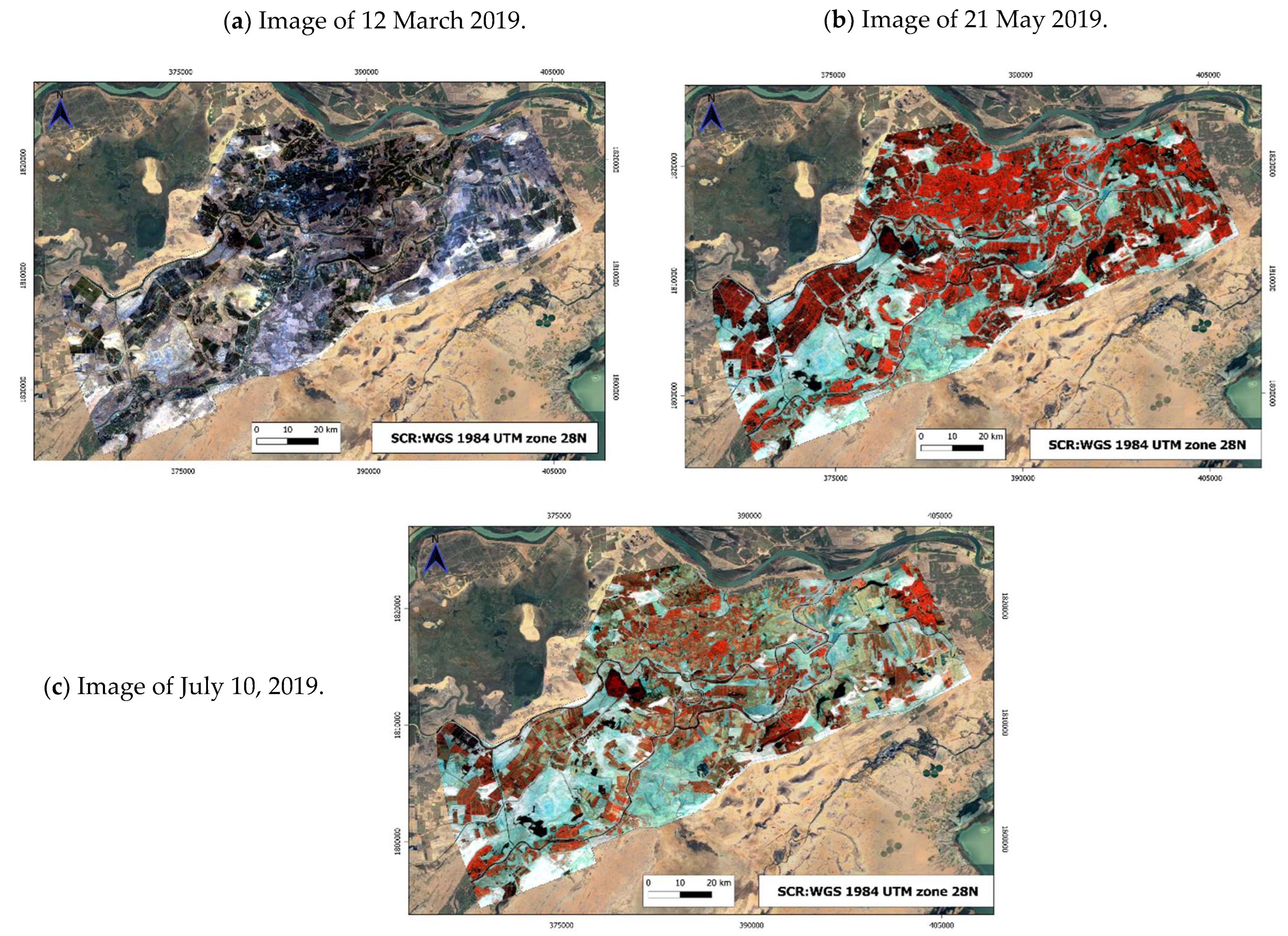
When both optical and radar data were available, a multi-sensor fusion was performed to improve temporal continuity and the robustness of phenological metrics (

Table 2. Phenological metrics derived from NDVI time series.

N°	Variable	Abbreviation	Definition
1	Start of season	sos_d	Date at which the left boundary reaches 20% of the amplitude.
2	End of season	eos_d	Date at which the right boundary decreased to 50% of the amplitude.
3	Peak season	pos_d	Date of the seasonal peak value.
4	Season length	los	Date within the period from SOS to EOS.
5	Start of season value	sos_v	The initial positive slope on the green (increasing vegetation) side of the curve.
6	End of season value	eos_v	The final negative slope on the senescent (declining vegetation) side of the curve.
7	Peak season value	pos_v	The highest NDVI value of the season.
8	Large integral	Green (Greening)	Rate of NDVI increase at the start of the season (SOS), between 20% and 80% of the amplitude on the left side.
9	Small integral	Sen (senescence)	Rate of NDVI decrease at the end of the season (EOS), between 20% and 80% of the amplitude on the right side.

), combining the spectral sensitivity of optical data with the structural and hydrological information provided by radar, independent of atmospheric conditions(Figure 4) [31].

Finally, the extracted phenological metrics were aggregated at the field scale to reduce intra-field variability and facilitate their use for crop classification or agricultural productivity assessment. Integrating these metrics into machine learning and deep learning models improves mapping and crop monitoring performance [32].

Thus, this methodology combines rigorous preprocessing, optimized smoothing with moving averages and NDVI thresholds, spatial adjustment for field correspondence, and multi-sensor fusion, providing a robust, reproducible approach that is suitable for analyzing seasonal crop dynamics.

2.6. Evaluation of Classifier Performance

Several indicators, including overall accuracy (OA), precision (P), recall (R) [33], F1-score, and the area under the curve (AUC) [34] of the receiver operating characteristic (ROC) curve, were used for the evaluation.

Overall accuracy (OA): The ratio of the number of correctly predicted observations to the total number of observations.

$$OverallAccuacy={\displaystyle \frac{TP+TN}{TP+TN+FP+FN}}$$

(3)

Producer’s accuracy (PA): Measures the proportion of the positive instances that are correctly identified among all instances identified as positive by the model.

$$Precision={\displaystyle \frac{TP}{TP+FP}}$$

(4)

User’s accuracy (UA): Measures the proportion of correctly identified positive instances among all the truly positive instances in the data.

$$Recall={\displaystyle \frac{TP}{TP+FN}}$$

(5)

Harmonic mean of precision and recall.

$$F1score={\displaystyle \frac{2\times Precision\times \mathrm{R}\mathrm{e}\mathrm{c}\mathrm{a}\mathrm{l}\mathrm{l}}{Precision+Recall}}$$

(6)

One of the main challenges in classification evaluation lies in the class imbalance, which can introduce bias into the results. Indeed, OA may vary depending on the distribution of samples in the confusion matrix, even if the classification performance remains constant [35]. To overcome this bias, methods such as the area under the ROC curve (AUC-ROC) were used. These were adapted to the imbalanced multiclass classification by producing a ROC curve for each pair of classes. The comparison between Random Forest (RF) and XGBoost is motivated by their widespread use and proven performance in rice mapping. RF, based on bagging, is robust to noise, handles correlated features well, and performs reliably with limited training samples, making it suitable for multi-source time-series data [36]. XGBoost uses sequential boosting to model complex non-linear relationships and feature interactions, with regularization to reduce overfitting, which is particularly useful for phenology-based rice classification using optical and SAR data [37]. Comparing these two complementary ensemble methods provides a robust assessment of classification performance in rice mapping.

3. Results

3.1. Analysis of the Parameters of the Segmentation Algorithms

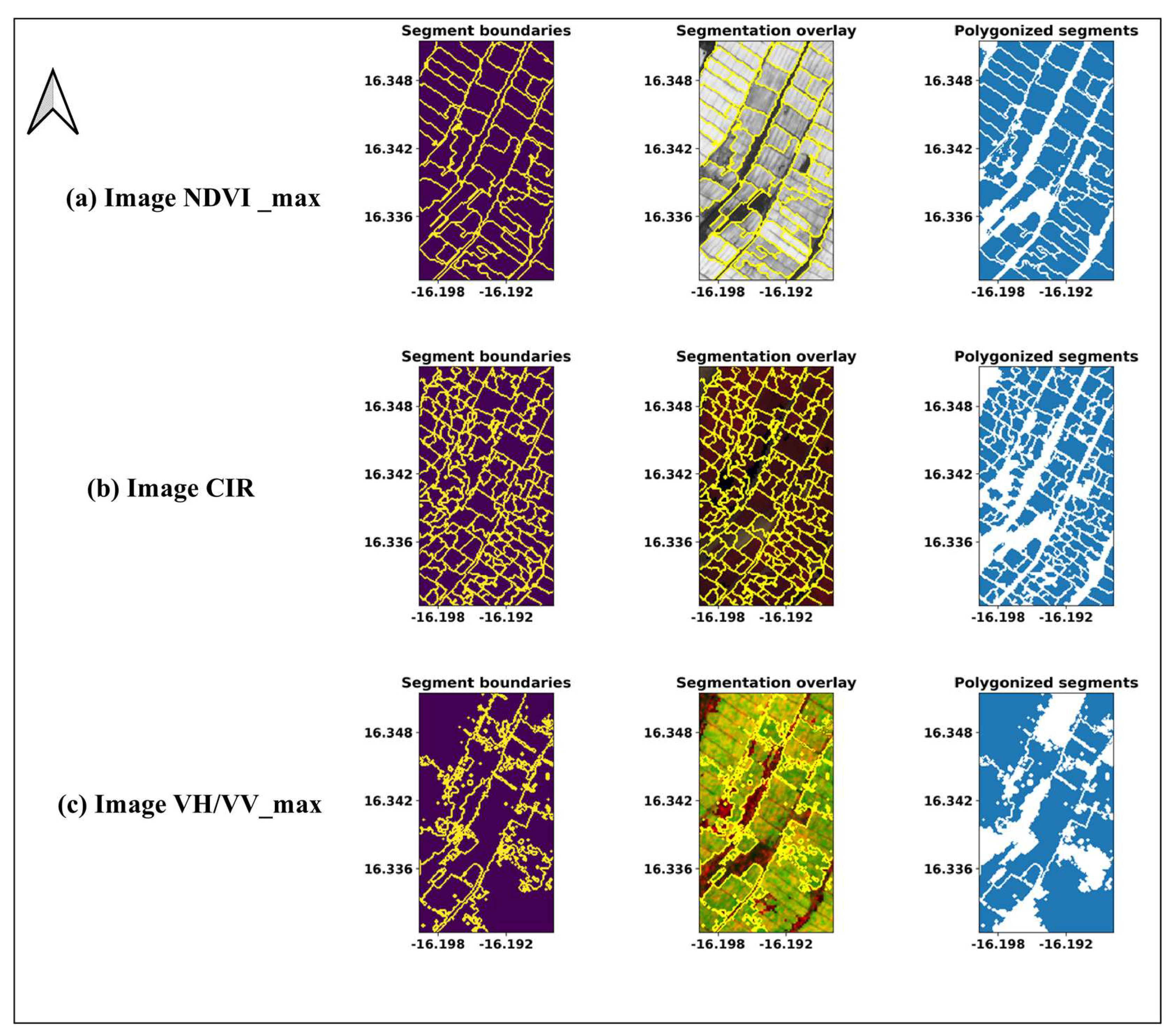
The Felzenszwalb algorithm, applied to a maximum NDVI image and a maximum VH/VV image, uses several parameters to optimize segmentation. Sigma (σ) controls the smoothing of the NDVI image to reduce noise while preserving vegetation boundaries. Min_size defines the minimum size of a segment; small vegetation regions are merged with neighboring ones if they are too small. Scale adjusts the algorithm’s sensitivity to differences in NDVI values between segments, influencing the segmentation granularity. The results obtained with the Felzenszwalb algorithm indicate that although the generated segments are large and homogeneous (Figure 5a,b, in blue), their precision can sometimes be insufficient. On both optical (NDVI_max) and radar images (VH/VV_max), a merging of distinct objects is observed. This phenomenon is due to the excessive size of the segments, which is particularly noticeable in Figure 5b, resulting in under-segmentation and blurred boundaries between certain objects. Such segmentation is less suitable for heterogeneous agricultural environments, as also noted by [38]. The best performance was obtained with a scale of 100, sigma of one, and a min_size parameter between 1850 and 2175, which helped reduce over-segmentation and better delineate fields. It should be noted that min_size values that are too large or too small degrade accuracy.

The Quickshift algorithm was tested with different parameters (ratio, kernel_size, max_dist) on a CIR image (Figure 5b) composite 1 (composite 2, composite 5 where not presented) to refine segmentation. The sigma parameter controls the scale of the local density approximation, while max_dist determines the level of hierarchical segmentation. The ratio parameter adjusts the trade-off between distance in color space and image space; however, its impact is less significant than the other parameters. Therefore, selecting the appropriate Quickshift algorithm parameters is essential to achieve optimal segmentation tailored to the specificities of the processed data. In contrast, the Quickshift algorithm, which relies on hierarchical mode-based segmentation, produced finer and more accurate segments, as shown by the blue result in Figure 5c. This method is better suited to agricultural environments due to the flexibility of its parameters and its ability to capture the complex details of fields, as demonstrated by [39]. In conclusion, the kernel_size parameter plays a crucial role in distributing segment variability, according to the spectral and spatial characteristics of the images.

3.2. Comparison of the Segmentation Algorithms

The comparison between the Felzenszwalb and Quickshift algorithms highlights notable differences in segmentation accuracy and computational efficiency.

Table 3. Intersection over union (IoU) results for five input combinations across both segmentation algorithms.

Composites	Bands/Index	IoU	Tested Algorithms
Composite 1 *	B8, B11, B12	0.20	Quickshift
Composite 2	VV, VH, VH/VV	0.04	Quickshift
Composite 3	Ndvi_max	0.25	Felzenszwalb
Composite 4	VH/VV_max	0.05	Felzenszwalb
Composite 5	Ndvi, ndwi, rvi	0.03	Quickshift

presents the test results conducted on optical images and radar images, as well as on a combination of both, using the two segmentation algorithms. The objective of this analysis is to identify the sensor, or combination of sensors, that provides the best utility value for crop mapping within the scope of this study.

The Felzenszwalb algorithm generates a median IoU of 0.25 when applied to the optical image (NDVI_max), compared to only 0.05 for the radar image (VH/VV_max).

The Quickshift algorithm, although producing an IoU of 0.2 for the spectral composition derived from the CIR image, requires a longer processing time of about eight minutes for the whole scheme. This performance remains superior to that obtained with the combination of optical and radar indices (NDVI, NDWI, RVI), which displays an IoU of only 0.03. Nevertheless, even with this improved result, Quickshift’s performance remains lower than that of Felzenszwalb.

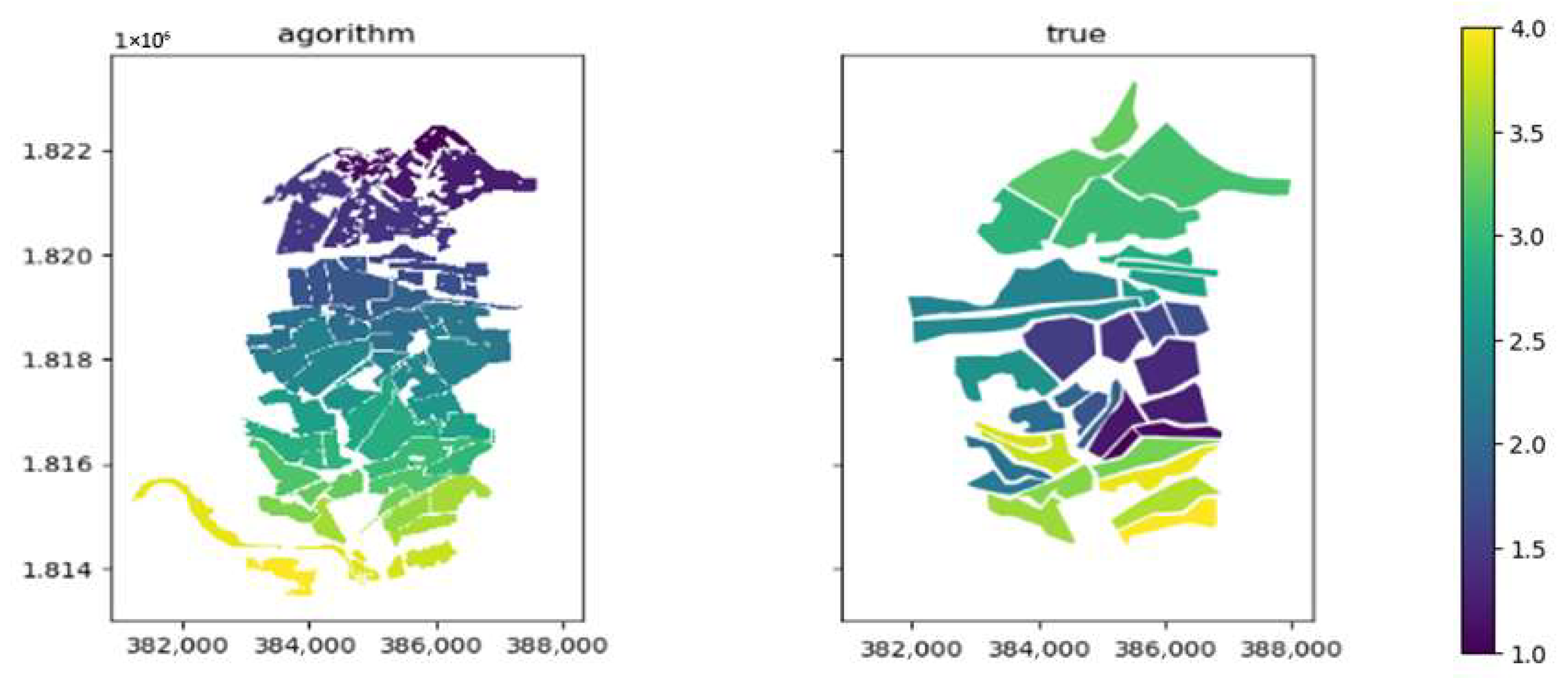
Thus, after this evaluation, we observed two types of segmentation errors when comparing the algorithm’s results with the reference polygons in Figure 6. Over-segmentation, at a relatively small scale, is mainly due to a lack of contrast between pixels, leading to fragmented fields. Under-segmentation, at a larger scale, results in the merging of distinct plots into a single segment, thereby compromising detection accuracy.

The performance of each method strongly depends on the type of data used, as well as on the selected parameters. In the context of this study, the contribution of radar data to improving the spatial segmentation quality appears limited, mainly due to the presence of speckle noise, which degrades the readability of structures and field boundaries [40]. This limitation is further amplified by the strong fragmentation of agricultural fields in the study area, characterized by relatively small parcel sizes ranging from 0.2 to 1 hectare. Small field sizes, combined with high spatial heterogeneity, make image segmentation particularly challenging, regardless of the sensor used, and complicate the assessment of the reliability of segmentation accuracy [41,42]. By contrast, agricultural contexts with larger and more spatially homogeneous fields generally lead to improved segmentation and classification performance, owing to clearer boundaries and stronger intra-parcel consistency [43,44]. Nevertheless, radar data remain highly valuable for the structural and temporal characterization of surfaces, particularly for phenological analysis and crop monitoring, especially when combined with optical data through multi-sensor fusion approaches [45,46].

3.3. Phenological Metrics Analysis

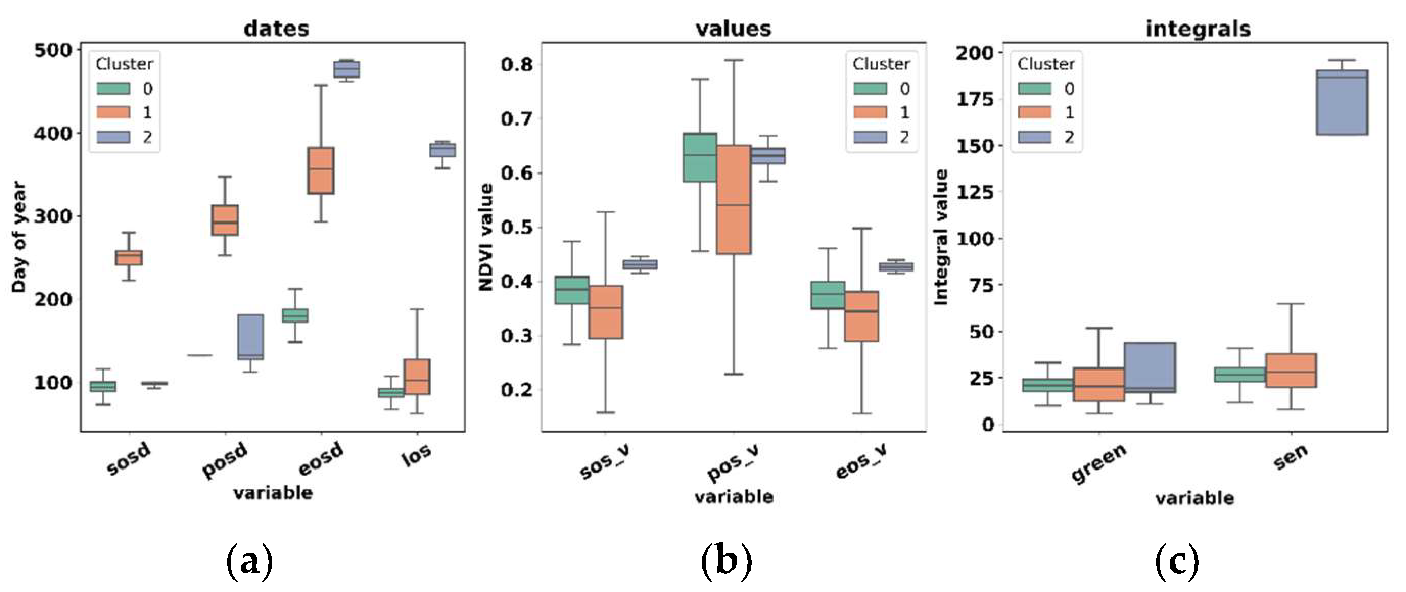
The approach combining phenological metrics and unsupervised classification allowed for the identification of different agricultural seasons, based on vegetation indices extracted from satellite image time series. Nine phenological metrics (sos_d, eos_d, pos_d, los, sos_v, eos_v, pos_v, green corresponding to the greening phase and sen to the senescence phase), presented in Table 3, were selected as input variables. These parameters include key dates and values characterizing the rice crop cycle, notably the start, peak and end of the season, as well as phases of growth and decline in green biomass. The data were normalized before being submitted to the Mean Shift algorithm, which grouped the plots into three distinct classes corresponding to the main identified cropping seasons.

The graphical representations in Figure 7 show boxplots for three types of parameters—dates, values and integrals—calculated from the nine phenological metrics, highlighting statistical trends within each identified class.

The results indicated that NDVI values and integrals exhibit similar profiles across the cluster, suggesting an overall homogeneous vegetative development from one season to another. In contrast, phenological dates, notably the vegetation peak date (pos_d), clearly differentiated the three identified groups. This variable emerged as a particularly relevant temporal marker, revealing a significant spread of flowering dates, starting from Julian day 300. This temporal shift underscores the diversity of agricultural calendars in the study region. Moreover, the greening and senescence integrals presented relatively low values, reflecting limited biomass accumulation during these transitional phases of the crop cycle.

3.4. Importance of Input Variables in the Classification Process

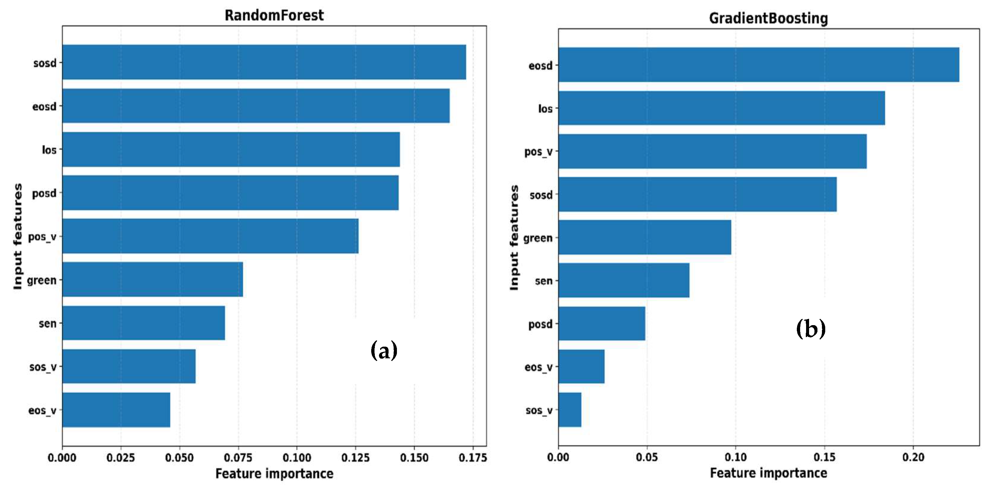
Figure 8 presents the ranking of input variables according to their relative importance in the Random Forest and Gradient Boosting models. The analyzed variables are divided into phenological temporal indicators (dates and season length) and value-based indicators related to growth intensity and spectral components.

Overall, both models highlight the predominance of phenological temporal variables over value-based variables. Key dates of the crop cycle, as well as the length of the growing season, constitute the main explanatory factors of the studied phenomenon.

For the Random Forest model, sosd and eosd exhibit that the highest importance values exceed 15%, reflecting the strong influence of the start and end dates of the growing season. These variables are followed by los and posd, whose contributions remain comparable at about 14%, indicating that season length and peak timing also play a significant role. Value-based variables, particularly pos_v, still show a non-negligible contribution, while green, sen, sos_v, and eos_v display lower importance levels (about 5%). This relatively balanced distribution suggests that the Random Forest model integrates multiple dimensions of the available information.

In contrast, the Gradient Boosting model shows a more pronounced concentration of importance on a limited number of variables. The eosd variable clearly dominates, exceeding 20%, followed by los, emphasizing the predominant role of the end of the season and the duration of the crop cycle. The variables pos_v and sosd occupy intermediate positions reaches approximately 15%, whereas the value-based variables sos_v and eos_v become marginal around zero. This structure reflects the more selective nature of the gradient boosting approach, which progressively reinforces the influence of the most contributive variables.

The comparison between the two models indicates that, although both agree on the central importance of phenological temporal indicators, their weighting strategies differ. The Random Forest model distributes importance across a broader set of variables, whereas the gradient boosting model focuses on the most discriminative ones.

3.5. Accuracy Assessment of Algorithms for Classification

Table 4. Classification results of the different proposed models.

Label	N° Sample		Precision		Recall		F1_Score		AUC
			XGB	RF	XGB	RF	XGB	RF	XGB	RF
Irrigated mixed crop	121		0.33	0.50	0.17	0.17	0.22	0.28	0.86	0.85
Irrigated rice	120		0.98	0.98	0.99	0.99	0.98	0.99	0.92	0.93
Irrigated vegetables	111		0.67	0.71	0.80	1	0.73	0.83	1	1
Macro average			0.66	0.73	0.65	0.72	0.64	0.69
Weighted average			0.96	0.97	0.96	0.97	0.96	0.97	0.93	0.93

presents the classification performance of the XGBoost (XGB) and Random Forest (RF) models for three irrigated crop classes, using precision, recall, F1-score, and AUC as evaluation metrics. These performance measures are widely used in remote sensing and machine learning to assess classification quality [47].

For the irrigated rice class, both models show excellent and consistent performance. Precision, recall, and F1-score values are close to 1.0 for both XGB and RF, indicating high classification reliability. The AUC values (0.92 for XGB and 0.93 for RF) further confirm the strong separability of this class in the feature space. This suggests that irrigated rice exhibits a clear phenological and spectral signature, facilitating discrimination by both models.

The irrigated vegetables class also demonstrates strong performance, with RF slightly outperforming XGB. RF achieves perfect recall (1.00) and a higher F1-score (0.83) compared to XGB (0.73). The AUC values reaching 1.00 for both models indicate excellent class separability. These results align with previous findings, where ensemble learners such as Random Forest and gradient boosting frameworks excel in handling non-linear class boundaries [48].

In contrast, the irrigated mixed crop class shows significantly lower performance for both models. Precision and recall values are low, particularly for recall (0.17), resulting in weak F1-scores. This indicates class confusion with other irrigated crop categories. The reduced performance can be attributed to the intrinsic heterogeneity of mixed cropping systems, which tend to exhibit overlapping phenological and spectral characteristics. Despite this, relatively high AUC values (0.85–0.86) suggest that the models retain a moderate ability to distinguish this class at a probabilistic level.

The macro-average metrics highlight clear differences between the two models. Random Forest consistently outperforms XGBoost, showing higher macro precision (0.73 vs. 0.66), macro recall (0.72 vs. 0.65), and macro F1-score (0.69 vs. 0.64). This indicates that RF provides a more balanced performance across classes, including the more difficult ones.

The weighted-average results show very high and similar values for both models (around 0.96–0.97 for precision, recall, and F1-score). These high scores are largely influenced by the dominant class with strong performance, particularly irrigated rice. The weighted AUC is identical for both models (0.93), confirming their overall robustness [49].

Overall, both models demonstrate strong classification capabilities for homogeneous irrigated crops, especially irrigated rice. However, Random Forest shows a slight advantage in terms of balanced performance across classes, particularly for irrigated vegetables and according to macro-average metrics. The lower performance for irrigated mixed crops highlights the challenge of classifying heterogeneous land-use categories and suggests that enhanced feature engineering or hierarchical classification strategies might be necessary to improve discrimination.

These results support the use of Random Forest as a robust baseline model, while also highlighting the complementary strengths of XGBoost, particularly in well-defined crop classes [50].

Classification with RF

The analysis of the confusion matrix in

Table 5. Confusion matrix and validation results of the NDVI time series with the XGB classifier.

Predicted
Actual		Irrigated Mixed Crops	Irrigated Rice	Irrigated Vegetables	Total of Classified Sample	Producer’s Accuracy (%)
	Irrigated mixed crops	1	4	1	6	16
	Irrigated rice	1	230	1	232	99
	Irrigated vegetables	0	0	5	5	100
	Total of reference samples	2	234	7	243
	User’s accuracy (%)	50	98	71		OA = 97%

reveals an excellent overall performance of the classification model, with an overall accuracy (OA) of 97%. However, significant differences are observed among the classes. The irrigated rice class shows very high producer’s (99%) and user’s (98%) accuracies, indicating that most rice plots were correctly identified and predicted with high reliability. In contrast, the irrigated mixed crops class records a low producer’s accuracy (16%) and user’s accuracy (50%), reflecting a strong confusion with irrigated rice fields. This poor performance may be explained by the spectral similarity between the two crop types and by the limited representation of mixed crops in the training dataset. The irrigated vegetables class achieves a perfect producer’s accuracy (100%) but a more moderate user’s accuracy (71%), suggesting some misclassifications. Overall, these results highlight the robustness of the model in detecting irrigated rice, while emphasizing the need for a more balanced sampling strategy and improved class representation to enhance the discrimination of minority crop types.

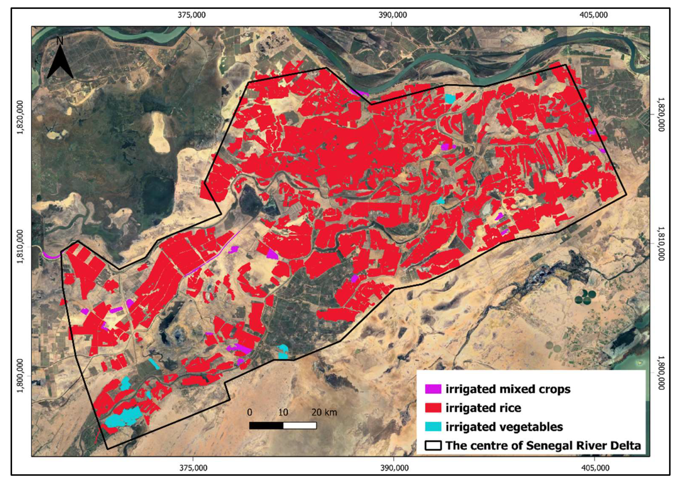
Figure 9 analyses the classification results obtained using the Random Forest (RF) algorithm, based on optical data (NDVI). Overall, the “irrigated rice” class, shown in red, is clearly identified with the well-defined boundaries of the rice fields. Other land cover classes, such as irrigated mixed crops and irrigated vegetables, are also well-distinguished, displaying clearly structured textures. These results demonstrated the model’s ability to effectively differentiate the various spectral signatures associated with different crop type classes.

The results were generally satisfactory, especially in homogeneous areas. However, some agricultural plots exhibited intra-field heterogeneity, with segments classified into different categories, indicating either spectral variability within the field or limitations of the model in generalizing effectively in complex contexts. Furthermore, certain specific crops, which are less prevalent or cultivated atypically in the study area, were not correctly identified, resulting in reduced accuracy for their detection on the classified map.

4. Discussion

The overall methodology combined segmentation, spectral–temporal analysis and classification to improve the mapping and characterization of irrigated crops. Each step played a complementary role in enhancing the accuracy and interpretability of the results.

The segmentation process was a crucial step for delineating homogeneous agricultural units and reducing spectral variability within fields. This object-based approach allowed for better correspondence between satellite observations and actual agricultural parcels compared to pixel-based methods [51]. However, segmentation accuracy depended on the spatial resolution of the images and the selection of appropriate segmentation parameters, which could affect boundary precision and the detection of small fields [52]. Although Felzenszwalb tends to over-segment, it effectively captures parcels that are smaller than one hectare, which are typical of fragmented agricultural landscapes, whereas Quickshift often overlooks these micro-plots. Nevertheless, overall segmentation accuracy remains below the thresholds commonly reported in the literature (IoU > 0.4), primarily due to spatial heterogeneity and small parcel sizes. This finding aligns with previous studies [53], which emphasize the importance of balancing spatial homogeneity and spectral similarity when selecting segmentation parameters. The extreme fragmentation of parcels in the delta therefore represents a major limiting factor for precise object delineation.

Spectral and phenological analyses provided essential information for understanding crop dynamics over time [54]. Temporal metrics derived from vegetation indices enabled the differentiation of crop types, based on their growth patterns and seasonal behavior [55]. These metrics reduced confusion between classes with similar spectral responses during certain periods, such as between irrigated rice and mixed crops. Nevertheless, the accuracy of this step was influenced by data availability, cloud cover and the temporal resolution of the imagery. The superiority of temporal variables over intensity values for characterizing agricultural seasons was confirmed, demonstrating that a detailed analysis of key phenological dates is essential for understanding crop dynamics in fragmented agricultural environments [56].

Regarding classification performance, both the Random Forest (RF) and XGBoost (XGB) algorithms achieved high overall accuracy and AUC values, confirming their strong capability to discriminate irrigated crop classes. However, RF slightly outperformed XGB in terms of balanced performance across classes, as reflected by higher macro-average precision, recall, and F1-score values.

The superior performance of RF is particularly evident for the irrigated vegetables class, where it achieved perfect recall and a higher F1-score compared to XGB. This behavior highlights the robustness of RF when dealing with class variability and non-linear relationships, as well as its ability to maintain stable performance across different crop types. These results are consistent with previous studies reporting the resilience of RF to noise, data heterogeneity, and overfitting in remote sensing classification tasks [57,58].

In contrast, XGBoost demonstrated excellent performance for well-defined and homogeneous classes, especially irrigated rice, with precision, recall, and F1-score values close to unity. This confirms the strong discriminative power of XGB when class signatures are clearly separable. Nevertheless, XGB showed comparatively lower performance for more heterogeneous classes, particularly irrigated mixed crops, where both precision and recall remained low. This suggests a higher sensitivity of XGB to class imbalance and intra-class variability.

Despite the reduced class-wise performance for irrigated mixed crops, both models exhibited relatively high AUC values for this class, indicating that they retain a reasonable probabilistic discrimination capacity. The low recall values, however, reveal persistent confusion with other irrigated crop classes, which is likely due to overlapping phenological and spectral characteristics that are inherent to mixed cropping systems.

Overall, these results suggest that while XGBoost is highly effective for dominant and phenologically consistent crop classes, Random Forest provides a more stable and balanced classification across all classes. The observed limitations for heterogeneous and minority classes emphasize the need for more balanced training datasets and the potential integration of additional features, such as texture metrics or multi-temporal indices, to improve class separability.

Furthermore, the study emphasizes the limitations of relying solely on OA in the presence of imbalanced data, where metrics such as AUC provide a more reliable evaluation of model performance, especially for underrepresented classes in the sample.

Overall, the integration of segmentation, phenological metrics and advanced classification techniques proved effective in improving crop mapping accuracy in highly fragmented irrigated landscapes. Despite the challenges associated with parcel heterogeneity and class imbalance, the results achieved here compare favorably with those reported in similar studies [59], confirming the robustness and relevance of the proposed methodological framework.

The analysis highlighted systematic confusion between several classes and irrigated rice, suggesting that NDVI spectral signatures alone are not sufficiently discriminative. To improve classification, it is recommended to incorporate additional explanatory variables such as humidity indices and other vegetation indices, and to refine the observation periods used in the time series.

5. Conclusions

This work highlights the relevance of a hybrid approach (segmentation combined with supervised classification) for characterizing cropping cycles in the context of fragmented plots. It also illustrates methodological challenges related to parcel size, spectral confusion and the choice of evaluation metrics, while providing directions for future research on large-scale agricultural image segmentation, particularly in regions like the Sahel.

The results demonstrate the importance of precise segmentation of rice plots and the exploitation of phenological features. The use of appropriate indicators (AUC, OA) enabled a rigorous evaluation of models, improving crop discrimination. Future perspectives of this research include the integration of advanced segmentation methods (deep learning), the use of metrics better suited for imbalanced datasets and the incorporation of auxiliary data (climatic factors) to enhance prediction accuracy.

Finally, this study emphasizes the importance of an integrative approach, combining multiple data sources and advanced methods for a better understanding of cropping cycles and sustainable management of agricultural resources. Such an approach would be valuable for establishing an inventory and monitoring system for paddy rice, facilitating decision-making and policy implementation to benefit smallholder farmers in the delta region.

References

1. Jiang, J.; Zhang, H.; Ge, J.; Zuo, L.; Xu, L.; Song, M.; Ding, Y.; Xie, Y.; Huang, W. The 20m Africa Rice Distribution Map of 2023. Earth Syst. Sci. Data 2025, 17, 1781–1805. [Google Scholar] [CrossRef] [Scilit]
2. Yang, T.; Jay, S.; Gao, Y.; Liu, S.; Baret, F. The Balance between Spectral and Spatial Information to Estimate Straw Cereal Plant Density at Early Growth Stages from Optical Sensors. Comput. Electron. Agric. 2023, 215, 108458. [Google Scholar] [CrossRef] [Scilit]
3. Blickensdörfer, L.; Schwieder, M.; Pflugmacher, D.; Nendel, C.; Erasmi, S.; Hostert, P. Mapping of Crop Types and Crop Sequences with Combined Time Series of Sentinel-1, Sentinel-2 and Landsat 8 Data for Germany. Remote Sens. Environ. 2022, 269, 112831. [Google Scholar] [CrossRef] [Scilit]
4. Gorelick, N.; Hancher, M.; Dixon, M.; Ilyushchenko, S.; Thau, D.; Moore, R. Google Earth Engine: Planetary-Scale Geospatial Analysis for Everyone. Remote Sens. Environ. 2017, 202, 18–27. [Google Scholar] [CrossRef] [Scilit]
5. Abubakar, M.A.; Chanzy, A.; Flamain, F.; Pouget, G.; Courault, D. Delineation of Orchard, Vineyard, and Olive Trees Based on Phenology Metrics Derived from Time Series of Sentinel-2. Remote Sens. 2023, 15, 2420. [Google Scholar] [CrossRef] [Scilit]
6. Gao, Y.; Pan, Y.; Zhu, X.; Li, L.; Ren, S.; Zhao, C.; Zheng, X. FARM: A Fully Automated Rice Mapping Framework Combining Sentinel-1 SAR and Sentinel-2 Multi-Temporal Imagery. Comput. Electron. Agric. 2023, 213, 108262. [Google Scholar] [CrossRef] [Scilit]
7. Hussain, M.; Chen, D.; Cheng, A.; Wei, H.; Stanley, D. Change Detection from Remotely Sensed Images: From Pixel-Based to Object-Based Approaches. ISPRS J. Photogramm. Remote Sens. 2013, 80, 91–106. [Google Scholar] [CrossRef] [Scilit]
8. Zhao, W.; Zhou, C.; Zhou, C.; Ma, H.; Wang, Z.; Zhao, W.; Zhou, C.; Zhou, C.; Ma, H.; Wang, Z. Soil Salinity Inversion Model of Oasis in Arid Area Based on UAV Multispectral Remote Sensing. Remote Sens. 2022, 14, 1804. [Google Scholar] [CrossRef] [Scilit]
9. Gong, L.; Du, X.; Zhu, K.; Lin, K.; Lou, Q.; Yuan, Z.; Huang, G.; Liu, C. Panicle-3D: Efficient Phenotyping Tool for Precise Semantic Segmentation of Rice Panicle Point Cloud. Plant Phenomics 2021, 2021, 9838929. [Google Scholar] [CrossRef] [Scilit]
10. Kirillov, A.; Mintun, E.; Ravi, N.; Mao, H.; Rolland, C.; Gustafson, L.; Xiao, T.; Whitehead, S.; Berg, A.C.; Lo, W.-Y. Segment Anything. In Proceedings of the IEEE/CVF International Conference on Computer Vision, Paris, France, 2–6 October 2023; pp. 4015–4026. [Google Scholar]
11. Feng, H.; Hu, Q.; Zhao, P.; Wang, S.; Ai, M.; Zheng, D.; Liu, T. FTransDeepLab: Multimodal Fusion Transformer-Based DeepLabv3+ for Remote Sensing Semantic Segmentation. IEEE Trans. Geosci. Remote Sens. 2025, 63, 4406618. [Google Scholar] [CrossRef] [Scilit]
12. Zhang, S.; Yang, J.; Leng, P.; Ma, Y.; Wang, H.; Song, Q. Crop Type Mapping with Temporal Sample Migration. Int. J. Remote Sens. 2024, 45, 7014–7032. [Google Scholar] [CrossRef] [Scilit]
13. Santiago, R.M.; Quilang, E.J.; Bandala, A.; Purio, M.A.; Guillermo, M.; Billones, R.K.; Baldovino, R.; Sybingco, E. Semantic Segmentation of Paddy Rice From Sentinel-1 SAR Time Series: A Temporal Convolutional Network Approach. IEEE Access 2025, 13, 180111–180125. [Google Scholar] [CrossRef] [Scilit]
14. Miller, L.; Pelletier, C.; Webb, G.I. Deep Learning for Satellite Image Time-Series Analysis: A Review. IEEE Geosci. Remote Sens. Mag. 2024, 12, 81–124. [Google Scholar] [CrossRef] [Scilit]
15. Dia, S. Évolution des politiques publiques dans le Delta du Sénégal: Les réponses organisationnelles et spatiales au désengagement de la SAED. VertigO—La Rev. électronique En Sci. De L’environnement 2012, 60. [Google Scholar] [CrossRef] [Scilit]
16. Ndione, J.-A.; Diop, M.; Lacaux, J.-P.; Gaye, A.T. Variabilité intra-saisonnière de la pluviométrie et émergence de la fièvre de la vallée du Rift dans la vallée du fleuve Sénégal: Nouvelles considérations. Climatologie 2008, 5, 83–97. [Google Scholar] [CrossRef] [Scilit]
17. Faye, D.; Kaly, F.; Dieng, A.L.; Wane, D.; Fall, C.M.N.; Mignot, J.; Gaye, A.T. Regionalization of the Onset and Offset of the Rainy Season in Senegal Using Kohonen Self-Organizing Maps. Atmosphere 2024, 15, 378. [Google Scholar] [CrossRef] [Scilit]
18. Sarr, M.A.; Zorome, M.; Seidou, O.; Bryant, C.R.; Gachon, P. Recent Trends in Selected Extreme Precipitation Indices in Senegal–A Changepoint Approach. J. Hydrol. 2013, 505, 326–334. [Google Scholar] [CrossRef] [Scilit]
19. Diaw, M.; Mall, I.; Le Blanc, M.; Faye, S.; Travi, Y. Quantitative Estimation of Recharge Potentialities of Shallow Aquifers in Senegal River Delta Hydrosystem. Am. J. Water Sci. Eng. 2019, 5, 47–61. [Google Scholar] [CrossRef] [Scilit]
20. Liu, Y.; Wang, Y.; Zhang, J. New Machine Learning Algorithm: Random Forest. In Proceedings of the International Conference on Information Computing and Applications, Chengde, China, 14–16 September 2012; Springer: Berlin/Heidelberg, Germany, 2012; pp. 246–252. [Google Scholar]
21. Jing, X.; Zou, Q.; Yan, J.; Dong, Y.; Li, B.; Jing, X.; Zou, Q.; Yan, J.; Dong, Y.; Li, B. Remote Sensing Monitoring of Winter Wheat Stripe Rust Based on mRMR-XGBoost Algorithm. Remote Sens. 2022, 14, 756. [Google Scholar] [CrossRef] [Scilit]
22. Felzenszwalb, P.F.; Huttenlocher, D.P. Efficient Graph-Based Image Segmentation. Int. J. Comput. Vis. 2004, 59, 167–181. [Google Scholar] [CrossRef] [Scilit]
23. Salem, M.; Ibrahim, A.; Ali, H. Automatic Quick-Shift Method for Color Image Segmentation. In Proceedings of the 2013 8th International Conference on Computer Engineering & Systems (ICCES), Cairo, Egypt, 26–28 November 2013. [Google Scholar]
24. Mori, G.; Ren, X.; Efros, A.A.; Malik, J. Recovering Human Body Configurations: Combining Segmentation and Recognition. In Proceedings of the 2004 IEEE Computer Society Conference on Computer Vision and Pattern Recognition, 2004. CVPR 2004, Washington, DC, USA, 27 June–2 July 2004; IEEE: Piscataway, NJ, USA, 2004; Volume 2, p. II. [Google Scholar]
25. Sudre, C.H.; Li, W.; Vercauteren, T.; Ourselin, S.; Jorge Cardoso, M. Generalised Dice Overlap as a Deep Learning Loss Function for Highly Unbalanced Segmentations. In Deep Learning in Medical Image Analysis and Multimodal Learning for Clinical Decision Support; Cardoso, M.J., Arbel, T., Carneiro, G., Syeda-Mahmood, T., Tavares, J.M.R.S., Moradi, M., Bradley, A., Greenspan, H., Papa, J.P., Madabhushi, A., et al., Eds.; Lecture Notes in Computer Science; Springer International Publishing: Cham, Switzerland, 2017; Volume 10553, pp. 240–248. ISBN 978-3-319-67557-2. [Google Scholar]
26. Pettorelli, N.; Schulte to Bühne, H.; Tulloch, A.; Dubois, G.; Macinnis-Ng, C.; Queirós, A.M.; Keith, D.A.; Wegmann, M.; Schrodt, F.; Stellmes, M.; et al. Satellite Remote Sensing of Ecosystem Functions: Opportunities, Challenges and Way Forward. Remote Sens. Ecol. Conserv. 2018, 4, 71–93. [Google Scholar] [CrossRef] [Scilit]
27. Maleki, S.; Baghdadi, N.; Bazzi, H.; Dantas, C.F.; Ienco, D.; Nasrallah, Y.; Najem, S.; Maleki, S.; Baghdadi, N.; Bazzi, H.; et al. Machine Learning-Based Summer Crops Mapping Using Sentinel-1 and Sentinel-2 Images. Remote Sens. 2024, 16, 4548. [Google Scholar] [CrossRef] [Scilit]
28. Liu, X.; Ji, L.; Zhang, C.; Liu, Y. A Method for Reconstructing NDVI Time-Series Based on Envelope Detection and the Savitzky-Golay Filter. Int. J. Digit. Earth 2022, 15, 553–584. [Google Scholar] [CrossRef] [Scilit]
29. Liang, J.; Ren, C.; Li, Y.; Yue, W.; Wei, Z.; Song, X.; Zhang, X.; Yin, A.; Lin, X.; Liang, J.; et al. Using Enhanced Gap-Filling and Whittaker Smoothing to Reconstruct High Spatiotemporal Resolution NDVI Time Series Based on Landsat 8, Sentinel-2, and MODIS Imagery. ISPRS Int. J. Geo-Inf. 2023, 12, 214. [Google Scholar] [CrossRef] [Scilit]
30. Balata, D.; Gama, I.; Domingos, T.; Proença, V.; Balata, D.; Gama, I.; Domingos, T.; Proença, V. Using Satellite NDVI Time-Series to Monitor Grazing Effects on Vegetation Productivity and Phenology in Heterogeneous Mediterranean Forests. Remote Sens. 2022, 14, 2322. [Google Scholar] [CrossRef] [Scilit]
31. Wang, C.; Song, C.; Schroeder, T.A.; Woodcock, C.E.; Pavelsky, T.M.; Han, Q.; Yao, F.; Wang, C.; Song, C.; Schroeder, T.A.; et al. Interpretable Multi-Sensor Fusion of Optical and SAR Data for GEDI-Based Canopy Height Mapping in Southeastern North Carolina. Remote Sens. 2025, 17, 1536. [Google Scholar] [CrossRef] [Scilit]
32. Tesfaye, A.A.; Awoke, B.G.; Sida, T.S.; Osgood, D.E.; Tesfaye, A.A.; Awoke, B.G.; Sida, T.S.; Osgood, D.E. Enhancing Smallholder Wheat Yield Prediction through Sensor Fusion and Phenology with Machine Learning and Deep Learning Methods. Agriculture 2022, 12, 1352. [Google Scholar] [CrossRef] [Scilit]
33. Powers, D.M.W. Evaluation: From Precision, Recall and F-Measure to ROC, Informedness, Markedness and Correlation. 2020. Available online: https://www.aminer.cn/pub/53e9a4cfb7602d9702df2481 (accessed on 10 February 2026).
34. Fawcett, T. An Introduction to ROC Analysis. Pattern Recognit. Lett. 2006, 27, 861–874. [Google Scholar] [CrossRef] [Scilit]
35. Gautheron, L.; Habrard, A.; Morvant, E.; Sebban, M. Metric Learning from Imbalanced Data. In Proceedings of the 2019 IEEE 31st International Conference on Tools with Artificial Intelligence (ICTAI), Portland, OR, USA, 4–6 November 2019; IEEE: Piscataway, NJ, USA, 2019; pp. 923–930. [Google Scholar]
36. Dastres, E.; Edalat, M. Deep Ensemble Learning for Weed Risk Mapping: Hybrid RF–CatBoost and CNN–XGBoost Algorithms for Predicting Chenopodium album Distribution in Rapeseed Fields. Smart Agric. Technol. 2026, 13, 101731. [Google Scholar] [CrossRef] [Scilit]
37. Simeón, R.; Masslouhi, K.E.; Agenjos-Moreno, A.; Ricarte, B.; Uris, A.; Franch, B.; Rubio, C.; Bautista, A.S.; Simeón, R.; Masslouhi, K.E.; et al. Machine Learning Applied to Crop Mapping in Rice Varieties Using Spectral Images. Agriculture 2025, 15, 1832. [Google Scholar] [CrossRef] [Scilit]
38. Yusupov, O.; Eshonqulov, E.; Yusupov, R.; Sattarov, K. Analysis of Superpixel Segmentation Approaches in Remote Sensing Images. AIP Conf. Proc. 2024, 3147, 040026. [Google Scholar] [CrossRef] [Scilit]
39. Vedaldi, A.; Soatto, S. Quick Shift and Kernel Methods for Mode Seeking. In Computer Vision—ECCV 2008; Forsyth, D., Torr, P., Zisserman, A., Eds.; Lecture Notes in Computer Science; Springer: Berlin/Heidelberg, Germany, 2008; Volume 5305, pp. 705–718. ISBN 978-3-540-88692-1. [Google Scholar]
40. Deng, J.-W.; Li, M.-D.; Chen, S.-W. Sublook2Sublook: A Self-Supervised Speckle Filtering Framework for Single SAR Images. IEEE Trans. Geosci. Remote Sens. 2024, 62, 1–13. [Google Scholar] [CrossRef] [Scilit]
41. Thapa, A.; Horanont, T.; Neupane, B.; Aryal, J.; Thapa, A.; Horanont, T.; Neupane, B.; Aryal, J. Deep Learning for Remote Sensing Image Scene Classification: A Review and Meta-Analysis. Remote Sens. 2023, 15, 4804. [Google Scholar] [CrossRef] [Scilit]
42. Wang, S.; Waldner, F.; Lobell, D.B.; Wang, S.; Waldner, F.; Lobell, D.B. Unlocking Large-Scale Crop Field Delineation in Smallholder Farming Systems with Transfer Learning and Weak Supervision. Remote Sens. 2022, 14, 5738. [Google Scholar] [CrossRef] [Scilit]
43. Zhu, Y.; Pan, Y.; Hu, T.; Zhang, D.; Zhao, C.; Gao, Y. A Generalized Framework for Agricultural Field Delineation from High-Resolution Satellite Imageries. Int. J. Digit. Earth 2024, 17, 2297947. [Google Scholar] [CrossRef] [Scilit]
44. Xu, Y.; Xue, X.; Sun, Z.; Gu, W.; Cui, L.; Jin, Y.; Lan, Y.; Xu, Y.; Xue, X.; Sun, Z.; et al. Deriving Agricultural Field Boundaries for Crop Management from Satellite Images Using Semantic Feature Pyramid Network. Remote Sens. 2023, 15, 2937. [Google Scholar] [CrossRef] [Scilit]
45. Kordi, F.; Yousefi, H. Crop Classification Based on Phenology Information by Using Time Series of Optical and Synthetic-Aperture Radar Images. Remote Sens. Appl. Soc. Environ. 2022, 27, 100812. [Google Scholar] [CrossRef] [Scilit]
46. Hamidi, M.; Homayouni, S.; Safari, A.; Hasani, H. Deep Learning Based Crop-Type Mapping Using SAR and Optical Data Fusion. Int. J. Appl. Earth Obs. Geoinf. 2024, 129, 103860. [Google Scholar] [CrossRef] [Scilit]
47. Imani, M.; Beikmohammadi, A.; Arabnia, H.R.; Imani, M.; Beikmohammadi, A.; Arabnia, H.R. Comprehensive Analysis of Random Forest and XGBoost Performance with SMOTE, ADASYN, and GNUS Under Varying Imbalance Levels. Technologies 2025, 13, 88. [Google Scholar] [CrossRef] [Scilit]
48. Okolie, C. Enhancement of Digital Elevation Models Using Tree-Based Ensemble Machine Learning Algorithms. 2023. Available online: http://hdl.handle.net/11427/39782 (accessed on 10 February 2026).
49. Carrington, A.M.; Manuel, D.G.; Fieguth, P.W.; Ramsay, T.; Osmani, V.; Wernly, B.; Bennett, C.; Hawken, S.; Magwood, O.; Sheikh, Y.; et al. Deep ROC Analysis and AUC as Balanced Average Accuracy, for Improved Classifier Selection, Audit and Explanation. IEEE Trans. Pattern Anal. Mach. Intell. 2023, 45, 329–341. [Google Scholar] [CrossRef] [Scilit]
50. Elavarasan, D.; Vincent, D.R. Reinforced XGBoost Machine Learning Model for Sustainable Intelligent Agrarian Applications. J. Intell. Fuzzy Syst. 2020, 39, 7605–7620. [Google Scholar] [CrossRef] [Scilit]
51. Xue, H.; Xu, X.; Zhu, Q.; Yang, G.; Long, H.; Li, H.; Yang, X.; Zhang, J.; Yang, Y.; Xu, S.; et al. Object-Oriented Crop Classification Using Time Series Sentinel Images from Google Earth Engine. Remote Sens. 2023, 15, 1353. [Google Scholar] [CrossRef] [Scilit]
52. Phan, P.; Chen, N.; Xu, L.; Chen, Z. Using Multi-Temporal MODIS NDVI Data to Monitor Tea Status and Forecast Yield: A Case Study at Tanuyen, Laichau, Vietnam. Remote Sens. 2020, 12, 1814. [Google Scholar] [CrossRef] [Scilit]
53. Immitzer, M.; Vuolo, F.; Atzberger, C. First Experience with Sentinel-2 Data for Crop and Tree Species Classifications in Central Europe. Remote Sens. 2016, 8, 166. [Google Scholar] [CrossRef] [Scilit]
54. Bolton, D.K.; Gray, J.M.; Melaas, E.K.; Moon, M.; Eklundh, L.; Friedl, M.A. Continental-Scale Land Surface Phenology from Harmonized Landsat 8 and Sentinel-2 Imagery. Remote Sens. Environ. 2020, 240, 111685. [Google Scholar] [CrossRef] [Scilit]
55. Zhong, L.; Hu, L.; Zhou, H. Deep Learning Based Multi-Temporal Crop Classification. Remote Sens. Environ. 2019, 221, 430–443. [Google Scholar] [CrossRef] [Scilit]
56. Shamshiri, R.; Eide, E.; Høyland, K.V. Spatio-Temporal Distribution of Sea-Ice Thickness Using a Machine Learning Approach with Google Earth Engine and Sentinel-1 GRD Data. Remote Sens. Environ. 2022, 270, 112851. [Google Scholar] [CrossRef] [Scilit]
57. Croci, M.; Impollonia, G.; Marcone, A.; Antonucci, G.; Letterio, T.; Colauzzi, M.; Vignudelli, M.; Ventura, F.; Anconelli, S.; Amaducci, S.; et al. RTM Inversion through Predictive Equations for Multi-Crop LAI Retrieval Using Sentinel-2 Images. Agronomy 2022, 12, 2835. [Google Scholar] [CrossRef] [Scilit]
58. MMbengue, F.; Faye, G.; Talla, K.; Sarr, M.A.; Ferrari, A.; Mbaye, M. Evaluation Of Machine Learning Classification Methods For Rice Detection Using Earth Observation Data: Case Of Senegal. Eur. Sci. J. ESJ 2022, 18, 214. [Google Scholar] [CrossRef] [Scilit]
59. Htitiou, A.; Boudhar, A.; Lebrini, Y.; Hadria, R.; Lionboui, H.; Benabdelouahab, T. A Comparative Analysis of Different Phenological Information Retrieved from Sentinel-2 Time Series Images to Improve Crop Classification: A Machine Learning Approach. Geocarto Int. 2022, 37, 1426–1449. [Google Scholar] [CrossRef] [Scilit]
Figure 1. Location map of the studied center of the Senegalese River Delta (CSRD).
Geomatics 06 00020 g001
Figure 2. Workflow of the crop classification methodology.
Geomatics 06 00020 g002
Figure 3. Annual mean NDVI time series for the 2019 dry hot season in the study area, with phenological metrics indicated on the curve.
Geomatics 06 00020 g003
Figure 4. Illustration of the three main phases of the rice phenological cycle: (a) image acquired on 12 March 2019 corresponding to the start of the season (SOS); (b) image acquired on 21 May 2019 corresponding to the peak of the season (POS); and (c) image acquired on 10 July 2019 corresponding to the end of the season (EOS).
Geomatics 06 00020 g004
Figure 5. Segmentation outputs of Quickshift and Felzenszwalb algorithms. Obtained polygons are presented in blue.
Geomatics 06 00020 g005
Figure 6. Validation result segmentation with the Felzenszwalb algorithm.
Geomatics 06 00020 g006
Figure 7. The phenological analysis (a) phenological dates, (b) values at those days and (c) phenological integrals.
Geomatics 06 00020 g007
Figure 8. Importance of phenological features in RF (a) and XGB (b) classifiers.
Geomatics 06 00020 g008
Figure 9. Results of the object-based RF classification of the NDVI time series in the study area (CSRD).
Geomatics 06 00020 g009