Article

GeoFlood Enhancement for Robust Flood Inundation Mapping in Flat Terrain Zones

1
Department of Civil Engineering, Fayoum University, Fayoum 63514, Egypt
2
Department of Irrigation and Hydraulic, Faculty of Engineering, Cairo University, Giza 12613, Egypt
3
INTERFACE Institute for Multi-Hazard Systemic Risk Studies, McMaster University, Hamilton, ON L8S 4L8, Canada
*
Authors to whom correspondence should be addressed.
Geomatics 2026, 6(1), 19; https://doi.org/10.3390/geomatics6010019
Submission received: 28 December 2025 / Revised: 3 February 2026 / Accepted: 7 February 2026 / Published: 13 February 2026

Highlights

What are the main findings?
  • GeoFlood accuracy in arid wadis is strongly controlled by terrain morphology, slope estimation, and stream segmentation.
  • CPOP-based automated segmentation improves slope representation, model stability, and bias compared to the original GeoFlood method.
What are the implications of the main findings?
  • The CPOP–GeoFlood framework enables reliable, DEM-driven flood inundation mapping in data-scarce arid regions.
  • Terrain-aware segmentation reduces subjectivity, supporting rapid GIS-based flood mapping for early warning.

Abstract

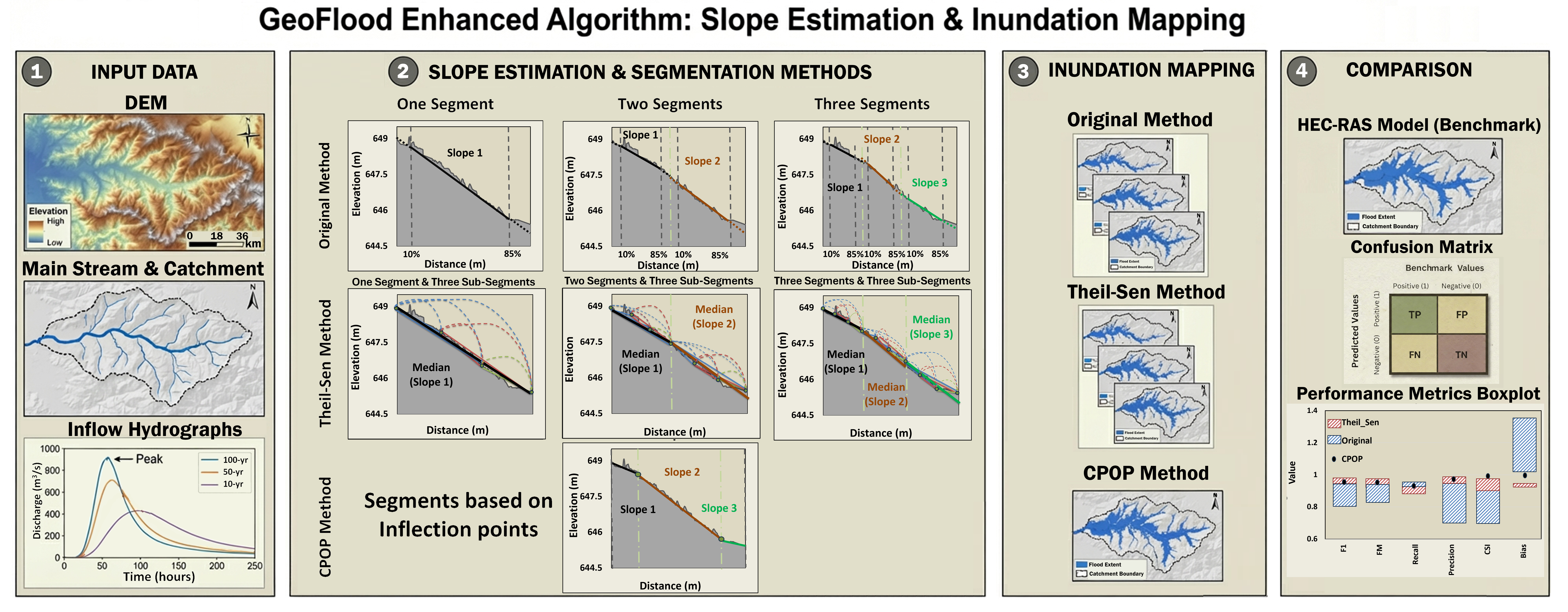
Flash floods in arid regions dictate a rapid flood inundation mapping for early warning. However, hydrodynamic models, such as HEC-RAS, provide accurate flood mapping but require extensive topographical data and high computational resources. The GeoFlood method offers a rapid alternative for early warning relying on terrain-driven framework and simple hydraulics. This study examined GeoFlood applicability on two arid catchments and tested its sensitivity for different return periods, Manning coefficients, and wadi length segmentations. The original GeoFlood method showed good consistency with HEC-RAS in well-defined wadis but relatively poor performance in flat areas, with segmentation and slope calculation significantly affecting GeoFlood accuracy and robustness. To overcome these limitations, slope calculation was improved using the Theil–Sen trend, and segmentation was automated using the penalized cost approach Continuous Piecewise Optimal Partitioning (CPOP) to detect slope breakpoints. CPOP provides superior and robust performance without prior knowledge of the best segmentation lengths, producing smoother slopes at accurate breakpoints with a Fowlkes–Mallows (FM) index of 0.88 in flat areas and an error bias of 1.05 compared to a variable FM from 0.72 to 0.88 and an error bias from 0.81 to 1.3 for the original GeoFlood. The enhanced GeoFlood provides reliable robust results in arid regions when data are scarce.

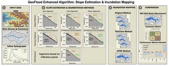
Graphical Abstract

1. Introduction

The World Economic Forum’s Global Risks Report has consistently ranked extreme weather events as one of the top global risks over the past two decades, with flooding representing one of the most hazardous climate events [1]. Rainfall-induced floods account for nearly 40% of all natural disasters worldwide, which have affected more than 3 billion people between 1990 and 2022 [2,3]. The economic losses resulting from such floods exceed USD 1.3 trillion [3,4], and future climate projections indicate substantial increases in both the frequency and intensity of extreme precipitation events [5]. As such, rainfall-driven floods should be one of the main priorities for climate adaptation, sustainable urban planning, and disaster risk reduction at national and international scales to reduce the global impact on humans, the environment, and the economy.
Arid and semi-arid regions experience rainfall-driven flooding in ways that differ fundamentally from humid climates [6]. Flash floods in these regions tend to be of short duration, are highly localized, and are exceptionally intense due to sparse vegetation cover, low infiltration capacity, crusted soils, and poorly developed natural drainage systems [7,8]. Flash floods are very hazardous, as the time for warning, evacuation, and emergency response is minimal. Recently, arid countries have experienced rapidly expanding urbanization in locations near the wadi systems based on a false sense of security due to long periods without flooding, which have amplified vulnerability in those areas [8,9]. Moreover, a single storm can trigger destructive flash floods in areas with no historical flooding due to climate change [3]. These hydrological characteristics make arid regions sensitive to extreme rainfall events projected under climate change [4,5].
The Middle East and North Africa have been experiencing increased flash flood-intensified events since the beginning of the 21st century [10,11,12]. Jeddah in Saudi Arabia experienced flash floods in 2009 and 2011; these events resulted in hundreds of fatalities and more than USD 1 billion in total [13,14]. Cyclone Gonu (2007) and Cyclone Shaheen (2021) generated catastrophic flooding, damaging infrastructure, displacing communities, and disrupting essential services in Oman [15,16,17]. Egypt has also faced repeated extreme events, specifically in the Ras Gharib area in the Red Sea governorates in 2016 and 2019, which have caused catastrophic damages to highways, oil facilities, and residential areas [8,18]. In Upper Egypt, Aswan experienced flash floods in 2021 that led to casualties, widespread property damage, and mass displacement from flooded burrows [19]. Those recurring events in arid regions urge the need for rapid high-resolution flood mapping tools to aid early-warning systems and improve land-use planning.
Flood inundation mapping has traditionally relied on empirical and statistical methods, physics-based hydrodynamic models, and, recently, machine-learning approaches [20,21]. Empirical or statistical models (i.e., regression-type analysis, stage-damage curves) have been widely used due to their simplicity and low data requirements. These approaches can only be reliable when long-term hydrologic records exist. As such, in regions with limited or no flood history, empirical and statistical methods tend to struggle with extrapolation, making them less suitable for data-scarce arid regions [21].
Hydrodynamic models, such as HEC-RAS, MIKE, LISFLOOD-FP, TUFLOW, and InfoWorks ICM, represent the physics-based approach for floodplain mapping. Such models simulate complex hydraulic behavior using 1D, 2D, or coupled 1D–2D formulations [22,23,24,25]. These models integrate the effect of inline infrastructure effects (i.e., bridges, culverts, storm-drain networks), variability in flow velocities, and spatiotemporal variations in water depth with high accuracy when properly calibrated. However, those models require extensive input data, such as high-resolution DEMs, channel geometry, roughness coefficient, hydrographs, and historical flood maps, for calibration and validation [26]. In arid and semi-arid regions where gauged flow data and observed flood extents are largely absent, calibration becomes difficult [27]. Additionally, hydrodynamic simulations can be computationally expensive, often requiring hours to days to simulate a single storm event, especially in wadis due to the huge extent of the watershed, which limits their utility for near-real-time flood forecasting or early-warning applications [28,29].
Machine-learning (ML) approaches such as Artificial Neural Networks, Convolutional Neural Networks, Random Forests, and hybrid deep-learning models have gained significant attention in recent years for flood susceptibility mapping and rapid hazard classification [30,31]. These models can capture nonlinear hydrologic behaviors and process large spatial datasets with minimal computational cost once trained. In data-rich environments, ML models have demonstrated strong predictive skills, outperforming traditional statistical methods in terms of accuracy and hydrodynamic models in terms of efficiency [28,29,32]. However, their performance is heavily dependent on the quantity and quality of training datasets, which include rainfall–runoff records with the associated flood boundaries. This requirement limits their applicability in arid regions, where flood events are infrequent, observational data are sparse, and the use of transfer-learning between basins is highly uncertain due to the unique hydrologic characteristics of wadi catchments.
Hydrodynamic models remain widely used in arid and semi-arid regions, even with limited meteorological and hydrological data; thus, the results are not reliable [33]. The produced inundation maps are highly uncertain and often rely on subjective parameter estimation due to lack of calibration. If enough data are available, hydrodynamic models are highly computationally demanding, which makes them inefficient for near real-time flood forecasting in flash flood-prone environments where response time is critical. GIS-based flood mapping techniques provide a promising and operationally feasible alternative [27,34]. These methods require minimal input data, execute within seconds to minutes, and produce first-order floodplain inundation estimates suitable for early-warning systems and preliminary risk assessments.
The Height Above Nearest Drainage (HAND) is one of the most widely adopted GIS tool models used for flood susceptibility analysis, national hazard mapping, and near-real-time inundation estimation [35,36,37]. Although HAND is computationally efficient and requires minimal hydrologic input, its performance is strongly dependent on the accuracy of the underlying drainage network and DEM quality. HAND is very sensitive to drainage lines, DEM artifacts, and channel extraction, particularly in flat terrains, braided systems, or urbanized watersheds. GeoNet was developed as an advanced terrain-processing tool to enhance the HAND tool by introducing nonlinear DEM filtering, curvature metrics, and flow-accumulation thresholds [38,39]. GeoNet substantially improves drainage-network extraction, which in turn enhances the reliability of HAND flood mapping and related terrain-driven modeling frameworks. GeoFlood emerged as a next-generation GIS-based inundation approach that synthesizes GeoNet drainage networks with HAND elevation metrics to generate synthetic rating curves for each stream reach [40,41]. A key advantage of GeoFlood is its ability to leverage GPU acceleration, allowing for the rapid processing of high-resolution DEMs across large basins with speeds far exceeding traditional hydrodynamic models. GeoFlood converts estimated discharge into water-surface elevations and inundation extents using simplified conceptual hydraulics, achieving reported match rates of 60–90% with the US Federal Emergency Management Agency (FEMA) reference flood products [37,40]. This balance of accuracy and computational efficiency positions GeoFlood as a valuable tool for emergency-response operations, large-scale regional assessments, and rapid scenario analysis.
GeoFlood is inherently more suitable for data-scarce regions, as it relies primarily on terrain characteristics rather than continuous hydrological observations. However, GeoFlood performance has not been comprehensively evaluated under arid-region conditions, and several of its core assumptions related to channel slope estimation, drainage segmentation, and DEM-derived hydraulic behavior require further investigation for flat terrain areas. The GeoFlood tool sensitivity has to be checked for uncertainties that might arise in arid regions due to limited data availability.
Accordingly, the objective of this study is to advance the understanding of GeoFlood performance in arid, data-scarce environments through two detailed case studies that (1) evaluates the accuracy of GeoFlood-generated inundation maps by comparison with a benchmark HEC-RAS 2D hydrodynamic model with different topographies; (2) investigates the sensitivity of inundation outputs to Manning coefficient, different return periods, segmentation lengths, different wadi structures, and slope-calculation methods during stream–network extraction; and finally (3) proposes two enhancements to the GeoFlood tool by incorporating a penalized cost approach (via the CPOP algorithm) to automatically detect slope breakpoints and improve the accuracy and stability of slope calculation via an alternative Theil–Sen slope trend estimation. By improving the GeoFlood tool and quantifying the resulting changes in inundation-mapping accuracy, this study provides new insights into optimizing terrain-based flood mapping for arid-region flood hazards and improving the robustness and reliability of the rapid GIS-based inundation tool GeoFlood.

2. Methods

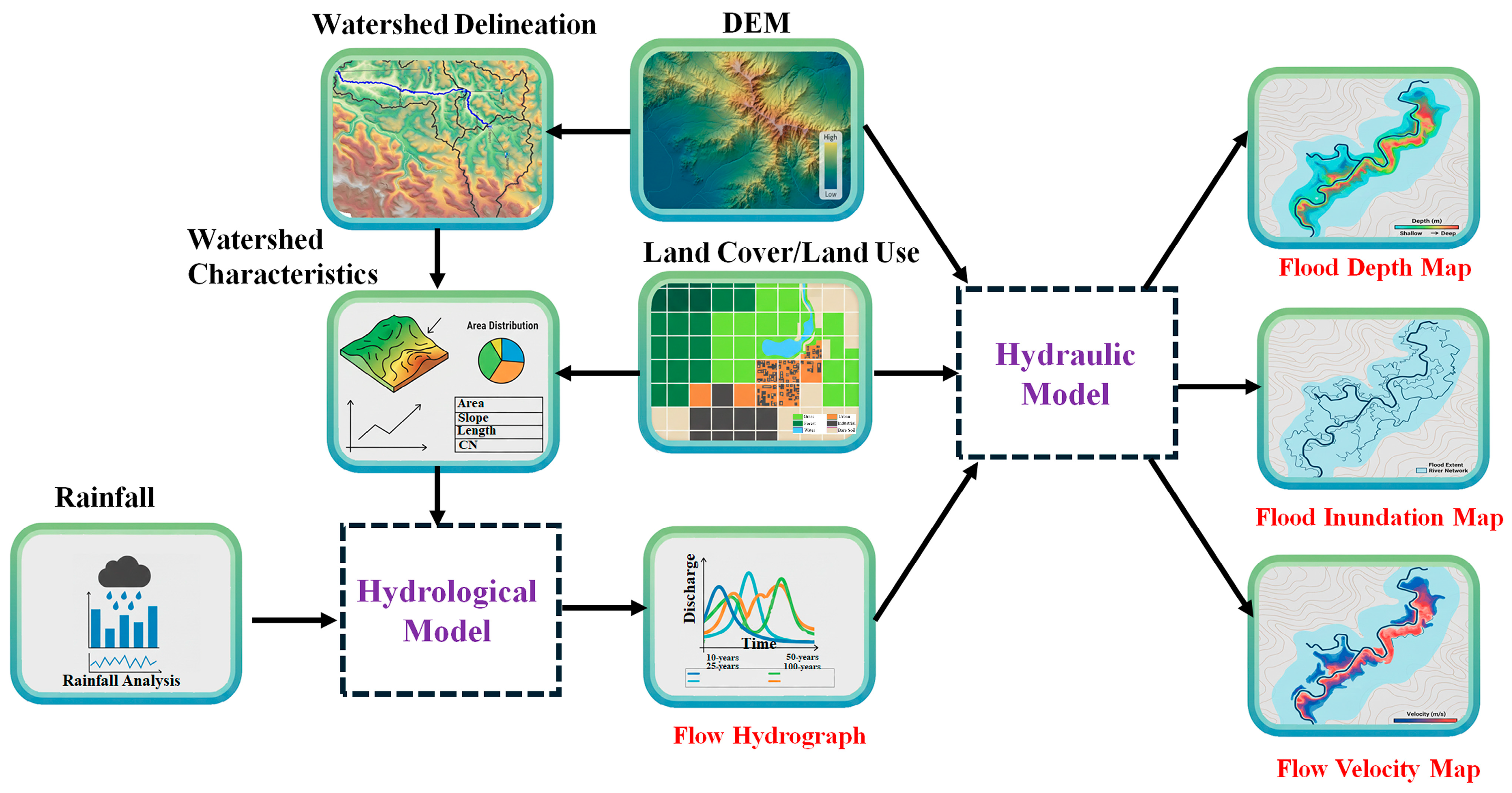
As illustrated in Figure 1, the conventional approach for generating flood inundation maps is based on coupling hydrological and hydraulic modeling. The hydrological model begins with the acquisition of a digital elevation model (DEM), land use/land cover (LULC), and rainfall data. The DEM is preprocessed to delineate the watershed at the location of interest and to extract key characteristics such as catchment area, mainstream length, and average slope. LULC is then intersected with the watershed boundary to estimate the runoff coefficient. Rainfall data are analyzed using frequency analysis and rainfall distribution curves to represent different return periods. These watershed characteristics and rainfall data are subsequently processed within a hydrological model (HEC-HMS was used in this study due to its widespread use in the literature [42,43]) to generate discharge hydrographs corresponding to each return period.
The hydraulic model uses the generated flow hydrographs together with the DEM and LULC data for the river area to simulate flood depth, velocity, and the inundation extent. Different hydraulic models can be employed, where each model uses different numerical formulations. In this case study, HEC-RAS was used as the benchmark model, which mainly relies on solving the shallow water equations. LULC in the HEC-RAS model is translated into Manning coefficients. Model performance in HEC-RAS is strongly influenced by DEM quality, Manning coefficient estimation, and computational grid resolution and direction. HEC-RAS is widely reported in the literature to produce high-accuracy results; however, it typically requires substantial data preparation and computational resources.
Both the hydrological model (HEC-HMS) and the hydraulic model (HEC-RAS) require calibration and validation; however, in arid regions where there is a lack of data measurements, the models are built based on common engineering practice, where the model’s parameters are calculated based on the code of practice and standards, then sensitivity analysis is performed [44,45,46].
In this study, the hydraulic modeling is replaced by the GIS-based tool GeoFlood to evaluate its reliability as a computationally efficient alternative for flood inundation mapping. The following subsection describes the core principles and workflow of the GeoFlood model, while the subsequent subsection presents the proposed enhancements aimed at improving GeoFlood performance and robustness.

2.1. GeoFlood Tool

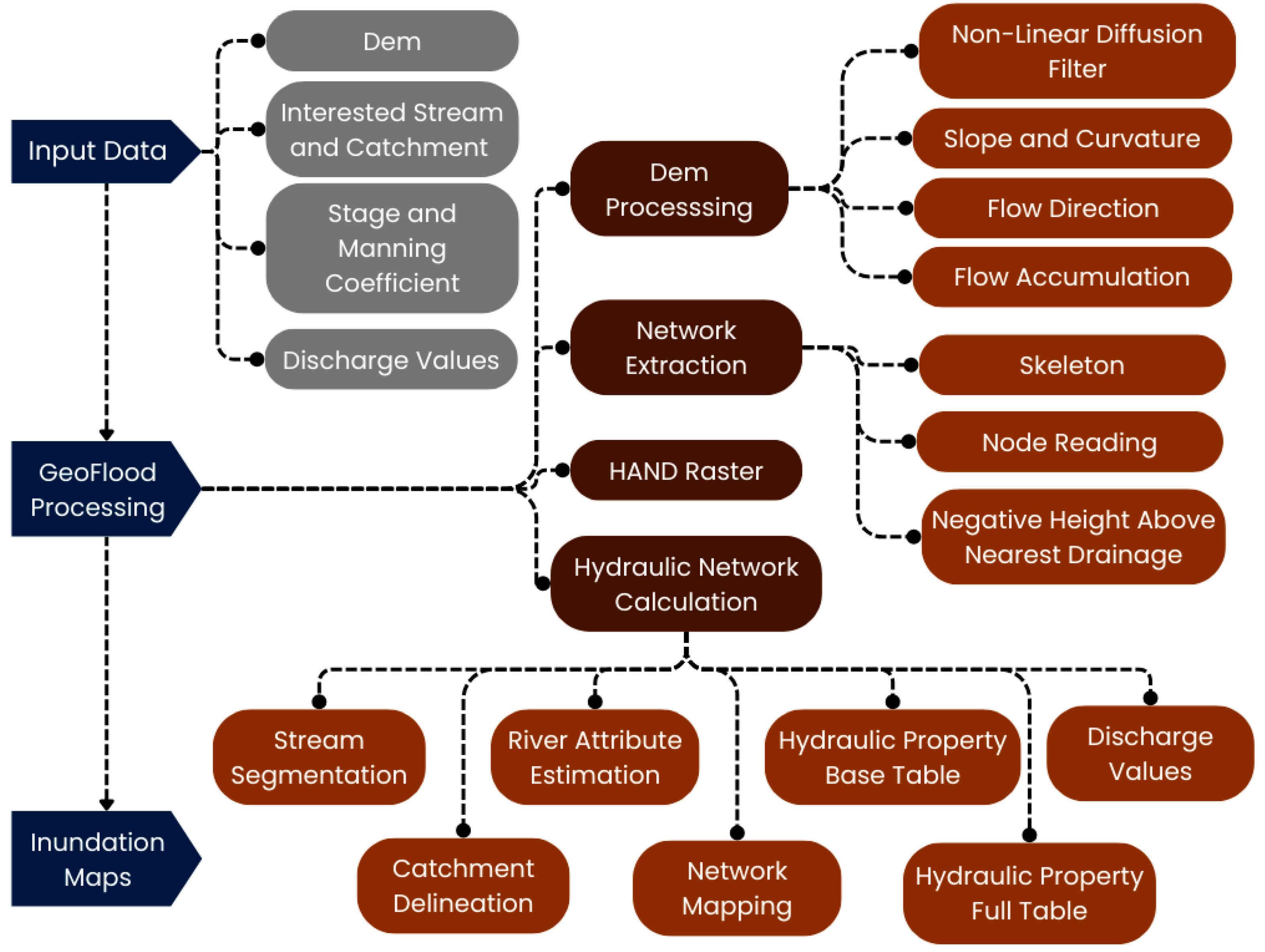
The GeoFlood tool begins with data preprocessing, which involves several critical steps: the acquisition of a high-resolution Digital Elevation Model (DEM), identification of the stream network and catchment of interest, derivation of the rating curve based on the assigned Manning coefficient, and determination of the design “hydrologic” discharge value to ensure accurate simulation [40]. The DEM provides essential information on terrain morphology, flow paths, and potential water accumulation areas [35,36]. The DEM is subsequently used for watershed delineation using the Watershed Modeling System (WMS) to define the stream network and catchment boundaries, ensuring consistency with real hydrological features. The Manning coefficient is assigned based on channel soil type/land cover to develop stage–discharge relationships. Finally, river discharge values are obtained from HEC-HMS simulations to produce the required corresponding inundation map. Following preprocessing, the GeoFlood tool is executed, encompassing four main processes: (1) DEM processing, (2) network extraction, (3) application of the HAND module, and (4) hydraulic network calculations, as shown in Figure 2.
DEM processing consists of a series of sequential steps, which begin with the application of a nonlinear diffusion filter to reduce random noise [40], and then Grass GIS is used to calculate slope, curvature, flow direction, and flow accumulation to define the path that surface water follows [47,48].
The main purpose of network extraction is to obtain a hydrologically consistent drainage network by applying a skeleton extraction to focus on the main streams, node reading for an accurate definition of start and end points to the main stream of interest, Negative Height Above Nearest Drainage (NHND) computation to identify areas located below the elevation of the nearest drainage channel and subsequently to calculate the difference between its actual elevation and the elevation of the nearest mainstream per cell, and, finally detailed hydraulic calculations such as slope, contributing area, and flow properties, which are extracted [37,40,41].
The Height Above Nearest Drainage (HAND) module is a topographic index that quantifies the vertical distance between each DEM cell and its nearest drainage cell, providing a spatial measure of relative elevation with respect to the extracted stream network [36,37]. HAND module relies on TauDEM tools for DEM processing to fill small depressions, generate flow direction and flow accumulation maps, and define drainage pathways, which is different from the original DEM processing that happened in the previous step [37,43,49]. HAND is the foundation tool for flood inundation mapping. The HAND module compares every cell’s HAND value to the simulated water surface elevation derived from rating curves and hydrologic model discharge outputs. Each grid cell is classified as inundated when its HAND value is less than or equal to the modeled water surface elevation (stage) corresponding to the simulated discharge; cells with HAND values exceeding the predicted stage are classified as non-inundated.
Hydraulic network calculations encompass several integrated steps to represent river hydraulics and flood dynamics, as shown in Figure 2. The stream of interest is divided into smaller segments to enable spatial variability in flow representation. Afterwards, catchment delineation is performed for each segment to define the contributing drainage areas. Then, river attributes such as channel length, slope, width, depth, and cross-sectional shape are calculated for each segment, where each segment is linked with its catchment by network mapping to maintain the connectivity from upstream to downstream. Finally, a hydraulic property base table and a full table detailing hydraulic relationships across multiple stage levels, such as flow area, wetted perimeter, hydraulic radius, velocity, fixed Manning coefficient, and discharge, are generated for each segment. To simulate the flood inundation map, discharge from HEC-HMS is integrated with rating curves to compute the water depth and find the flood extent. More details about GeoFlood and its operation can be found in the archived paper by Kyanjo et al. [50].

2.2. GeoFlood Slope Calculation Enhancement

GeoFlood slope estimation affects the tool performance as it controls hydraulic network calculation and river attribute estimation, which defines the critical understanding of flow dynamics and energy distribution along the channel. Slope calculation is heavily influenced by segmentation, where shorter segments yield high details but can capture local noise, while longer segments smooth out the variability, as established by Zheng et al. [37,40]. To study slope calculation sensitivity, equal segmentation was applied to the stream length, with segment lengths varying from 100 m up to the total length of the stream.
In the original GeoFlood approach, the slope of each segment was calculated using two fixed points along the segment, located at 10% and 85% of its total length. The slope was then computed as the difference in elevation between these two points divided by the cumulative distance along the segment, as shown in Equation (1) [50]. However, if the resulting slope is either zero or negative, a small positive slope (0.00001) was assigned to maintain the flow direction. All segments that were assigned this hypothetical value were rechecked with the previous segments and merged iteratively until a positive slope was obtained. Alternatively, the geometric mean of previous positive slopes could be used. While this method ensures hydrological continuity and reduces the influence of DEM noise at segment ends, it often overlooks local variations within the segment, particularly in meandering or steep areas, potentially producing unrealistic slope representations. Furthermore, it is very prone to being trapped in local erroneous elevation values.
S s e g m e n t = Z L 10 Z L 85 m L 85 m L 10
where Z L i represents the elevation at location i and mli is the cumulative distance from the beginning of the segment to that point Li.
In this study, alternative slope estimation methods were tested to enhance the original slope estimation and not to solely rely on just two points that could catch the DEM noise. Each segment is subdivided into small uniform intervals (10 m) so that the slope for each subsegment will be based on those subsegments points. Then, after computing the subsegment slopes, slope aggregation method is applied to estimate the segment slope. In this study, the average, the median, and the Theil–Sen trend method [51,52,53] were investigated. Similar assumptions were made for subsegment slopes that were adverse or zero to be replaced by (0.00001). The aggregation method using both the average and median was applied once by taking all values and another time by only considering the positive slopes while excluding assumed slope values of 0.00001. The Theil–Sen method was employed by calculating the median slope between all possible pairs of points within a segment, as shown in Equation (2). After computing the slope for each segment, the slope had to be checked with upper and lower limits based on hydrological knowledge and expert judgment to ensure a realistic tool representation for the area of interest.
S f i n a l = m e d a i n Z j Z i m j m i i < j
where Z i and Z j are elevations of points i and j, and m i and m j are their corresponding cumulative distances along the segment.
Another enhancement was introduced to the GeoFlood tool related to automatic reach segmentation based on the Continuous Piecewise Optimal Partitioning (CPOP) approach, which is a dynamic programming algorithm for detecting multiple slope breakpoints in a reach elevation profile, finding the “best” piecewise-linear fit by minimizing residual error while penalizing segmentation complexity using a penalty on changes in slope, proving a more reliable number of changepoint locations. CPOP is used in this research for both automatic segmentation and slope calculation. CPOP is different than the original GeoFlood approach as it does not rely on a prior decision on the number of segmentations or the length of segments, but the method itself identifies the optimal segmentation and the corresponding optimal slope without user/expert judgement. Nevertheless, the CPOP method divides the streams into unequal reach segments.
The CPOP approach works by extracting the longitudinal profile of the stream of interest from the DEM by sampling elevation values at regular intervals with a fixed spacing Δd (10 m is used in this study similar to other sub segmentation). Then, the CPOP approach is based on a total cost function (presented in Equation (3)) that identifies breakpoints by separating segments with different longitudinal behaviors to better represent the longitudinal profile. Those segments are found by minimizing the total cost function, which is composed of a data-fitting term and a penalty term. The penalty term is essential, as without it, the tool will treat each Δd as a new segment.
C = k = 1 k t = i k 1 t k ( z i a k d i + b k ) 2 + β k
where k is the number of longitudinal segments, t k is the breakpoint location, a k   a n d   b k are the slope and intercept of the linear representation for each segment, and β is a penalty parameter that controls segmentation sensitivity and tool complexity. The parameter β can be assumed based on the literature, then adjusted based on the output. More details are available in the Supplementary Material Appendix SA.
After identifying the breakpoints, each segment length ( L k ) is computed directly from its geometry, while the segment slope is calculated as the average rate of elevation change with respect to distance along the segment, according to Equation (4).
S l o p e k = 1 n k i = 1 n z i + 1 z Δ d i
Δ d i is the horizontal distance between consecutive points within the segment.
The CPOP approach is more representative of the river morphology than the fixed length approach because it reflects the natural downstream direction of the stream from higher to lower elevations and does not fix a priori the segmentation lengths and breakpoints locations. For more details about how the CPOP approach works, refer to Fernhead et al. [54].
All the updated codes for GeoFlood in this section are available in the data section, and the detailed explanation of the steps is in the Supplementary Material Appendix SA.

2.3. Performance Evaluation

The main focus of the inundation maps is to find the flood extent without a detailed representation of the flood depth. As such, the tool evaluation is conducted by comparing GeoFlood-generated inundation maps with either observed flood extents or benchmark hydraulic model outputs (which is what is adopted in this study) based on pixel-based comparison. This comparison relies on four quantities: True Positive (TP), False Positive (FP), False Negative (FN), and True Negative (TN), which generate a confusion matrix. Other composite metrics are derived based on these quantities. For instance, TP represents the number of pixels correctly predicted as flooded, FN corresponds to flooded pixels missed by GeoFlood, FP indicates pixels incorrectly classified as flooded, and TN describes pixels correctly identified as non-flooded. To be able to quantify the tool performance based on those four elements, composite performance metrics were used.
Most performance metrics used in the literature include precision, recall, F1-score, the Fowlkes–Mallows Index (FM), the Matthews Correlation Coefficient (MCC), accuracy, the Critical Success Index (CSI), and Error Bias (EB). Precision is a measurement of the proportion of correctly predicted flooded pixels among all predicted flooded pixels, while recall quantifies the proportion of observed flooded pixels that were correctly captured by the tool, as shown in Equations (5) and (6), respectively. F1-score represents a balance between precision and recall into a single metric, as presented in Equation (7). FM is another representation of precision and recall by evaluating the geometric mean, as shown in Equation (8). MCC is a measuring index that combines all four confusion matrix components into a balanced measure, as shown in Equation (9). Accuracy expresses the proportion of the correctly classified pixels, while CSI focuses on flooded areas by excluding TN, as shown in Equations (10) and (11), respectively. EB quantifies the tool tendency to either overestimate (EB < 1) or underestimate (EB > 1), where an EB that equals one presents no-bias perfect results, as shown in Equation (12).
P r e c i s i o n = T P T P + F P
R e c a l l = T P T P + F N
M C C = T P × T N F P × F N T P + F P × T P + F N × T N + F P × ( T N + F N )
F M = T P T P + F P × T P T P + F N
F 1 = 2 T P 2 T P + F P + F N
A c c u r a c y = T P + T N T P + T N + F P + F N
C r i t i c a l S u c c e s s I n d e x ( C S I ) = T P T P + F N + F P
E r r o r B i a s ( E B ) = F P F N
It is important to note that the extent of the evaluation boundary has a strong influence on the number of TN pixels, which can significantly inflate accuracy and affect MCC values. As such, the boundary of interest was created by applying a buffer of 1 m to the combined flood extent maps generated for each corresponding discharge related to a certain flood return period. While this approach restricts evaluation to the hydraulically relevant zones, the buffer value might still introduce a certain bias in non-flood areas. To avoid biased results, all performance metrics that include the TN value were omitted from further analysis. Precision, recall, F1-score, FM, CSI, and EB were the main performance metrics adopted in this study, as their calculation relies mainly on TP, FP, and FN, which are not sensitive to boundary buffer selection as TN is. The choice of those parameters ensures the meaningful evaluation of GeoFlood sensitivity to key parameters and its ability to reproduce benchmark flood extents.

3. Study Area

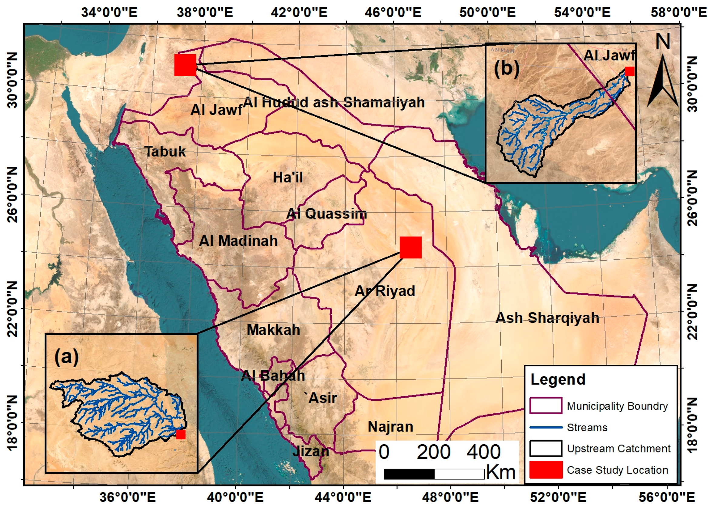
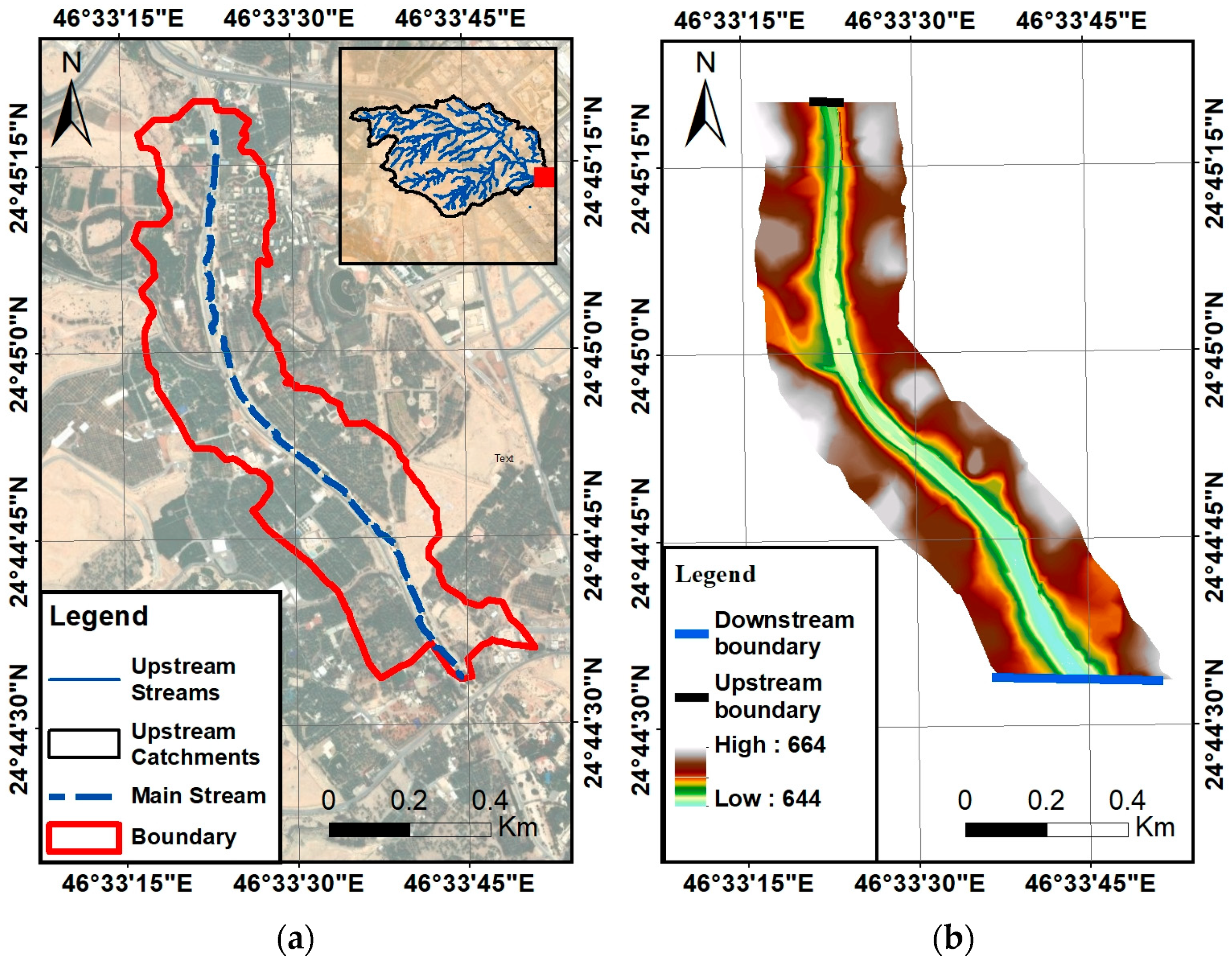
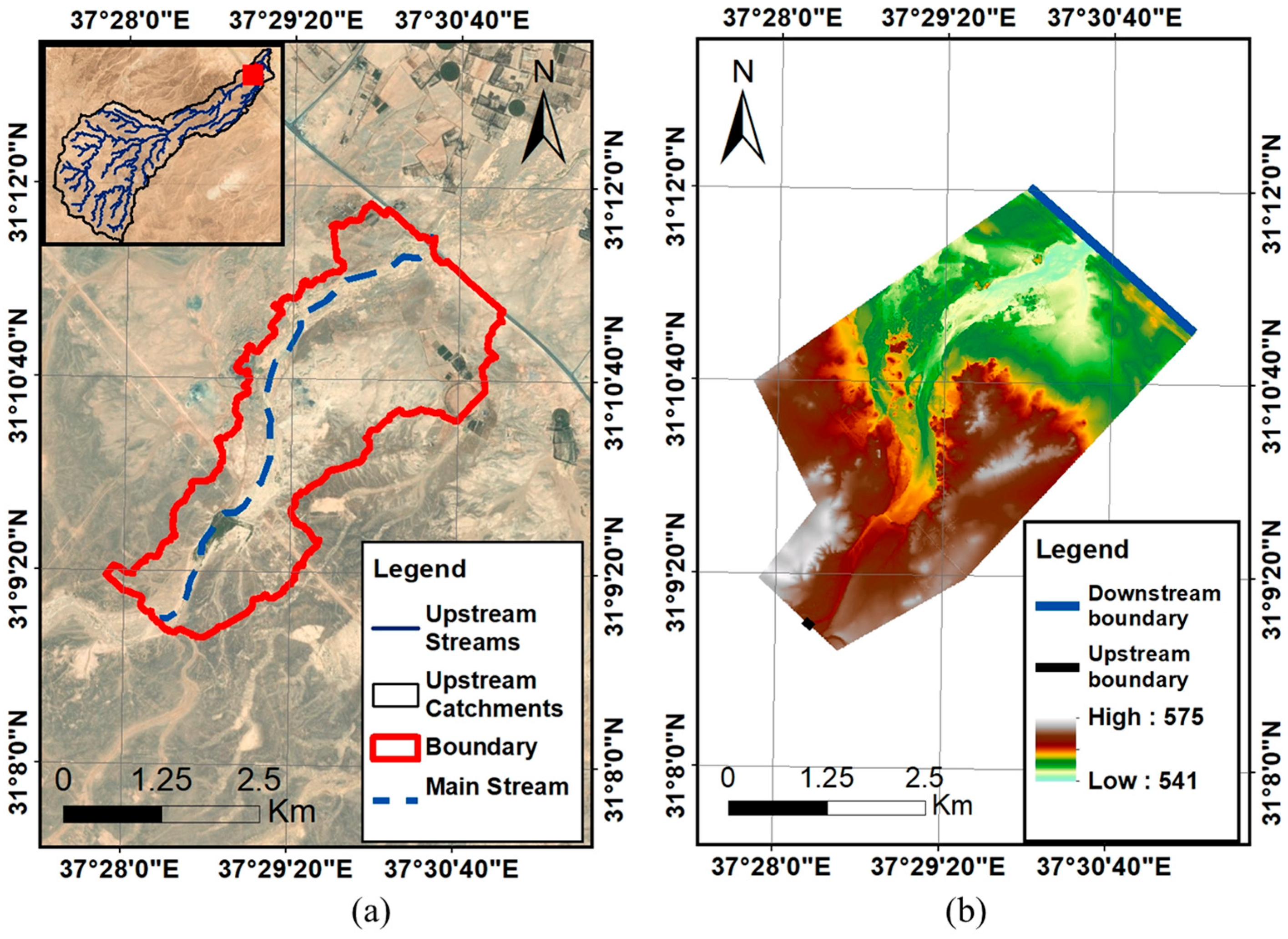
To assess GeoFlood performance and robustness in arid regions and its sensitivity to key parameters (terrain, Manning coefficient, return period), two contrasting case studies were chosen in the Kingdom of Saudi Arabia (KSA), as illustrated in Figure 3. Each case study represents distinct geomorphological and hydraulic conditions. The upstream catchments shown in Figure 3 are used to calculate the flow hydrograph using HEC-HMS. Further details are available in the Supplementary Material Appendix SB. Case Study (A) represents a section of Wadi Hanifa in Riyadh, which is represented by the red square Figure 3a. The section modeled for Wadi Hanifi is characterized by a relatively steep slope of 0.4% and a well-defined dry stream (wadi) corridor, as shown in Figure 4. Wadi Hanifa usually experiences moderate flooding, with a peak flow of 154.87 m3/s, equivalent to the 100-year return period. Case Study (B) represents the most downstream reach of Wadi Bayer located in Al-Jawf on the boundary between KSA and Jordan, as shown in Figure 3b. The reach section used in this study has slopes ranging from 0.01% to 0.3%, located within a steep mountainous region transitioning between two lowland areas, as shown in Figure 5. This reach is more complex in hydraulic conditions, as it consists of variable slopes. Wadi Bayer also experiences a higher flood discharge magnitude of 880.24 m3/s, equivalent to the 100-year storm event. GeoFlood main parameters are summarized in Table 1. Case Study (B) provides a rigorous testbed example for GeoFlood to examine its performance better under both highly dynamic flow conditions and complex stream networks.
GeoFlood performance in this manuscript was compared against the flood inundation maps generated by the hydrodynamic benchmark model (HEC-RAS 2D) according to the boundary extent shown in Figure 4b and Figure 5b, developed by Hamouda et al. [27], as there is no available flood extent or flood depth data available in this region. The HEC-RAS model is a widely accepted benchmark for flood modeling when no available measured flood data or extents are available for calibration. The HEC-RAS model had a mesh size of 3 × 3 m for Case Study (A) and 10 × 10 m for Case Study (B). The GeoFlood mesh was matched with those mesh sizes rather than the DEM resolution for comparison and consistency. More details on the HEC-HMS and HEC-RAS models, data requirements, and their sources are available in the Supplementary Material Appendix SB [55,56,57].

4. Results

This section presents the results in two main subsections. The first subsection presents an evaluation of the sensitivity of the original GeoFlood tool inundation map results to key input parameters against the benchmark HEC-RAS model results. The sensitivity analysis examines the influence of terrain (Case Study (A) and Case Study (B)), flood return periods (from 5 to 100 years), Manning coefficients (0.03–0.05), and river segmentations (fine segmentations vs. coarse segmentations). The second subsection investigates the two enhancements introduced in this study to the original GeoFlood: the robustness of results due to the alternative slope calculation method and the automatic segmentation procedure using the CPOP algorithm. All results are compared to the performance metrics of the HEC-RAS model.

4.1. GeoFlood Testing in Arid Region Context Versus HEC-RAS 2D Model

4.1.1. Sensitivity Assessment to Terrain Variation

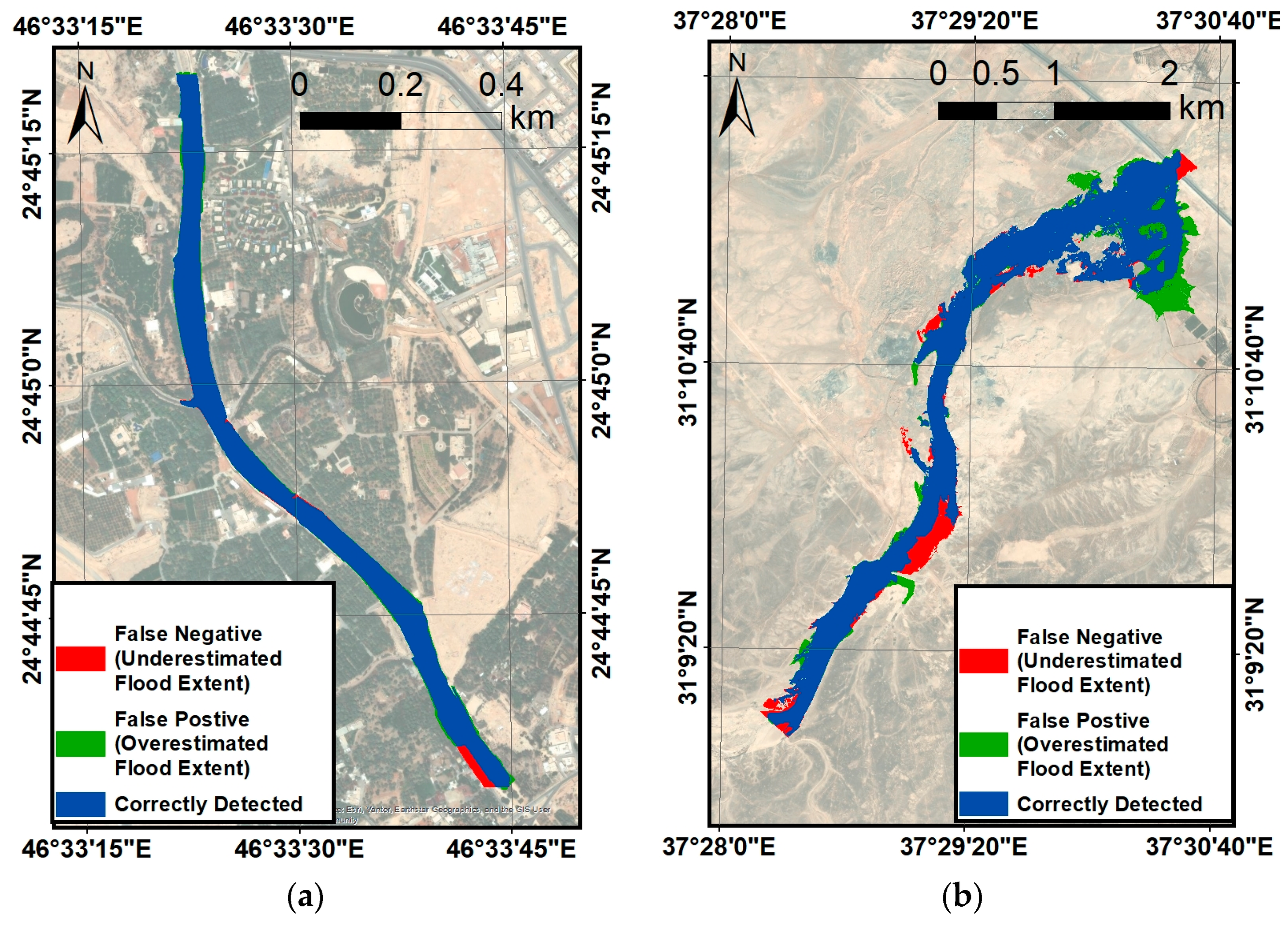
To address the terrain sensitivity, all other key parameters are kept unchanged, and only the floodplain extent due to different stream topography is assessed (Case Study (A) and Case Study (B)). The analysis was conducted for the 100-year return period flood, a Manning coefficient of 0.04, and no river segmentation. As shown in Figure 6, GeoFlood successfully reproduces the inundation extent simulated by the HEC-RAS model for Case Study (A), which is evident by the high-performance metrics reported in Table 2, with recall, precision, FM, and F1-scores all exceeding 0.95. In contrast, the GeoFlood performance for Case Study (B) is noticeably reduced, as shown in Figure 6. The recall, precision, FM, and F1-scores range from 0.85 to 0.9, which represent a clear decline relative to Case Study (A) results. The CSI metric of 0.79 and EB of 1.04 indicate an over-prediction tendency of the flood inundation map.
These results demonstrate that well-defined topographic gradients and confined wadi in the Case Study (A) allowed GeoFlood tool to detect the flood extent with high accuracy. On the other hand, the flatter terrain and weaker morphological confinement in Case Study (B) led to greater lateral spreading of water, causing overestimation of flood extent. In the absence of distinct channel boundaries, GeoFlood tends to expand inundation laterally, whereas well-defined trapezoidal or V-shaped wadis provide clearer hydraulic controls that improve the GeoFlood tool performance.

4.1.2. Sensitivity Assessment to Discharge Variation

To evaluate the sensitivity of GeoFlood to variations in discharge magnitude, the tool was assessed using the maximum discharge values corresponding to floods ranging from 5- to 100-year return periods. As the influence of terrain characteristics has already been established through the comparison between Case Study (A) and Case Study (B), the Manning coefficient was fixed at 0.04, and no river segmentation was applied. This was performed to isolate the effect of discharge magnitude on flood inundation patterns compared to the benchmark HEC-RAS model.
For Case Study (A), GeoFlood demonstrates consistently robust performance across all return period flood values, as shown in Table 3. The recall, precision, F1-score, and FM were consistently above 95%, which indicates that the GeoFlood tool was able to detect the HEC-RAS flood inundation extents accurately with minimal false detection of flooded or non-flooded areas. The bias score value remains close to one, which supports that the GeoFlood tool provides balanced results without the tendency to either overestimate or underestimate.
Case Study (B), on the contrary, experiences great variability in performance with changing the magnitude of the return period. The GeoFlood tool performance for the 5-year return period is 72% for the recall and 94% for the precision, which indicates that GeoFlood tends to prioritize minimizing false positives at the expense of underestimating the inundation extent, which is evident in the EB being 0.77. As the return period increases, the performance of GeoFlood is generally enhanced; however, for the 50-year return period, GeoFlood’s performance declines again, as shown in Table 3. GeoFlood achieves its best performance in estimating the inundation map for the 100-year return period, where recall and FM are the highest, and GeoFlood tends to slightly overestimate rather than underestimate.
These results indicate that GeoFlood is robust and will not be affected by the flood discharge value in well-defined wadis; however, in flatter terrains, the flood value plays a crucial role in GeoFlood accuracy. GeoFlood tends to give better results in high flood values; as for high-magnitude flood events, the inundation map spreads more spatially, which gives a more continuous and coherent boundary in flat terrains. However, for low to intermediate return periods, flood boundaries are highly uncertain, which affects the reliability of GeoFlood results. Consequently, the GeoFlood results in such areas require cautious interpretation as the tool tends to underestimate flood inundation extent, leaving flood-prone areas undetected.

4.1.3. Sensitivity Assessment to Manning Coefficient Variation

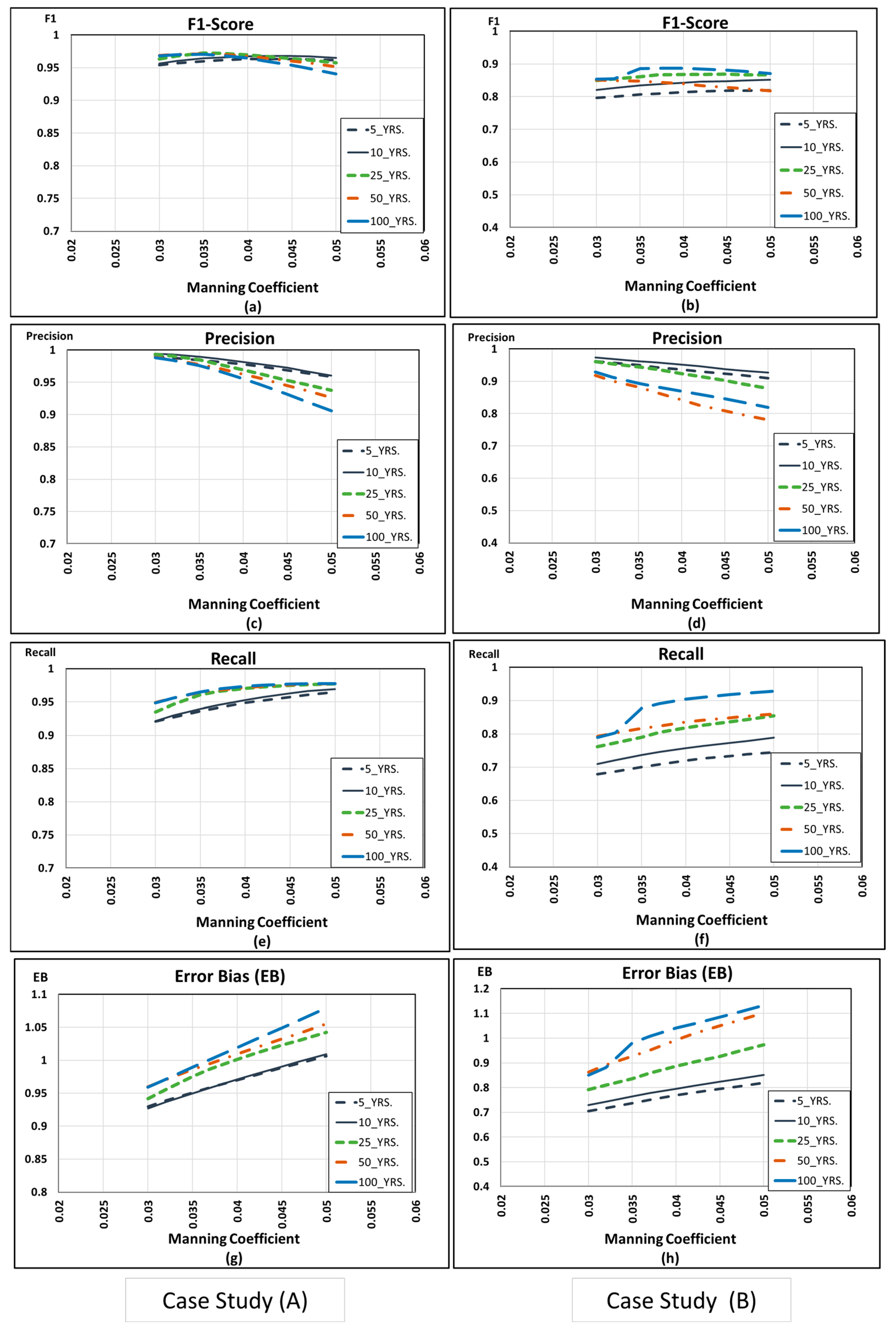
To assess the effect of the Manning coefficient, both case studies were evaluated across all return periods by changing the Manning coefficient value between 0.03 and 0.05. There was no river segmentation applied to isolate the effect of the Manning coefficient sensitivity alone. As shown in Figure 7, the F1-score is relatively insensitive to change in the Manning coefficient; however, the recall and precision values are highly sensitive in both case studies. As the Manning value increases, precision values decrease, and recall values increase for both case studies.
Case Study (B) shows higher sensitivity to the Manning coefficient compared to Case Study (A) due to terrain characteristics. As Case Study (B) is flatter and the wadi is not well defined, this amplifies the effect of the Manning coefficient on GeoFlood performance. Flow magnitude (corresponding to various return periods) also shows a strong relation to a higher sensitivity to Manning coefficient, where GeoFlood performance deteriorates as the return period increases.
These results show that the tool tends to underestimate the flood extent at low Manning coefficients and overestimate at high Manning coefficients, which is consistent given that the Manning coefficient has a direct influence on the estimated rating curve. These findings are in agreement with Zheng et al. [40], who emphasized the importance of the Manning coefficient for GeoFlood accuracy. It is worth mentioning that D’Angelo et al. [58] found that having an average Manning coefficient between wadi and overland achieved better overall performance; however, for a better representation of the inundation maps, the calibration of the Manning coefficient should be performed for different return periods to obtain a more robust error. As such, in arid regions with very scarce data, an average Manning coefficient would be a good estimate.

4.1.4. Sensitivity Assessment of Sensitivity to Stream Segmentation

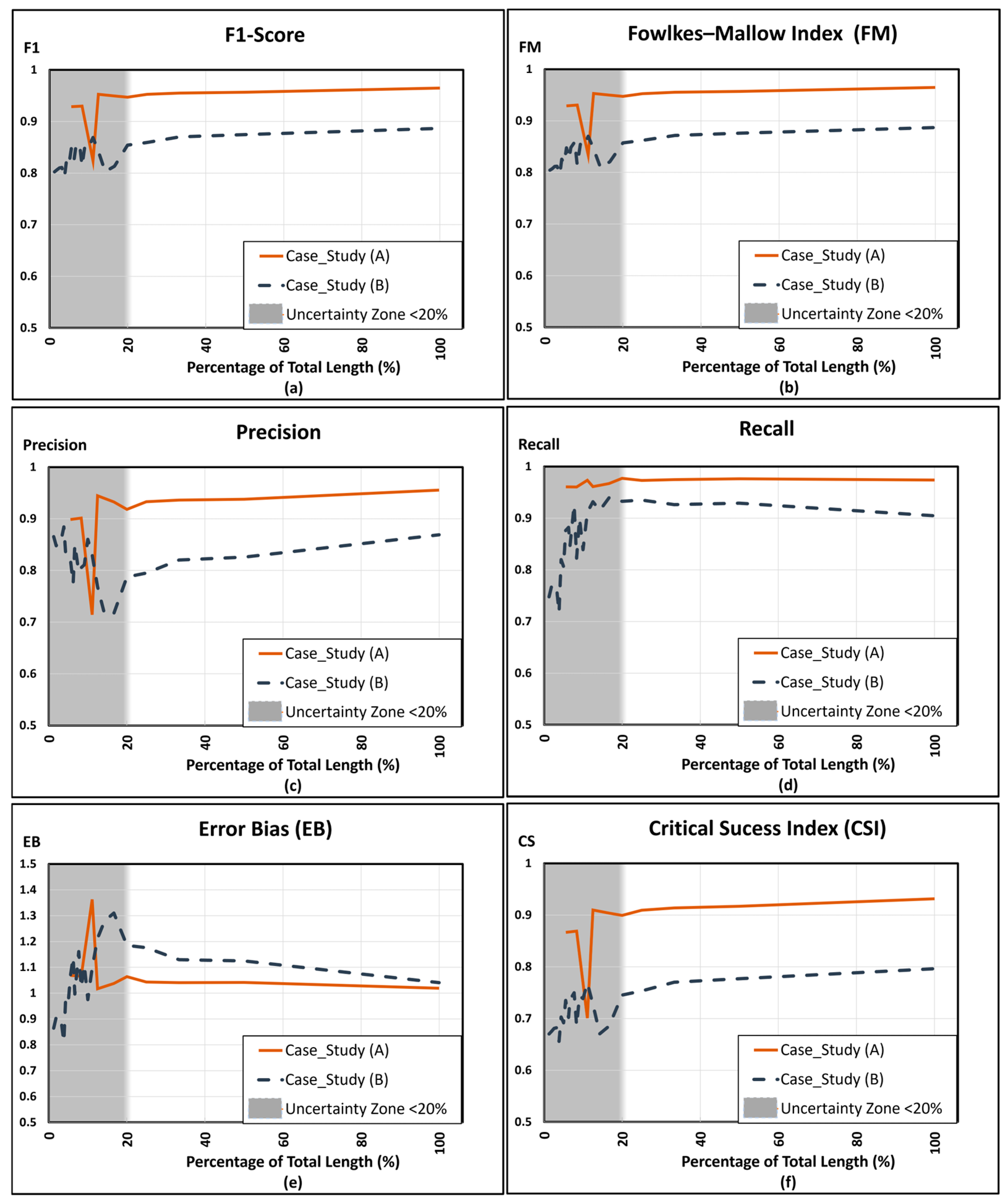
To isolate the sensitivity of GeoFlood to stream segmentation, each stream was divided into equal segments starting from a minimum segment length of 100 m and progressively increasing up to the full stream length while keeping the discharge fixed at the 100-year return period and the Manning coefficient fixed at 0.04. To allow for a consistent comparison between Case Study (A) and Case Study (B), the segmentation lengths presented in Figure 8 are expressed as a percentage of the total stream length in each study area.
As illustrated in Figure 8, GeoFlood tool performance exhibits considerable variability and inconsistency when the segmentation lengths are shorter than 20% of the total stream length in both case studies. Once the segmentation exceeds this threshold, the GeoFlood performance improves steadily. As the segmentation increased beyond 20%, the GeoFlood tool performance improved steadily. For Case Study (A), using five splits (20% of the total length) yielded an F1-score, FM, CSI, precision, recall, and EB of 0.95, 0.95, 0.9, 0.93, 0.98, and 1.06, respectively, which were enhanced to 0.97, 0.97, 0.93, 0.96, 0.97, and 1.02, respectively, when using one segment (100%). Similar results were observed in Case Study (B) beyond the 20% segmentation. Using two segments (50% of the total length) resulted in F1-score, FM, CSI, precision, recall, and bias of 0.85, 0.86, 0.75, 0.78, 0.93, and 1.18, respectively, which were enhanced to 0.89, 0.89, 0.80, 0.87, 0.91, and 1.04, respectively, when the total length was taken.
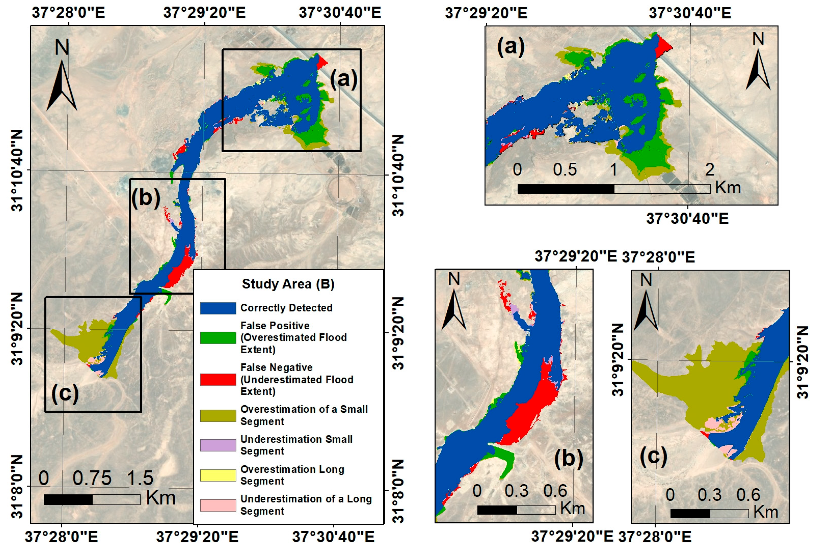
These results indicated that stream segmentations affect GeoFlood tool accuracy as tool segmentation directly affects the rating curve, which affects the HAND tool. Where shorter segments are expected to provide higher accuracy, the results showed the contrary. This is primarily due to the DEM elevation noise and the method in which GeoFlood calculates the slope for each segment. To further assess the tool’s behavior, the lowest behavior segmentation was mapped to check the flood extent. As shown in Figure 9, the GeoFlood tool with short segments overestimates the first few reaches due to the slope error calculation due to noise. As described in the methodology, GeoFlood calculates the slope using the elevation of 10% and 85% of each segment. When the segment is short, the probability that the slope is adverse or incorrect becomes higher, which explains the anomaly in Case Study (A) for the first few reaches. Even though GeoFlood corrects the slope using previous segments if the slope is too flat or adverse, the error in the first few segments is incorrect, which produces a flood extent assuming flat terrain, which is not the actual case. For Case Study (B), as shown in Figure 10, a similar pattern is observed as GeoFlood tends to overestimate at the upstream and downstream where the terrain is flatter. It is worth mentioning that the same segmentations were tested across all flood return period values and Manning coefficients, and the same conclusion was drawn that more than 20% of the total length enhanced GeoFlood performance. These observations highlight the importance of using sufficiently long segments to reduce slope estimation noise, particularly in flat and low-relief terrains.

4.2. GeoFlood Testing for Various Slope Calculation Methods and Segmentations

Since GeoFlood showed high sensitivity and unreliability in the segmentation analysis due to slope calculation errors, we investigated how to enhance GeoFlood’s slope calculation for each segment to enhance GeoFlood’s tool accuracy. This section will present our results by comparing the proposed techniques and comparing them to the original GeoFlood 10–85% slope calculation and investigating their performance against the benchmark HEC-RAS model.

4.2.1. Enhancement of Slope Calculation Method Under Equal Segmentation

These results evaluate the same equal-segmentation configurations discussed in Section 4.1.4; however, instead of relying solely on the original GeoFlood 10–85% slope calculation method, alternative slope estimators (mean positive slope, median positive slope, and Theil–Sen trend) were also tested.
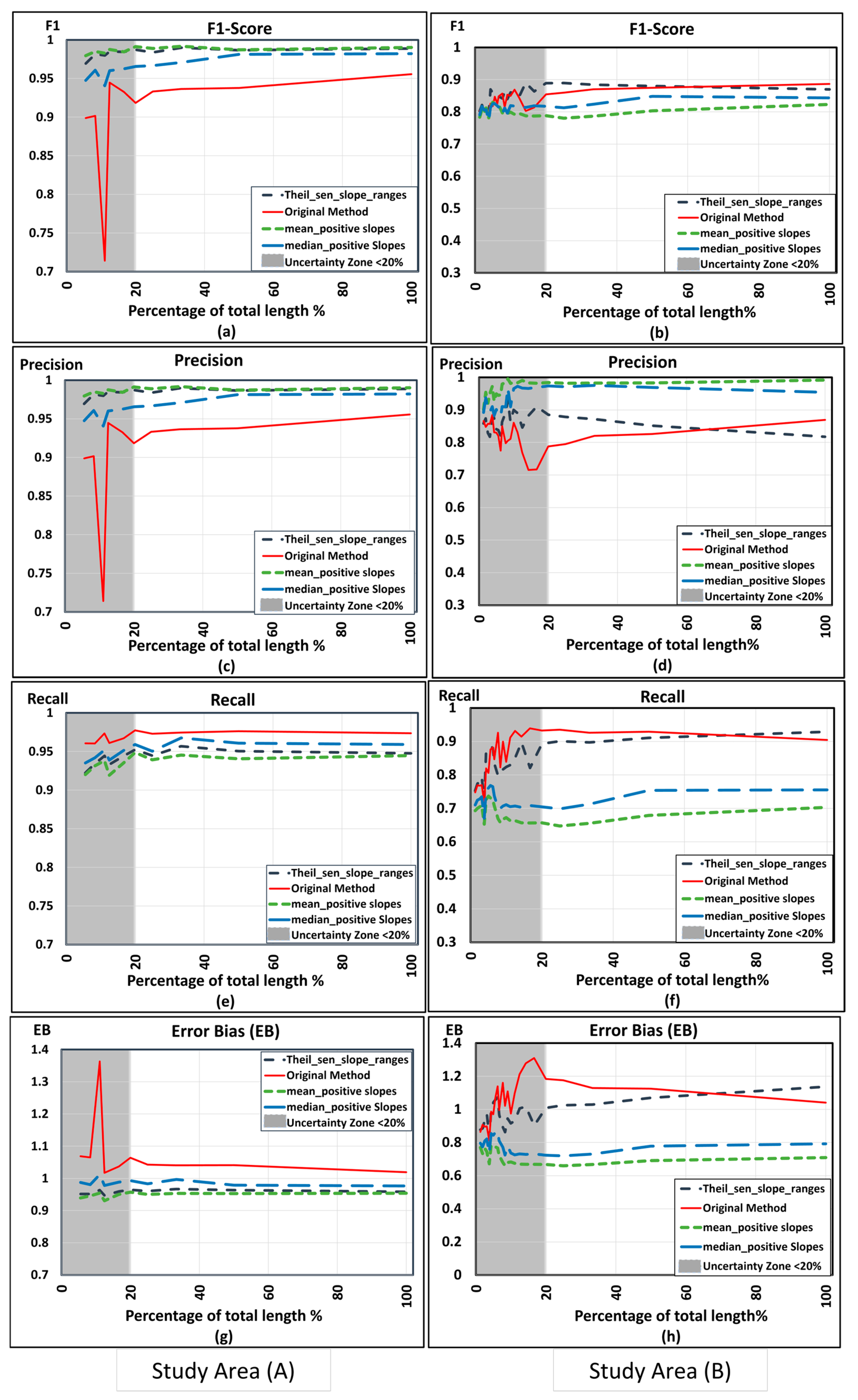
As shown in Figure 11, all alternative slope methods produced more stable and consistent performance across all segmentation lengths for Case Study (A), including segment lengths below 20% of the total stream length, where the original GeoFlood method previously showed strong inconsistency (refer to Section 4.1.4). This confirms that the performance degradation observed at small segmentation lengths is largely driven by slope estimation errors rather than segmentation itself.
For Case Study (B), no single slope method consistently outperformed the others across all segmentation percentages. The Theil–Sen method provided more consistent and generally higher accuracy than the original method for segmentation lengths below 50%. However, when no segmentation was applied (100% of the total length), the original GeoFlood 10–85% method yielded the best overall performance. The mean and median slope methods performed poorly for Case Study (B), reflecting the strong influence of terrain variability and the transition from flat to steep and back to flat wadi sections, which these methods were unable to capture adequately.
These results indicate that both the original GeoFlood slope calculation and the Theil–Sen method are sensitive to segmentation and terrain characteristics. While the Theil–Sen method is more consistent than the original method, it does not generally produce higher accuracy.

4.2.2. Enhancement of Slope Calculation Method with Automatic CPOP Segmentation

Since both the original and the Theil–Sen slope calculation methods showed sensitivity to segmentation choice and terrain characteristics, the Continuous Piecewise Optimal Partitioning (CPOP) approach was investigated as an alternative for both segmentation and slope estimation strategies. Unlike equal-length segmentation, CPOP divides the stream into uneven segments by identifying an appropriate number of breakpoints directly from the longitudinal elevation profile and then estimates an optimal representative slope for each segment by capturing the dominant terrain trends along the flow path, without applying smoothing to the original elevation values.
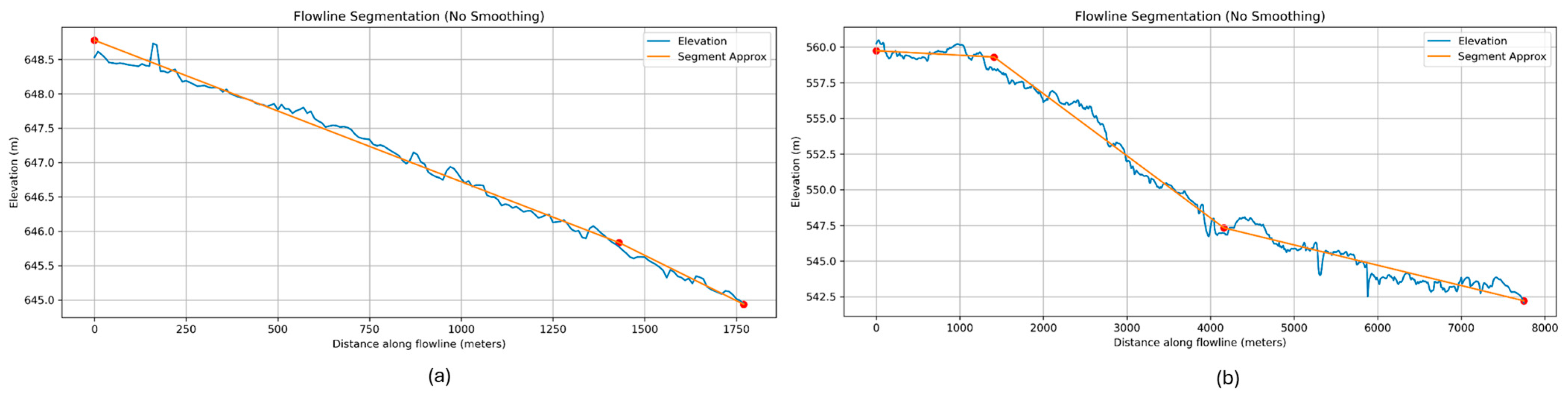
As shown in Figure 12, CPOP divided the stream in Case Study (A) into two segments. The first segment extends approximately 1300 m with an average slope of 0.23%, while the second segment covers about 300 m with an average slope of 0.3%. In Case Study (B), CPOP identified three distinct segments, where the first segment is a near-flat reach of approximately 1300 m with an average slope of 0.01%, followed by a steeper middle reach of approximately 2600 m with an average slope of 0.42% and then a final downstream segment of about 3700 m with an average slope of 0.18%. Those three segments closely represent the variation in stream terrain elevation.
The CPOP-derived segments and their corresponding slopes were then embedded within the GeoFlood tool framework to estimate the flood inundation extents. GeoFlood tool performance was evaluated against the benchmark HEC-RAS results and compared with outcomes obtained using the original slope method of GeoFlood and the Theil–Sen trend slope calculation method presented in the previous section. All comparisons are presented hereafter for the 100-year return period and a Manning coefficient of 0.04.
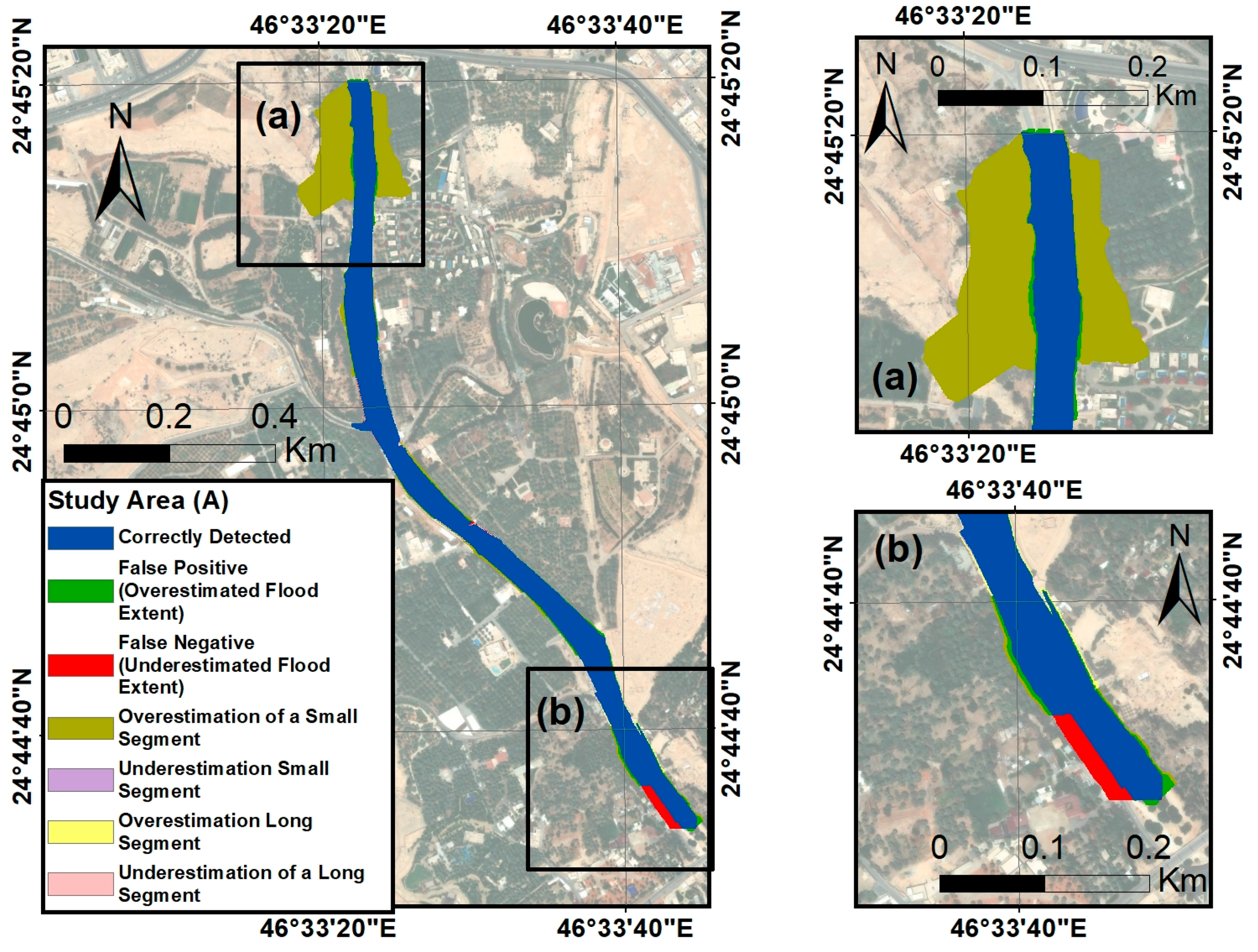
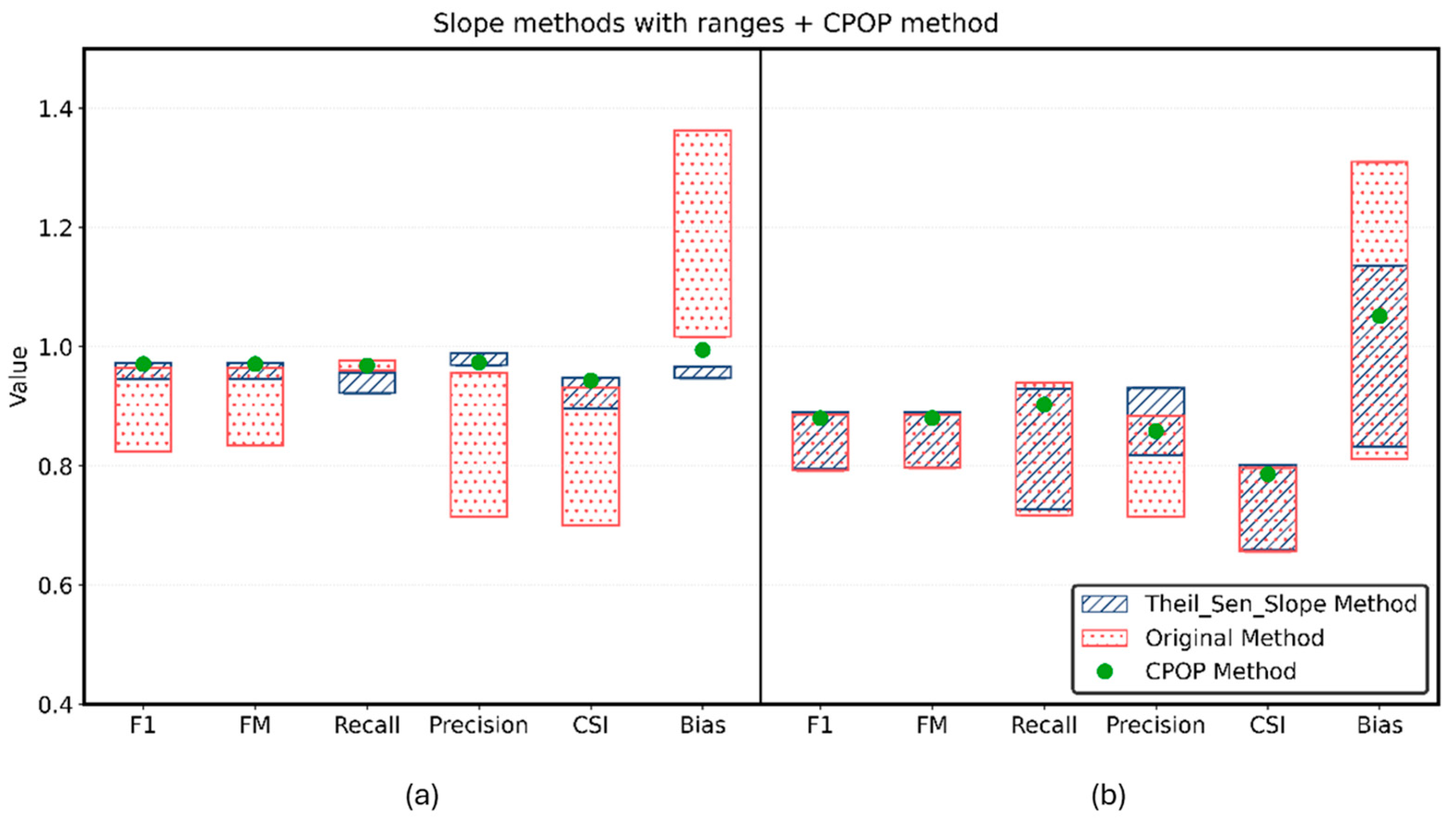
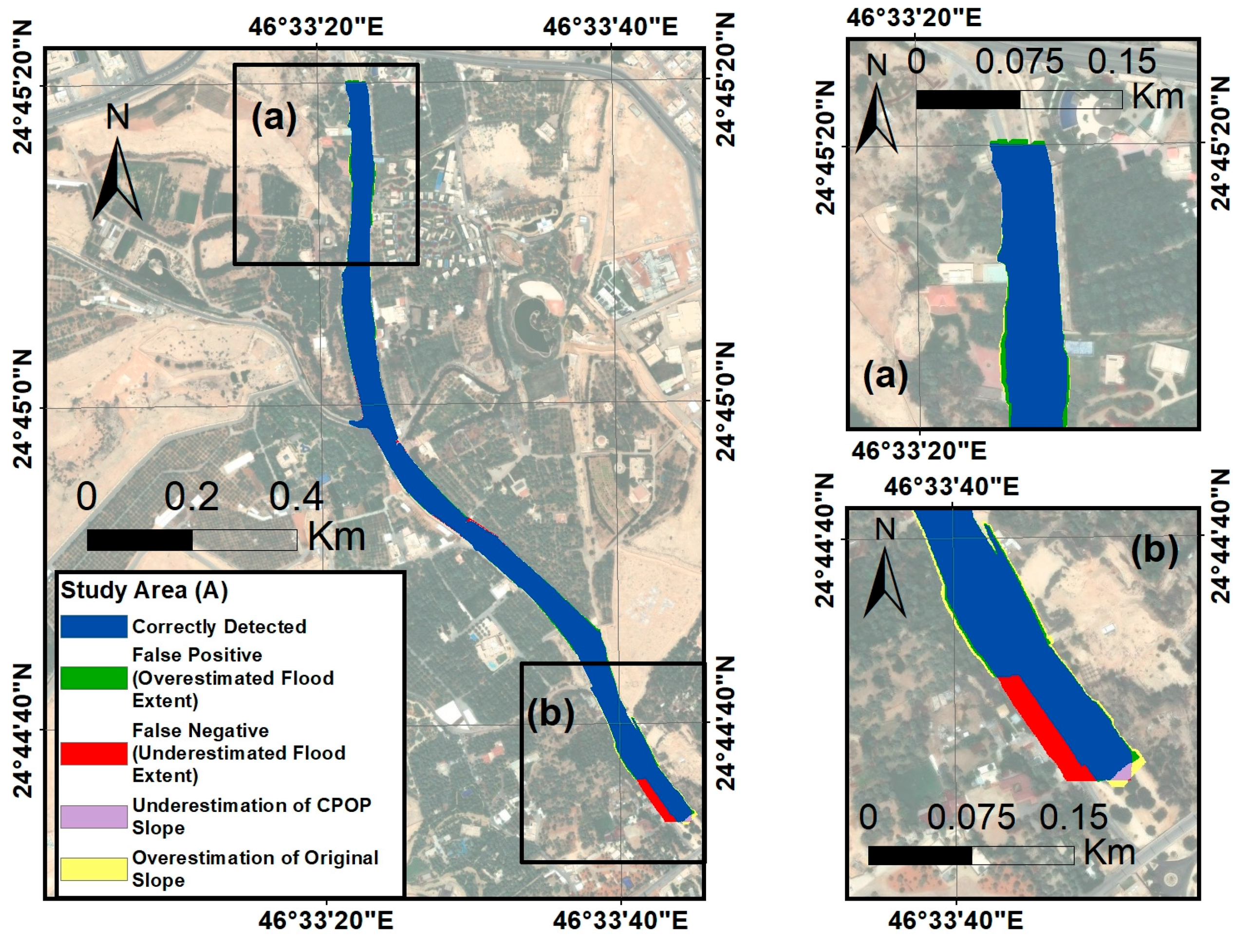
As shown in Figure 13, the CPOP method produced robust and well-balanced results for Case Study (A), with precision, recall, F1-score, FM, CSI, and EB values of 0.97, 0.97, 0.97, 0.97, 0.94, and 1.00, respectively. While the Theil–Sen method achieved similarly consistent performance, the method gave a range for each metric value depending on the used segmentation, where certain segmentations gave marginally higher accuracies. The original GeoFlood slope method showed inconsistent performance for segmentations below 20% of the total length, as previously discussed, whereas it also gave higher performance with the total length. This resulted in a wider range of performance values and occasional improvements in accuracy. Figure 14 shows a comparison between the CPOP flood inundation method compared to the best original method based on using the total segment for Case Study (A). As shown in Figure 14a, both models have the same flood extent and error, while in Figure 14b, the original method has a slight overestimation that the CPOP method does not capture.
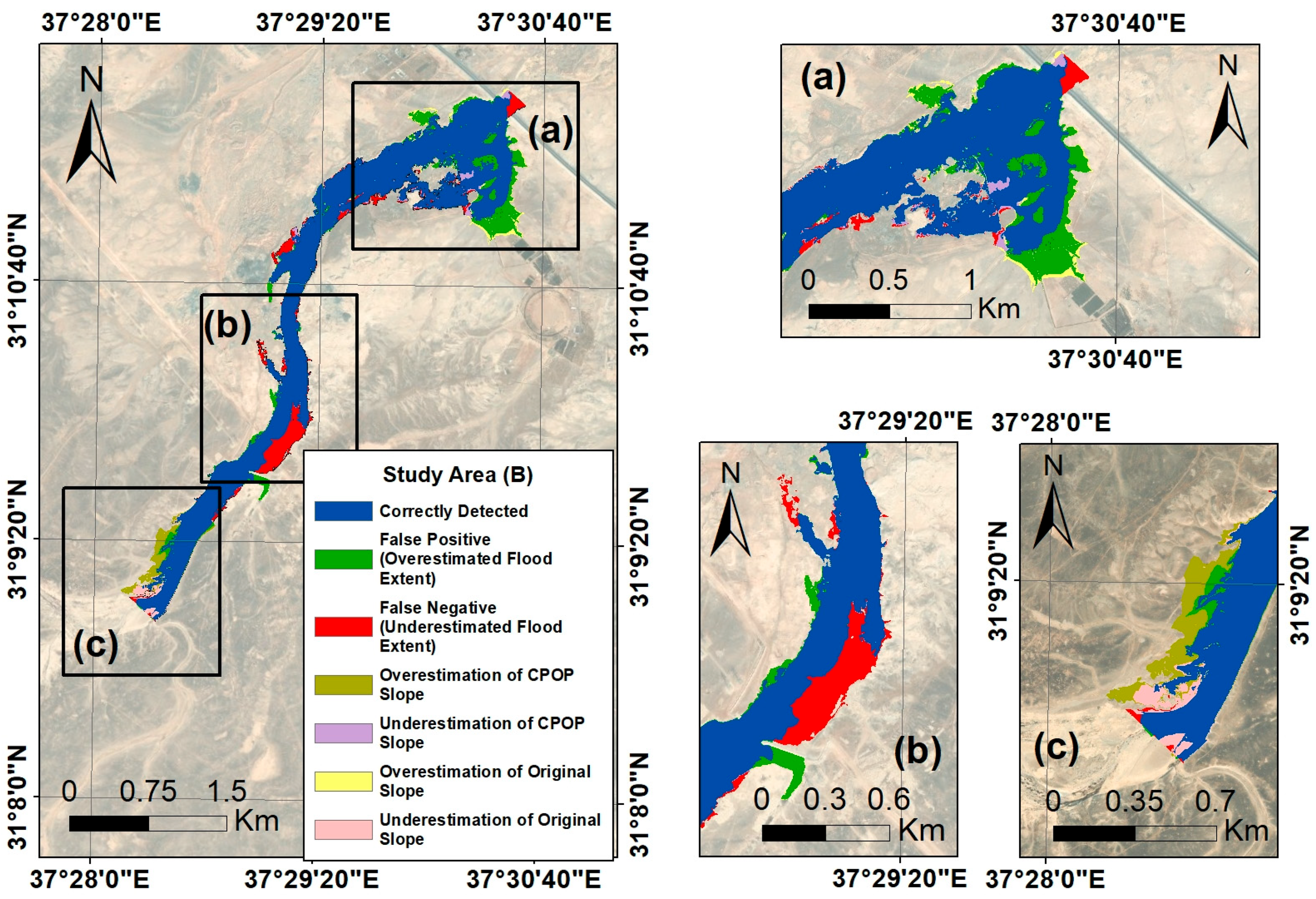
For Case Study (B), as shown in Figure 13, the CPOP method also maintained stable performance, yielding precision, recall, F1-score, FM, CSI, and EB values of 0.86, 0.91, 0.88, 0.88, 0.79, and 1.05, respectively. In contrast, both the Theil–Sen and original methods displayed higher variability with segmentation change, particularly in flat and transitional terrain sections, which led to high fluctuations in recall, precision, and bias. Figure 15 shows the comparison between the CPOP flood inundation method compared to the best original method based on using the total segment for Case Study (B). Both models have a similar flood extent; however, the original model slightly overestimates the flood extent in the downstream, as shown in Figure 15a, whereas CPOP slightly overestimates in the upstream section and the original method underestimates, as shown in Figure 15c. Everywhere else, both models have the same flood extent and error, as shown in Figure 15b.
Overall, these results indicate that the CPOP method provides the most stable and robust performance across both study areas, particularly with respect to EB, which remains close to one, suggesting that CPOP effectively mitigates the overestimation and underestimation tendencies observed in other slope calculation approaches, making it a reliable option for GeoFlood applications in heterogeneous terrain settings.

5. Discussion

This study systematically evaluated the performance of the GeoFlood tool for flood inundation mapping in arid-region environments, with a particular focus on how terrain characteristics, discharge magnitudes, Manning coefficients, stream segmentations, and slope calculation methods influence tool accuracy and stability.
Terrain characteristics were the most dominant control on GeoFlood tool performance. For Case Study (A), where the stream is well-defined wadis with clear longitudinal gradients, the tool consistently achieved excellent agreement with the benchmark HEC-RAS results, with an F1-score of more than 0.95. In contrast, flatter terrains with weak morphological confinement, as presented in Case Study (B), introduced substantial uncertainty, which led to overestimation and a substantial reduction in the F1-score to approximately 0.89. These results are in agreement with Zhen et al. (2018) [40] study that showed that HAND-based tools are less reliable in flat terrains. It is worth mentioning that the DEM resolution will affect the terrain characteristics, and as such, it is beneficial to use a high-resolution DEM, such as the one used in this study, rather than relying on low-resolution ones.
Changing return periods only affected Case Study (B), where the terrain was not well defined and where the F1-score improved from approximately 0.87 at low return periods to over 0.90 at higher return periods. This improvement reflects the fact that larger floods produce broader and more continuous inundation extents, reducing sensitivity to local elevation errors and improving boundary detectability. This bias of F1-score and CSI towards better performance in higher discharge cases is in line with previous findings from Stephens et al. (2014) [59] and Cohen et al. (2025) [60]. However, the error bias also showed that at low flow, there is a tendency of underestimation, while at high flows, GeoFlood tends to overestimate. This highlights the importance of jointly interpreting accuracy and bias rather than relying solely on a single performance metric.
The Manning coefficient was shown to be a key parameter controlling GeoFlood behavior through its influence on rating curves and HAND thresholds. For both case studies, low values tend to make the GeoFlood tool underestimate the flood extent, whereas higher values make the tool tend to overestimate, where the flatter terrain regions are mostly affected. This behavior is consistent with the expected hydraulic logic that lower Manning values result in lower water stages and higher flow velocities, producing a smaller flood extent, and vice versa. Accordingly, the sensitivity analysis aligns with theoretical explanation as well as prior studies emphasizing the need for Manning calibration and even its calibration with respect to the flood return period, as presented in the studies by Zhen et al. (2018) [37,40]. Applying spatial variable Manning coefficients along the reach would be beneficial when the land cover changes significantly; also, incorporating transverse spatial variability would be beneficial for higher flow return periods, as roughness typically differs between wadi/river and overland flow.
Stream segmentation was identified as the most critical factor affecting GeoFlood tool stability. Short segmentation lengths representing less than 20% of the total stream length consistently produced unstable results. These instabilities were primarily attributed to DEM-induced noise affecting the segment slope calculation method. When segmentation lengths exceeded 20% of the total stream length, performance improved markedly and became more consistent, with F1-scores exceeding 0.96 and CSI values surpassing 0.93. These results suggest 500 m and 2000 m as the minimum segment lengths for Case Studies (A) and (B), respectively; meanwhile, the study by Zheng et al. (2018) [40] recommended 1.5 km as the minimum segment length. Later, the study by D’Angelo et al. (2022) [58] tested lengths of 2 km, 5 km, and 10 km, and found that 5 km of a total length of 168 km indicates the best balance between inundation extent and water level accuracy. With the improvement introduced in this study by using the CPOP algorithm, there is no need to test multiple segmentation lengths in search of the optimum segmentation, as the algorithm identifies the optimum breakpoints and changes in stream slope correctly.
The Theil–Sen trend estimator and CPOP both enhanced robustness. The Theil–Sen method enhanced the original slope method, particularly for shorter segments, while the CPOP method provided the most robust and reliable performance by automatically identifying optimal segmentation locations directly from the longitudinal elevation signal. CPOP effectively eliminated the noise associated with arbitrary or overly fine segmentation. Across both study areas, CPOP achieved balanced and stable results with EB values close to 1.00 for both case studies, unlike the original and Theil–Sen methods, which poorly behaved in Case Study (B) when the segmentation was not properly selected.
This study has several limitations, as the model relied on the HEC-RAS as a benchmark instead of actual measurements due to the absence of such data. The Manning coefficient was assumed and was not calibrated, when in reality, when flow depth measurements are present, Manning calibration would give more reliable results, as both HEC-RAS and GeoFlood are sensitive to the Manning coefficient.
Future work should explore hybrid approaches that combine CPOP-based segmentation with Theil–Sen slope estimation. Additionally, embedding spatially variable Manning coefficients to better distinguish between channelized flow and overbank inundation could enhance the tool’s predictability. Moreover, CPOP–GeoFlood needs to be evaluated on longer river systems and more complex systems with multiple reaches, tributaries, and branching wadis. Such proposed research will further clarify the scalability and transferability of the proposed enhancements.

6. Conclusions

This study shows that GeoFlood can provide reliable flood inundation maps in arid environments, particularly in well-defined wadis, and maintain acceptable performance across a wide range of flood magnitudes when key parameters such as Manning coefficient and stream segmentation are properly selected. Terrain characteristics remain the dominant factor controlling GeoFlood tool accuracy where flatter areas exhibit higher sensitivity and flood extent maps are uncertain and unreliable.
Embedding the CPOP approach significantly improves the GeoFlood framework by removing the need for arbitrary segmentation and reducing errors in slope estimation. By automatically identifying terrain-driven breakpoints and representative slopes, CPOP enhances GeoFlood stability and keeps bias close to one, making the results more reliable in data-scarce regions. This makes the CPOP–GeoFlood framework well-suited for early-warning applications where detailed hydraulic models are not available. However, GeoFlood currently cannot account for hydraulic structures (such as bridges, culverts, and dams) and uses simplified conceptual hydraulics. Thus, GeoFlood cannot replace detailed hydrodynamic models like HEC-RAS in complex urban and engineering environments.
Future research should focus on the further testing and validation of the enhanced CPOP–GeoFlood framework in larger and more complex wadi systems, including areas with mixed land cover, urban environments, and microtopographic variations, and assess the model sensitivity against DEM resolution and different return periods. Comparative studies against other modeling approaches, including machine learning techniques, would also be valuable when sufficient observational data are available. Additionally, exploring the spatial variation of the Manning coefficient and the hybrid segmentation methods in more diverse hydrological and geographic contexts would be necessary.

Supplementary Materials

The following supporting information can be downloaded at: https://www.mdpi.com/article/10.3390/geomatics6010019/s1.

Author Contributions

Conceptualization, A.G.A. and N.A.A.; methodology, A.G.A. and M.G.; software, M.W.; validation, A.G.A., M.G. and M.W.; formal analysis, A.G.A.; investigation, M.W.; resources, A.G.A.; data curation, A.G.A. and M.W.; writing—original draft preparation, M.W.; writing—review and editing, A.G.A. and M.G.; visualization, M.G. and M.W.; supervision, A.G.A., M.G. and N.A.A. All authors have read and agreed to the published version of the manuscript.

Funding

This research received no external funding.

Data Availability Statement

Dataset available upon request from the authors https://github.com/marwawahba/Geoflood-Enhancement.git (accessed on 6 February 2026).

Conflicts of Interest

The authors declare no conflicts of interest.

References

  1. World Economic Forum (WEF). The Global Risks Report 2024, 19th ed.; World Economic Forum: Cologny, Switzerland, 2024. [Google Scholar]
  2. United Nations Office for Disaster Risk Reduction (UNDRR). Global Assessment Report on Disaster Risk Reduction 2023: Mapping Resilience for the Sustainable Development Goals; United Nations Publications: New York, NY, USA, 2023. [Google Scholar]
  3. Liu, Q.; Du, M.; Wang, Y.; Deng, J.; Yan, W.; Qin, C.; Liu, M.; Liu, J. Global, Regional and National Trends and Impacts of Natural Flood 1990–2022. Bull. World Health Organ. 2024, 102, 410–420. [Google Scholar] [CrossRef] [Scilit]
  4. World Meteorological Organization (WMO). WMO Atlas of Mortality and Economic Losses from Weather, Climate and Water Extremes (1970–2019); WHO: Geneva, Switzerland, 2021; Available online: https://library.wmo.int/idurl/4/57564 (accessed on 23 December 2025).
  5. Intergovernmental Panel on Climate Change (IPCC). Weather and Climate Extreme Events in a Changing Climate. In Climate Change 2021—The Physical Science Basis; Cambridge University Press: Cambridge, UK, 2023; pp. 1513–1766. [Google Scholar] [CrossRef] [Scilit]
  6. Wheater, H.; Sorooshian, S.; Sharma, K.D. Hydrological Modelling in Arid and Semi-Arid Areas; Cambridge University Press: Cambridge, UK, 2007. [Google Scholar]
  7. Borga, M.; Stoffel, M.; Marchi, L.; Marra, F.; Jakob, M. Hydrogeomorphic Response to Extreme Rainfall in Headwater Systems: Flash Floods and Debris Flows. J. Hydrol. 2014, 518, 194–205. [Google Scholar] [CrossRef] [Scilit]
  8. Arnous, M.O.; El-Rayes, A.E.; El-Nady, H.; Helmy, A.M. Flash Flooding Hazard Assessment, Modeling, and Management in the Coastal Zone of Ras Ghareb City, Gulf of Suez, Egypt. J. Coast. Conserv. 2022, 26, 26–77. [Google Scholar] [CrossRef] [Scilit]
  9. Oroud, I.M. The Relative Impact of Urbanization Expansion and Climate Change on Flood Hazard in Amman City. Jordan J. Earth Environ. Sci. 2025, 1, 96–107. [Google Scholar]
  10. Almazroui, M.; Saeed, S.; Saeed, F.; Islam, M.N.; Ismail, M. Projections of Precipitation and Temperature over the South Asian Countries in CMIP6. Earth Syst. Environ. 2020, 4, 297–320. [Google Scholar] [CrossRef] [Scilit]
  11. Loudyi, D.; Kantoush, S.A. Flood Risk Management in the Middle East and North Africa (MENA) Region. Urban Water J. 2020, 17, 379–380. [Google Scholar] [CrossRef] [Scilit]
  12. Zittis, G.; Almazroui, M.; Alpert, P.; Ciais, P.; Cramer, W.; Dahdal, Y.; Fnais, M.; Francis, D.; Hadjinicolaou, P.; Howari, F.; et al. Climate Change and Weather Extremes in the Eastern Mediterranean and Middle East. Rev. Geophys. 2022, 60, e2021RG000762. [Google Scholar] [CrossRef] [Scilit]
  13. Youssef, A.M.; Pradhan, B.; Sefry, S.A. Flash Flood Susceptibility Assessment in Jeddah City (Kingdom of Saudi Arabia) Using Bivariate and Multivariate Statistical Models. Environ. Earth Sci. 2016, 75, 12. [Google Scholar] [CrossRef] [Scilit]
  14. Ameur, F. Floods in Jeddah, Saudi Arabia: Unusual Phenomenon and Huge Losses. What Prognoses. In 3rd European Conference on Flood Risk Management (FLOODrisk 2016); E3S Web of Conferences: Les Ulis Cedex A, France, 2016; Volume 7. [Google Scholar] [CrossRef] [Scilit]
  15. Al-Awadhi, T.; Al-Awadhi, K.; Al-Awadhi, H.; Al Nasiri, N.; Abulibdeh, A.; El Kenawy, A. An Exploratory Assessment of Cyclone Risk Perceptions in Oman: A Snowball Sampling Study of Community Awareness. Sustain. Futures 2025, 10, 101335. [Google Scholar] [CrossRef] [Scilit]
  16. Al-Shaqsi, S. Care or Cry: Three Years from Cyclone Gonu. What Have We Learnt? Oman Med. J. 2010, 25, 162–167. [Google Scholar] [CrossRef] [Scilit] [PubMed]
  17. Joseph, M.A.; Natarajan, J.; Al Farsi, T.K.; Al Saifi, A.Z.M.; Al Saidi, W.K.; Al Jassassi, O.A.; Al Mukhaini, H.M. The Impact of the 2021 Cyclone Shaheen on the Mental Health of Affected Omanis. Oman Med. J. 2023, 38, e483. [Google Scholar] [CrossRef] [Scilit]
  18. Abuzeid, T.S.; Ashour, M.A.; Mahmoud, H. Documenting and Analyzing the Harmful Impacts of the Seasonal Floods in Upper Egypt on Qena-Safaga Railway Track Infrastructure. J. Eng. Sci. 2022, 50, 292–311. [Google Scholar] [CrossRef] [Scilit]
  19. Abuzied, S.; Yuan, M.; Ibrahim, S.; Kaiser, M.; Saleem, T. Geospatial Risk Assessment of Flash Floods in Nuweiba Area, Egypt. J. Arid Environ. 2016, 133, 54–72. [Google Scholar] [CrossRef] [Scilit]
  20. Teng, J.; Jakeman, A.J.; Vaze, J.; Croke, B.F.W.; Dutta, D.; Kim, S.S.H. Flood Inundation Modelling: A Review of Methods, Recent Advances and Uncertainty Analysis. Environ. Model. Softw. 2017, 90, 201–216. [Google Scholar] [CrossRef] [Scilit]
  21. Sivapalan, M.; Takeuchi, K.; Franks, S.W.; Gupta, V.K.; Karambiri, H.; Lakshmi, V.; Liang, X.; McDonnell, J.J.; Mendiondo, E.M.; O’Connell, P.E.; et al. IAHS Decade on Predictions in Ungauged Basins (PUB), 2003–2012: Shaping an Exciting Future for the Hydrological Sciences. Hydrol. Sci. J. 2003, 48, 857–880. [Google Scholar] [CrossRef] [Scilit]
  22. Jafarzadegan, K.; Abbaszadeh, P.; Moradkhani, H. Sequential Data Assimilation for Real-Time Probabilistic Flood Inundation Mapping. Hydrol. Earth Syst. Sci. 2021, 25, 4995–5011. [Google Scholar] [CrossRef] [Scilit]
  23. Oliva, A.; Olcina, J. Hydraulic Capacity of the Segura River Channel (SE Spain) in Urban Areas: 2D Hydraulic Modeling in HEC-RAS and Comparison of Results with the September 2019 Flood Event in the Lower Segura Basin. GeoHazards 2025, 6, 77. [Google Scholar] [CrossRef] [Scilit]
  24. Crenganis, L.M.; Pricop, C.I.; Diac, M.; Olteanu-Raimond, A.M.; Loghin, A.M. Flood Risk Prediction and Management by Integrating GIS and HEC-RAS 2D Hydraulic Modelling: A Case Study of Ungheni, Iasi County, Romania. Water 2025, 17, 2959. [Google Scholar] [CrossRef] [Scilit]
  25. Oluwadare, T.S.; Chen, D.; Mcgrath, H. Integrating Remote Sensing Indices and Ensemble Machine Learning Model with Independent HEC-RAS 2D Model for Enhanced Flood Prediction and Risk Assessment in the Oawa River Watershed. Appl. Sci. 2025, 2026, 70. [Google Scholar] [CrossRef] [Scilit]
  26. Shu, X.; Ye, C.; Xu, Z.; Liao, R.; Song, P.; Zhang, S. An Enhanced Framework for Assessing Pluvial Flooding Risk with Integrated Dynamic Population Vulnerability at Urban Scale. Remote Sens. 2025, 17, 654. [Google Scholar] [CrossRef] [Scilit]
  27. Hamouda, M.A.; Awadallah, A.G.; Abdel-Maguid, R.H. Extension of the Geomorphic Flood Index Classifier to Predict Flood Inundation Maps for Uncalibrated Rainfall Depths in Arid Regions. Nat. Hazards 2024, 120, 4633–4655. [Google Scholar] [CrossRef] [Scilit]
  28. Ghaith, M.; Yosri, A.; El-Dakhakhni, W. Synchronization-Enhanced Deep Learning Early Flood Risk Predictions: The Core of Data-Driven City Digital Twins for Climate Resilience Planning. Water 2022, 14, 3619. [Google Scholar] [CrossRef] [Scilit]
  29. Yosri, A.; Ghaith, M.; El-Dakhakhni, W. Deep Learning Rapid Flood Risk Predictions for Climate Resilience Planning. J. Hydrol. 2024, 631, 130817. [Google Scholar] [CrossRef] [Scilit]
  30. Bentivoglio, R.; Isufi, E.; Jonkman, S.N.; Taormina, R. Deep Learning Methods for Flood Mapping: A Review of Existing Applications and Future Research Directions. Hydrol. Earth Syst. Sci. 2022, 26, 4345–4378. [Google Scholar] [CrossRef] [Scilit]
  31. Hou, J.; Li, X.; Bai, G.; Wang, X.; Zhang, Z.; Yang, L.; Du, Y.; Ma, Y.; Fu, D.; Zhang, X. A Deep Learning Technique Based Flood Propagation Experiment. J. Flood Risk Manag. 2021, 14, e12718. [Google Scholar] [CrossRef] [Scilit]
  32. He, Z.; Chen, Y.; Ning, Q.; Lu, B.; Xie, S.; Tang, S. Unraveling Nonlinear and Spatially Heterogeneous Impacts of Urban Pluvial Flooding Factors in a Hill-Basin City Using Geographically Explainable Artificial Intelligence: A Case Study of Changsha. Sustainability 2025, 17, 9866. [Google Scholar] [CrossRef] [Scilit]
  33. Abdelshafy, M.; Mostafa, A. Flash Flood Modeling Using HEC-RAS (2D) Model on Wadi Reem in the Western Region, Kingdom of Saudi Arabia. J. Egypt. Acad. Soc. Environ. Dev. 2021, 22, 17–32. [Google Scholar] [CrossRef] [Scilit]
  34. Calapini, W.D.; Tan, F.J.; Monjardin, C.E.F.; Gacu, J.G. Geospatial Analysis of Flood Hazard Using GIS-Based Hydrologic–Hydraulic Modeling: A Case of the Cagayan River Basin, Philippines. Geomatics 2025, 5, 64. [Google Scholar] [CrossRef] [Scilit]
  35. Nobre, A.D.; Cuartas, L.A.; Hodnett, M.; Rennó, C.D.; Rodrigues, G.; Silveira, A.; Waterloo, M.; Saleska, S. Height Above the Nearest Drainage—A Hydrologically Relevant New Terrain Model. J. Hydrol. 2011, 404, 13–29. [Google Scholar] [CrossRef] [Scilit]
  36. Rennó, C.D.; Nobre, A.D.; Cuartas, L.A.; Soares, J.V.; Hodnett, M.G.; Tomasella, J.; Waterloo, M.J. HAND, a New Terrain Descriptor Using SRTM-DEM: Mapping Terra-Firme Rainforest Environments in Amazonia. Remote Sens. Environ. 2008, 112, 3469–3481. [Google Scholar] [CrossRef] [Scilit]
  37. Zheng, X.; Tarboton, D.G.; Maidment, D.R.; Liu, Y.Y.; Passalacqua, P. River Channel Geometry and Rating Curve Estimation Using Height above the Nearest Drainage. J. Am. Water Resour. Assoc. 2018, 54, 785–806. [Google Scholar] [CrossRef] [Scilit]
  38. Passalacqua, P.; Do Trung, T.; Foufoula-Georgiou, E.; Sapiro, G.; Dietrich, W.E. A Geometric Framework for Channel Network Extraction from Lidar: Nonlinear Diffusion and Geodesic Paths. J. Geophys. Res. Earth Surf. 2010, 115. [Google Scholar] [CrossRef] [Scilit]
  39. Passalacqua, P.; Belmont, P.; Foufoula-Georgiou, E. Automatic Geomorphic Feature Extraction from Lidar in Flat and Engineered Landscapes. Water Resour. Res. 2012, 48. [Google Scholar] [CrossRef] [Scilit]
  40. Zheng, X.; Maidment, D.R.; Tarboton, D.G.; Liu, Y.Y.; Passalacqua, P. GeoFlood: Large-Scale Flood Inundation Mapping Based on High-Resolution Terrain Analysis. Water Resour. Res. 2018, 54, 10013–10033. [Google Scholar] [CrossRef] [Scilit]
  41. Garousi-Nejad, I.; Tarboton, D.G.; Aboutalebi, M.; Torres-Rua, A.F. Terrain Analysis Enhancements to the Height Above Nearest Drainage Flood Inundation Mapping Method. Water Resour. Res. 2019, 55, 7983–8009. [Google Scholar] [CrossRef] [Scilit]
  42. Odey, G.; Cho, Y. Event-Based vs. Continuous Hydrological Modeling with HEC-HMS: A Review of Use Cases, Methodologies, and Performance Metrics. Hydrology 2025, 12, 39. [Google Scholar] [CrossRef] [Scilit]
  43. Tesfa, T.K.; Tarboton, D.G.; Watson, D.W.; Schreuders, K.A.; Baker, M.E.; Wallace, R.M. Extraction of Hydrological Proximity Measures from DEMs Using Parallel Processing. Environ. Model. Softw. 2011, 26, 1696–1709. [Google Scholar] [CrossRef] [Scilit]
  44. Abdessamed, D.; Abderrazak, B. Coupling HEC-RAS and HEC-HMS in Rainfall–Runoff Modeling and Evaluating Floodplain Inundation Maps in Arid Environments: Case Study of Ain Sefra City, Ksour Mountain. SW of Algeria. Environ. Earth Sci. 2019, 78, 586. [Google Scholar] [CrossRef] [Scilit]
  45. Vojtek, M.; Petroselli, A.; Vojteková, J.; Asgharinia, S. Flood Inundation Mapping in Small and Ungauged Basins: Sensitivity Analysis Using the EBA4SUB and HEC-RAS Modeling Approach. Hydrol. Res. 2019, 50, 1002–1019. [Google Scholar] [CrossRef] [Scilit]
  46. Papaioannou, G.; Varlas, G.; Terti, G.; Papadopoulos, A.; Loukas, A.; Panagopoulos, Y.; Dimitriou, E. Flood Inundation Mapping at Ungauged Basins Using Coupled Hydrometeorological-Hydraulic Modelling: The Catastrophic Case of the 2006 Flash Flood in Volos City, Greece. Water 2019, 11, 2328. [Google Scholar] [CrossRef] [Scilit]
  47. Neteler, M.; Bowman, M.; Landa, M.; Metz, M. GRASS GIS: A Multi-Purpose Open Source GIS. Environ. Model. Softw. 2012, 31, 124–130. [Google Scholar] [CrossRef] [Scilit]
  48. Chlumsky, R.; Craig, J.R.; Tolson, B.A. A Reach-Integrated Hydraulic Modelling Approach for Large-Scale and Real-Time Inundation Mapping. Geosci. Model Dev. 2025, 18, 3387–3403. [Google Scholar] [CrossRef] [Scilit]
  49. Tarboton, D.G. A New Method for the Determination of Flow Directions and Upslope Areas in Grid Digital Elevation Models. Water Resour. Res. 1997, 33, 309–319. [Google Scholar] [CrossRef] [Scilit]
  50. Kyanjo, B. GeoFlood: Computational Model for Overland Flooding. Ph.D. Thesis, Boise State University, Boise, ID, USA, 2023. Available online: https://scholarworks.boisestate.edu/td/2290/ (accessed on 6 February 2026).
  51. Chervenkov, H.; Slavov, K. Theil–Sen Estimator vs. Ordinary Least Squares—Trend Analysis for Selected ETCCDI Climate Indices. Comptes Rendus L’Academie Bulg. Sci. 2019, 72, 47–54. [Google Scholar] [CrossRef] [Scilit]
  52. Theil, H. A Rank-Invariant Method of Linear and Polynomial Regression Analysis. In Henri Theil’s Contributions to Economics and Econometrics; Advanced Studies in Theoretical and Applied Econometrics; Springer: Dordrecht, The Netherlands, 1992; Volume 23. [Google Scholar] [CrossRef] [Scilit]
  53. Sen, P.K. Estimates of the Regression Coefficient Based on Kendall’s Tau. J. Am. Stat. Assoc. 1968, 63, 1379–1389. [Google Scholar] [CrossRef]
  54. Fearnhead, P.; Maidstone, R.; Letchford, A. Detecting Changes in Slope with an L0 Penalty. J. Comput. Graph. Stat. 2019, 28, 265–275. [Google Scholar] [CrossRef] [Scilit]
  55. NASA Shuttle Radar Topography Mission (SRTM). Shuttle Radar Topography Mission (SRTM) Global. Distributed by OpenTopography. 2013. Available online: https://portal.opentopography.org/datasetMetadata?otCollectionID=OT.042013.4326.1 (accessed on 6 February 2026).
  56. Ross, C.W.; Prihodko, L.; Anchang, J.Y.; Kumar, S.S.; Ji, W.; Hanan, N.P. Global Hydrologic Soil Groups (HYSOGs250m) for Curve Number-Based Runoff Modeling (Version 1); ORNL Distributed Active Archive Center: Oak Ridge, TN, USA, 2018. [Google Scholar] [CrossRef]
  57. Karra, K.; Kontgis, C.; Statman-Weil, Z.; Mazzariello, J.C.; Mathis, M.; Brumby, S.P. Global Land Use/Land Cover with Sentinel-2 and Deep Learning. In Proceedings of the IGARSS 2021—2021 IEEE International Geoscience and Remote Sensing Symposium, Brussels, Belgium, 11–16 July 2021. [Google Scholar]
  58. D’Angelo, C.; Passalacqua, P.; Fiori, A.; Volpi, E. Identification of Flood-Prone Areas with GeoFlood: Lessons Learned from the Tiber River Case Study. J. Flood Risk Manag. 2022, 15, e12795. [Google Scholar] [CrossRef] [Scilit]
  59. Stephens, E.; Schumann, G.; Bates, P. Problems with Binary Pattern Measures for Flood Model Evaluation. Hydrol. Process. 2014, 28, 4928–4937. [Google Scholar] [CrossRef] [Scilit]
  60. Cohen, S.; Baruah, A.; Nikrou, P.; Tian, D.; Liu, H. Toward Robust Evaluations of Flood Inundation Predictions Using Remote Sensing Derived Benchmark Maps. Water Resour. Res. 2025, 61, e2024WR039574. [Google Scholar] [CrossRef] [Scilit]
Figure 1. Hydrological–Hydraulic framework.
Geomatics 06 00019 g001
Figure 2. GeoFlood tool framework.
Geomatics 06 00019 g002
Figure 3. Case study locations with upstream catchments; (a) Wadi Hanifa; (b) Wadi Bayer.
Geomatics 06 00019 g003
Figure 4. Case Study (A) showing Wadi Hanifa; (a) GeoFlood boundary and main stream; (b) HEC-RAS model details.
Geomatics 06 00019 g004
Figure 5. Case Study (B) showing Wadi Bayer; (a) GeoFlood boundary and main stream; (b) HEC-RAS model details.
Geomatics 06 00019 g005
Figure 6. Floodplain maps for the 100-year return period; (a) Case Study (A); (b) Case Study (B).
Geomatics 06 00019 g006
Figure 7. Performance metrics variation with flood magnitude/return period for different Manning coefficients; (a,c,e,g) Case Study (A) F1-score, precision, recall, and error bias; (b,d,f,h) Case Study (B) F1-score, precision, recall, and error bias.
Geomatics 06 00019 g007
Figure 8. Performance metrics variation with stream segmentation; (a) F1-Score; (b) FM; (c) precision; (d) recall; (e) EB; (f) CSI.
Geomatics 06 00019 g008
Figure 9. Floodplain extent comparison for different segmentation for Case Study (A). The left panel shows the full model extent with zoom-in on specific locations at; (a) upstream section; (b) downstream section.
Geomatics 06 00019 g009
Figure 10. Floodplain extent comparison for different segmentation for Case Study (B). The left panel shows the full model extent with zoom-in on specific locations at; (a) downstream section, (b) middle section; (c) upstream section.
Geomatics 06 00019 g010
Figure 11. Performance metrics for different slope calculations; (a,c,e,g) Case Study (A) F1-score, precision, recall, and error bias; (b,d,f,h) Case Study (B) F1-score, precision, recall, and error bias.
Geomatics 06 00019 g011
Figure 12. CPOP stream segmentations; (a) Case Study (A); (b) Case Study (B).
Geomatics 06 00019 g012
Figure 13. Boxplots for performance metrics using different slope calculation methods for the 100-year return period; (a) Case Study (A); (b) Case Study (B).
Geomatics 06 00019 g013
Figure 14. Floodplain map comparison between original best segmentation and CPOP method for Case Study (A). The left panel shows the full model extent with zoom-in on specific locations at; (a) upstream section; (b) downstream section.
Geomatics 06 00019 g014
Figure 15. Floodplain map comparison between original best segmentation and CPOP method for Case Study (B). The left panel shows the full model extent with zoom-in on specific locations at; (a) downstream section, (b) middle section; (c) upstream section.
Geomatics 06 00019 g015
Table 1. Case study GeoFlood model key characteristics.
Study AreaArea
(km2)
DEM Cell Size
(m)
Stream Length
(m)
Slope
(m/m)
Peak
Discharge 100-Year
(m3/s)
Average Stream Width (m)
Wadi Hanifa (A)0.450.50 × 0.5017800.004154.8752
Wadi Bayer (B)10.581.0 × 1.07700 0.0001–0.003880.24200
Table 2. Performance metrics comparison for the two study areas for the 100-year return period.
Study AreasRecallPrecisionFMF1CSIEB
Study Area (A)0.970.960.960.960.931.01
Study Area (B)0.900.870.890.890.791.04
Table 3. Performance metrics comparison between study areas across different return periods.
Return PeriodAccuracyRecallF1FMCSIEB
Case Study (A)594%95%96%96%0.930.97
1095%95%97%97%0.940.97
2596%97%97%97%0.941.00
5096%97%97%97%0.941.01
10095%97%96%96%0.931.02
Case Study (B)579%72%81%82%0.690.77
1081%76%84%85%0.730.80
2585%82%87%87%0.770.89
5082%84%84%84%0.720.99
10087%90%89%89%0.801.04
Disclaimer/Publisher’s Note: The statements, opinions and data contained in all publications are solely those of the individual author(s) and contributor(s) and not of MDPI and/or the editor(s). MDPI and/or the editor(s) disclaim responsibility for any injury to people or property resulting from any ideas, methods, instructions or products referred to in the content.