Abstract
The study at the Sanctuary of Eukleia in Aigai (Vergina, Greece) evaluates the planimetric and vertical accuracy of Digital Surface Model (DSM) generated by a Hesai XT32M2X LiDAR system mounted on UAS WingtraOne GEN II. The paper begins by outlining the evolution of UAS-LiDAR, then describing the acquisition of RGB, multispectral (MS) images and LiDAR data. Twenty-two Check Points (CPs) were measured using an RTK-GNSS receiver, which also served to establish the PPK calibration base point. This is followed by processing the images to generate DSMs and orthophotomosaics, as well as processing the LiDAR point cloud to produce both DSM and DTM products. The DSMs and orthophotomosaics were evaluated by comparing field-measured CP coordinates with those extracted from the products, computing mean values and standard deviations. RGB images yielded DSMs and orthophotomosaics with planimetric accuracy of 1.4 cm (with a standard deviation σ = ±1 cm) in X, 0.9 cm (with σ = ±0.9 cm) in Y and a vertical accuracy of 2.4 cm (with σ = ±1.7 cm). The LiDAR-derived DSM achieved similar planimetric accuracy and an overall vertical accuracy of 7.5 cm (with σ = ±6 cm). LiDAR’s ability to penetrate vegetation enabled near-complete mapping of a densely vegetated streambank, highlighting its clear advantage over images. While high-precision RGB-PPK products can surpass LiDAR in vertical accuracy, UAS-LiDAR remains indispensable for under-canopy terrain mapping.
1. Introduction
The Light Detection and Ranging (LiDAR) technology has been in use since the 1970s. Until the early 2000s, its deployment was limited to terrestrial and crewed aerial platforms, aimed at capturing the earth’s surface morphology and its features, due to the large size and high cost of those sensors [1,2]. For example, airborne laser scanning (ALS) missions in the early 1990s produced Digital Terrain Models (DTMs) at a spatial resolution of one point per m2, with mission costs reaching into the hundreds of thousands of dollars [1]. Only in the early 2010s, thanks to advances in micro-device technology and the proliferation of Unmanned Aerial Systems (UAS), did LiDAR units begin to be mounted on drones, and by the mid-2010s, they became commercially available [1,3,4]. At the same time, the first scientific studies appeared comparing UAS-LiDAR DTMs with those obtained from terrestrial or crewed aerial campaigns [4,5,6,7]. Initial applications focused on forestry, river and stream mapping, building planning and the surveying of archaeologically sensitive sites hidden beneath vegetation [1,3,4,5,6,7,8,9].
Since around 2017, UAS-mounted LiDAR sensors have evolved significantly, their weight has decreased, point densities have climbed past 300 points/m2 (with vertical accuracy better than 5 cm), and both planimetric and vertical accuracies of delivered products have improved [1,4,9,10]. Hybrid workflows now routinely integrate RGB sensors together with real-time kinematic (RTK) and post-processed kinematic (PPK) Global Navigation Satellite System (GNSS) and inertial measurement units (IMU) to georeference data without Ground Control Points (GCPs) [9,10]. Simultaneously, processing algorithms for both raw point clouds and final deliverables have become more sophisticated, while unit costs continue to fall [1,2,9,10,11].
Today, UAS-LiDAR applications span a wide spectrum of scientific and industrial domains. In classical surveying, UAS-LiDAR is widely used to generate high precision Digital Surface Models (DSMs) and DTMs, essential for roadway design, drainage and earthwork projects (slope and runoff analysis), and for monitoring operations at quarries and mines [1,8,9]. Its ability to penetrate vegetation makes it invaluable for creating accurate terrain models [4,6,7,9]. In archaeology, especially when locating mounds, pathways, and structural remains concealed by vegetation, UAS-LiDAR is a critical tool for safeguarding cultural heritage [4,5,6]. Likewise, mapping streambanks under canopy informs flood-mitigation infrastructure design [7]. In forestry, LiDAR-derived canopy models support precise estimates of tree density and height, key inputs for CO2 uptake assessments and other environmental indicators [4,6,7,9,12]. In agriculture, detailed surface morphology analyses help optimize irrigation and identify micro elevational differences that affect runoff or moisture retention [4,9,12].
Regarding the technical characteristics of LiDAR systems mounted on UAS for capturing the morphology of the earth’s surface and its features (i.e., for generating DSMs and DTMs), three broad categories of LiDAR can be distinguished (Table 1).

Table 1.
Technical characteristics of LiDAR systems mounted on UAS [1,2,4,9,10].
The first distinction lies in the distance measurement principle. Most LiDAR units operate in pulsed (time-of-flight) mode, emitting short laser pulses and measuring the return time to the sensor; their effective range spans 100–500 m, and both horizontal and vertical accuracies of the resulting products typically fall between 2 cm and 10 cm. A much smaller subset employs phase-shift or frequency-modulated continuous wave (FMCW) technology, in which a continuous laser beam with varying frequency is transmitted and the sensor calculates the phase shift in the returned signal. These systems reach ranges under 100 m and can achieve horizontal and vertical accuracies on the order of 1 mm to 5 mm [1,2,4].
The second category pertains to the scanning mechanism. The majority of LiDAR units employ mechanical spinning assemblies, offering full 360° coverage and high point density. A much smaller fraction is solid-state devices built around micro electromechanical system (MEMS) mirrors that steer the laser beam but provide a limited field of view. In systems known as flash LiDAR, an entire scene is captured in a single shot, though these units feature a relatively short range and low point density and are seldom used. Finally, optical phased array (OPA) scanners dispense with moving parts entirely by electronically steering the beam, but such designs remain in the experimental stage [1,2,4].
The third category concerns the output data format. The most widely used system is discrete return LiDAR, which records points only at selected returns (for example, the first and last returns). In contrast, full-waveform LiDAR captures the entire back-scattered pulse, logging every return from the scene. Although full waveform data offer richer information, they are far less common in practice due to the complexity of their processing [1,2,4].
The three-dimensional accuracy of UAS-LiDAR products depends on sensor specifications, the quality of the onboard GNSS/IMU, flight altitude, side overlap, and ground cover. For example, at flight altitudes of 45–100 m, with >50% side overlap over bare terrain and no GCPs, planimetric RMSE typically ranges from 2 to 5 cm, while vertical RMSE spans 3 to 10 cm [1,2,4,9,10].
In this study the UAS WingtraOne GEN II (Wingtra AG, Zurich, Switzerland) equipped with a Hesai XT32M2X LiDAR module (Hesai Technology, Shanghai, China) was used. This pulsed time-of-flight sensor offers a 300 m range (manufacturer spec) and delivers 110 points/m2 from a 45 m flight height. Its mechanical spinning scanner provides a 90° horizontal and 40.3° vertical field of view across 32 channels, recording up to three discrete returns (first, intermediate, last). Theoretical vertical accuracy is approximately 3 cm, assuming flight altitudes under 90 m, ≥50% side overlap, strong GNSS reception, and PPK processing, though no planimetric accuracy is specified by the manufacturer [13].
In addition to LiDAR, photogrammetric techniques based on Structure from Motion (SfM) were employed in this study. SfM is a computer vision method that reconstructs three-dimensional structures from overlapping two-dimensional images by identifying corresponding features across multiple photographs. Through an iterative process of feature matching, camera pose estimation, and bundle adjustment, dense point clouds and orthophotomosaics can be generated. In this study, Agisoft Metashape Professional© v2.0.3 (Agisoft LLC, Saint Petersburg, Russia) was used to produce both the three-dimensional model and the orthophotomosaic, exploiting SfM principles to derive accurate spatial information from the UAS-acquired imagery.
The objective of this paper is to quantify both the planimetric and vertical accuracies of the DSM produced by this LiDAR system and to evaluate its ability to capture ground topography beneath tree and shrub cover.
2. Research Area and Equipment
The study area is the Sanctuary of Eukleia within the archaeological site of Aigai (Vergina, Central Macedonia, Greece, Figure 1a). The archaeological site of Aigai is inscribed on the UNESCO World Heritage List. The Sanctuary lies north of the Palace and Theatre of Aigai, near the western city walls. Its remains (Figure 1b) include the temple itself, an adjacent stoa, the bases of three marble votive offerings, and the remnants of a monumental altar, all dating to the fourth century BC. Dating to the same period is an impressive marble statue, a dedication to Eukleia by Queen Eurydice, the mother of Philip II [14].
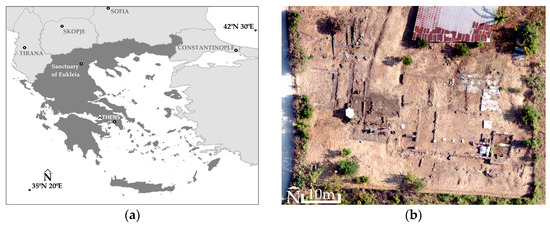
Figure 1.
(a) The location of the archaeological site of the Sanctuary of Eukleia in Greece; (b) The archaeological site of the Sanctuary of Eukleia (excerpt from the orthophotomosaic generated by the RGB images; center of image 40°28′47.56″ N 22°19′16.82″ E).
At this archaeological location, emphasis is placed on the planimetric and vertical accuracy of the LiDAR-derived DSM for both the ruins themselves and the surrounding terrain. In addition, the ability of the LiDAR-derived DTM to survey the adjacent stream banks, located just west of the sanctuary, will also be tested. The stream is cloaked in dense vegetation, shrubs and trees, and its banks exhibit pronounced elevation differences, ranging from approximately 130 m to 155 m (above sea level).
To acquire aerial images the WingtraOne GEN II (Wingtra AG, Zurich, Switzerland), a vertical takeoff and landing (VTOL) fixed-wing UAS, was utilized (Figure 2). It is a fixed-wing aircraft with a maximum take-off weight of 4.8 kg, and a payload capacity of 800 g. Powered by two 99 Wh batteries, it can achieve flight times of up to 59 min at a nominal cruise speed of 16 m/s. The system is designed to operate under sustained winds up to 12 m/s and ambient temperatures ranging from −10 °C to +40 °C, with a maximum take-off altitude of approximately 2500 m above sea level (up to 4800 m when using high-altitude propellers). This has a weight 3.7 kg and measures 125 × 68 × 12 cm. It features an integrated multi-frequency PPK GNSS antenna. Supports multiple satellite systems, including GPS (L1, L2), GLONASS (L1, L2), Galileo (L1), and BeiDou (L1). Flight planning and configuration were performed using the WingtraPilot© software v. 2.18.1. (Wingtra AG, Zurich, Switzerland). The UAS is equipped with both RGB and multispectral (MS) imaging sensors (only one sensor is mounted per flight). The RGB sensor used is the Sony RX1R II (Sony Group Corporation, Tokyo, Japan), a full-frame camera with a 35 mm fixed focal length and a resolution of 42.4 Mp. At a flight altitude of 120 m, it delivers images with a ground sampling distance (GSD) of approximately 1.6 cm per pixel. For multispectral imaging, the system incorporates the MicaSense RedEdge-MX (MicaSense Inc., Seattle, WA, USA). This sensor features a 5.5 mm focal length, 1.2 Mp resolution, and captures data across five spectral bands: blue, green, red, red edge, and near-infrared (NIR). At the same flight altitude of 120 m, it achieves a spatial resolution of 8.2 cm per pixel [13,15].
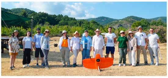
Figure 2.
The Scientific Coordinator of the Summer School Professor D. Kaimaris, the Director of the University Excavation of the Aristotle University of Thessaloniki, Greece, in Aigai (Vergina) Professor A. Kyriakou and the participants of the Summer School ‘’Innovative impression tech-nologies in the service of archaeological excavation and archaeological prospection tools’’ at the archaeological site, after the presentation and the flights carried out by the Scientific Director with the UAS WingtraOne GEN II.
The Topcon HiPer SR GNSS receiver (Topcon Positioning Systems, Tokyo, Japan) was employed [16]. It served two main purposes, first, to collect Check Points (CPs) using real-time kinematic (RTK) positioning, second, to record static GNSS measurements during flight missions (enabling the precise computation of images centers coordinates in the subsequent step). The receiver is compatible with various satellite constellations, including GPS (L1, L2, L2C), GLONASS (L1, L2, L2C), and SBAS-QZSS (L1, L2C). For real-time positioning, the receiver operated in connection with a network of permanent GNSS reference stations (via mobile telecommunication), which provides RTK corrections in real time.
3. Methodology
The methodology includes five main stages (Figure 3):
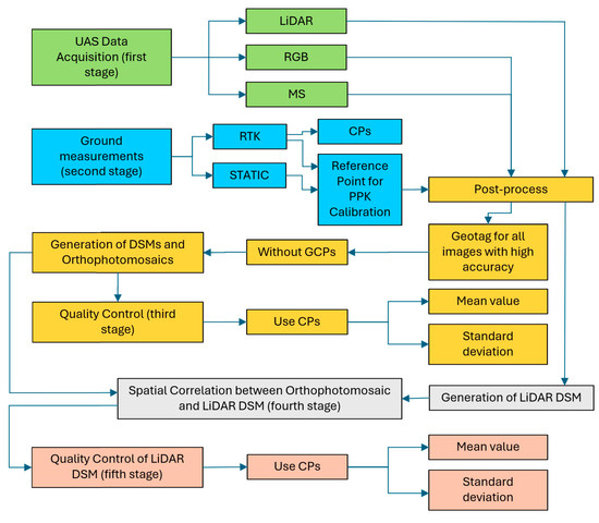
Figure 3.
Stages of Implementation of Methodology.
- Acquisition of RGB, MS images and LiDAR data using UAS over the Sanctuary of Eukleia;
- Collection of ground measurements of 22 CPs with a GNSS receiver. Field measurements with the same receiver also include measuring the reference point for PPK processing;
- Evaluation of the orthophotomosaics by comparing the field-measured coordinates of the 22 CPs with those extracted from the products (orthophotomosaics), calculating the mean values and its standard deviation;
- Assessment of the spatial correlation between the RGB orthophotomosaic and the LiDAR DSM to quantify planimetric offsets or, equivalently, the planimetric accuracy of the LiDAR DSM;
- Comparison of the GNSS-measured elevations of the same 22 CPs with the elevations interpolated from the LiDAR DSM, computing the mean value and standard deviation of the vertical differences.
From these analyses, the overall planimetric and vertical accuracy of the LiDAR DSM is derived.
For product control all established scientific standards were followed, which have been consistently applied in scientific research over the years. Therefore, were used 22 CPs (i.e., more than the minimum required 20) to validate the LiDAR DSM and Photo DSM products. For example, the American Society for Photogrammetry & Remote Sensing (ASPRS) Positional Accuracy Standards [17] explicitly state that accuracy for Non-Vegetated Vertical Accuracy, digital orthoimagery or planimetric data shall not be based on fewer than 20 CPs. Also, the statistical framework adopted here is consistent with the National Standard for Spatial Data Accuracy/Federal Geographic Data Committee (NSSDA/FGDC) methodology [18,19], which has been the reference for accuracy reporting in geospatial products for decades. Assuming random, normally distributed errors with no bias, a sample size of 22 CPs provides a reliable estimate of the root mean square error. The 22 CPs were uniformly distributed across the study area and stratified over the main surface types (archaeological structures and bare ground). None of the CPs were used in the georeferencing or adjustment stage. This sampling strategy increases the representativeness of the checkpoints and reduces the risk of local bias. The new (2023–2024) ASPRS standards [20,21]) and the USGS Lidar Base Specifications recommend a minimum of 30 CPs for new projects large coverage area. However, the present work covers a very small area, and 22 CPs are more than enough. In summary, the 22 CPs constitute a statistically sound and internationally accepted sample size for accuracy evaluation. In this study do not assess ground accuracy under vegetation (west of the archaeological site).
Upon acquiring the Hesai XT32M2X LiDAR (Hesai Technology, Shanghai, China) mounted on the WingtraOne GEN II (Wingtra AG, Zurich, Switzerland), an attempt was made to construct targets (Figure 4) identifiable by their reflectivity in the LiDAR point clouds. Each target has dimensions 70 × 80 cm and contains four internal square frames of 35 × 40 cm, two covered in matte black material and two in white reflective 3M™ Diamond Grade™ Conspicuity Markings Series 983–10 (3M, Saint Paul, MN, USA) [22]. The black panels were expected to absorb most of the laser energy, yielding minimal returns, whereas the white panels should have produced near total reflection and strong returns. Unfortunately, in two preliminary UAS-LiDAR test flights, the targets did not appear in the intensity data. For this reason, the planimetric accuracy assessment of the LiDAR-derived DSM was based not on target detections but on visual correlation with the RGB orthophotomosaic. Future experiments could address this issue by testing alternative reflective materials or by employing commercially available LiDAR-specific calibration targets designed to provide stable and uniform reflectance under varying incidence angles.
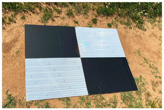
Figure 4.
The target was constructed to assess the three-dimensional accuracy of the LiDAR-derived DSM.
4. Results
4.1. Acquisition of Images and LiDAR Data
All flights were conducted as part of the Summer School “Innovative Impression Technologies in the Service of Archaeological Excavation and Prospection Tools,” held at Aigai (Vergina) from 30 June 2025 to 4 July 2025 (see Acknowledgments). RGB and MS flights were conducted on 1 July 2025 from 9:00 to 10:00 a.m. Mission planning employed a 70% front overlap and 80% side overlap for the RGB sensor (Figure 5a), while the MS sensor utilized 70% overlap in both directions (Figure 5b). The RGB flight was performed at 60 m above-ground level yielding a ground sampling distance (GSD) of approximately 0.8 cm per pixel, and the MS flight at 100 m yielding a GSD of 6.8 cm per pixel. Each flight lasted approximately 4 min, resulting in the capture of 77 RGB and 20 MS images in total. LiDAR data acquisition was conducted on 2 July 2025, from 9:00 to 10:00 a.m., at an altitude of 50 m above ground level and with point density 100 pt/m2 (Figure 5c). The three flight strips provided a 65% overlap between successive point clouds collected. An expanded survey area was delineated, extending southwestward to include LiDAR data acquisition over the stream.
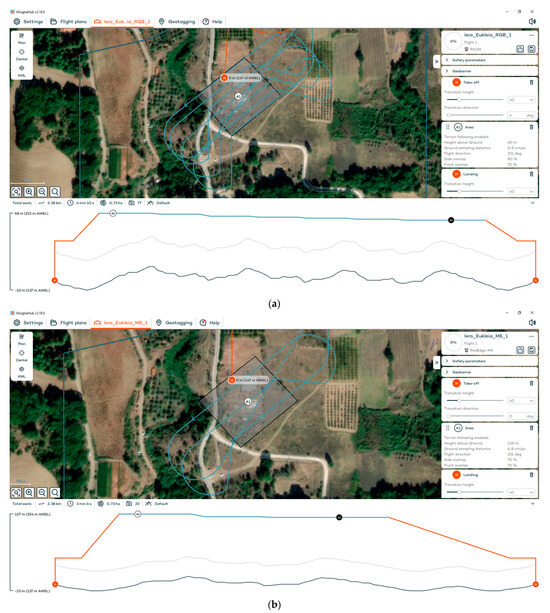
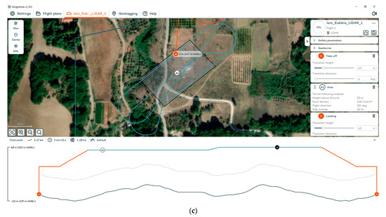
Figure 5.
The flight plan for the (a) RGB sensor; (b) MS sensor; (c) LiDAR. Images from the flight planning software WingtraHub© v2.18.1. (Wingtra AG, Zurich, Switzerland).
4.2. Collection of Check Points and Data Georeferencing
A total of 22 CPs were measured (Figure 6) using a Topcon HiPer SR GNSS receiver (Topcon Positioning Systems, Tokyo, Japan), at the Greek Geodetic Reference System 1987 (GGRS87/Greek Grid, EPSG:2100). Real-time kinematic (RTK) positioning provided a horizontal accuracy of 1.5 cm and a vertical accuracy of 2 cm. Of these, 7 CPs corresponded to readily identifiable corners or internal features of archaeological structures (Figure 6 and Figure 7) and were employed to assess the planimetric and vertical accuracy of the DSMs and orthophotomosaics derived from the RGB and MS images. The remaining 15 CPs are distinct (corners or internal points on the archaeological structures) points or non-distinct (random points on bare ground, Figure 6 and Figure 7) points and used (with other 7 CPs) to evaluate the vertical accuracy of the LiDAR DSM).
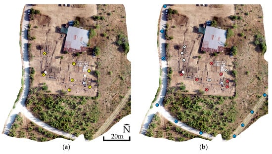
Figure 6.
(a) The 7 CPs (in yellow), out of the total 22, used to validate the RGB and MS orthophotomosaics; (b) The complete set of 22 CPs, where blue denotes random points on bare ground (Figure 7a), white denotes distinct points on the interior surfaces of the archaeological structures (Figure 7b) or at corners of archaeological structures which are at the same level as the ground (Figure 7c), and red denotes corners of the structures elevated above-ground level (Figure 7d); The orthophotomosaic of RGB images in the background; Center of images 40°28′47.59″ N 22°19′16.83″ E.
Figure 7.
(a) With blue arrowed a CP at a random location on bare ground (5 m wide asphalt road, center of image 40°28′46.60″ N 22°19′15.28″ E); (b) With white arrowed a distinct CP on the interior surface of an archaeological structure (0.5 m wide wall; center of image 40°28′48.07″ N 22°19′16.14″ E); (c) With white arrowed a distinct CP at the corner of an archaeological structure (60 × 70 cm; center of image 40°28′47.32″ N 22°19′17.12″ E) that lies flush with the ground; (d) With red arrowed a CP at the corner of an elevated archaeological wall (0.55 m wide; center of image 40°28′47.30″ N 22°19′16.69″ E). The orthophotomosaic of RGB images in the background.
Prior to each flight (RGB, MS, and LiDAR), a randomly selected reference point was established near the UAS home position. Its X, Y, and Z coordinates in GGRS87 (Greek Grid, EPSG:2100) were first determined via RTK with ±1.5 cm horizontal and ±2 cm vertical spatial accuracy. At the same point the receiver then recorded static GNSS observations at that location for 30 min before takeoff, continuously during flight, and for 30 min after landing. By combining the high-precision reference coordinates, static measurements, and in-flight data from the UAS’s integrated multi-frequency PPK GNSS antenna, the projection center positions (X, Y, Z) for each RGB and MS frame were refined during post-processing in WingtraHub© v2.18.1 (Wingtra AG, Zurich, Switzerland), yielding accuracy of 2 cm horizontally and 3 cm vertically (GGRS87/Greek Grid, EPSG:2100).
Using analogous approach, which means using anchored high-accuracy reference point (base), its static observations and LiDAR GNSS/IMU data, the point clouds coordinates were transformed into the geocentric WGS84/UTM Zone 34N system. This transformation and the correlation of overlapping point clouds were performed in the Wingtra LiDAR App© v1.10.1.0. (Wingtra AG, Zurich, Switzerland).
4.3. Generating DSMs, Orthophotomosaics and DTM from Images and UAS-LiDAR
The processing of UAS-derived imagery was conducted using Agisoft Metashape Professional© v2.0.3 (Agisoft LLC, Saint Petersburg, Russia). Upon initiating a project, the images (with high-accuracy center coordinates) set were imported into the software and the coordinate reference system was defined as GGRS87 (Greek Grid, EPSG:2100). For MS datasets, spectral calibration was carried out immediately after import. This step involved capturing calibration targets both prior to and following each flight. These targets were automatically recognized by the software, which then computed reflectance values across all spectral bands [23,24,25,26,27].
Subsequent steps were consistent for both RGB and MS datasets. The images were first oriented based on the precomputed images center coordinates. During this process, the software was set to high accuracy and generic preselection, with key point and tie point limits of 40,000 and 10,000, respectively. During orientation, the projection centers were weighted according to the high-accuracy PPK-derived coordinates, as set automatically by Agisoft Metashape Professional© v2.0.3 (Agisoft LLC, Saint Petersburg, Russia). No additional manual adjustments were applied. The software estimates RMSE values for the camera positions in X, Y, and Z directions (RMSEx, RMSEy, RMSEz), as well as combined values (RMSExy, RMSExyz) to quantify theoretical spatial accuracy [28].
Once images alignment was complete (from RGB or MS sensor), dense point cloud (from RGB or MS images) was generated using high-quality settings (which resample the original image data to one-quarter of their size prior to the matching process) and aggressive depth filtering. This resulted in 55,388,121 points for the RGB dataset and 1,678,461 points for the MS dataset. From these, two 3D mesh models (triangular meshes) were created using the dense cloud as the source (source data: point cloud; surface type: Arbitrary 3D; face count for the RGB: high 15,000,000; face count for the MS: high 440,000; and production of 42,811,371 faces for the RGB and 1,101,396 faces for the MS). Two texture maps were then applied to the meshes using the original imagery (RGB or MS texture type: diffuse map; mapping mode: generic; blending mode: mosaic; texture size: 16,284), thereby producing a visually enhanced 3D models (Table 2). The final products included DSMs and orthophotomosaics.
Table 2.
Data characteristics from RGB, Multispectral (MS) and LiDAR processing workflows.
In the case study of the Sanctuary of Eukleia using RGB imagery, the RMSExyz value of the projection centers was calculated at 1.6 cm. Maximum errors were not directly computed by the software, but the RMSExyz provides a robust estimate of spatial accuracy. The resulting DSM and orthophotomosaic achieved ground resolutions of 1.5 cm and 0.8 cm, respectively (Figure 8). The DSM pixel size was defined based on the density of the dense point cloud, while the orthophotomosaic was generated with a pixel size of corresponding to the native ground sampling distance of the images, to maximize visual detail. For the MS dataset, the RMSExyz was approximately 0.7 cm, with output resolutions of 13.5 cm for the DSM and 7 cm for the orthophotomosaic (Figure 8).
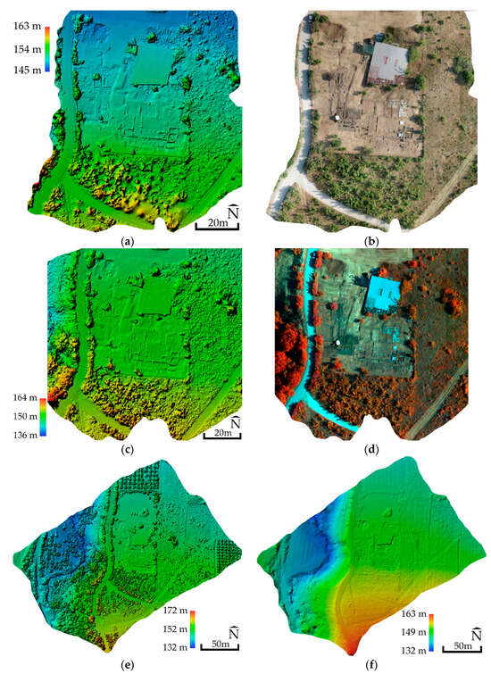
Figure 8.
(a) DSM and (b) orthophotomosaic of the RGB images; (c) DSM and (d) orthophotomosaic (bands NIR-G-B) of the MS images; (e) DSM and (f) DTM from LiDAR; Center of images (a–d) 40°28′47.41″ N 22°19′17.13″ E; (e,f) 40°28′47.59″ N 22°19′16.14″ E.
The correlation of successive UAS-LiDAR point clouds was performed using the Wingtra LiDAR App© v1.10.1.0. (Wingtra AG, Zurich, Switzerland) software, leveraging the high-accuracy reference point (base), its static observations and LiDAR GNSS/IMU data. The flight trajectory was generated using PPK, referenced to base station. According to the two generated reports of the software (Trajectory Generator Report and Point Cloud Generation Report) the GNSS solution maintained predominantly fixed ambiguity resolution in both forward and reverse processing, instances of single or no direction fixes were negligible, indicating high-quality positioning. The discrepancy between forward and reverse trajectories remained minimal, further confirming precise trajectory tracking and stable flight performance. To generate the final point cloud, angular scan and range filters (315–45° scan angle; 8–200 m range) were applied to exclude low-reliability returns. The resulting cloud was referenced in the WGS84/UTM Zone 34 N coordinate system. Although the software does not include quantitative tools for assessing strip-to-strip alignment, the high-quality trajectory data and the system’s built-in calibration ensure that strip registration falls within typical tolerances for high-precision applications.
The final LAS file was exported from the Wingtra LiDAR App© v.1.10.1.0. (Wingtra AG, Zurich, Switzerland) was imported into Agisoft Metashape Professional© v2.0.3 (Agisoft LLC, Saint Petersburg, Russia). Point cloud coordinates were converted from the geocentric system to GGRS87 (Greek Grid, EPSG:2100), and automatic ground-point classification was performed with the following settings: Max angle 45° (the maximum slope between the temporary ground model and the line connecting a candidate point to an already classified ground point), max distance 0.05 m (the maximum vertical distance of a point from the temporary ground model), max terrain slope 45° (the steepest natural terrain slope allowed), cell size 5 m (the side length of the grid cells used to pick the lowest point in each cell for the initial ground model), and erosion radius 0 m (the buffer around each point within which points with large elevation differences are removed). This workflow produced two LAS files, the DSM and the DTM of the study area (Figure 8), with an average point spacing of approximately 10 cm, resulting from a flight height of 50 m.
4.4. Evaluation of the Horizontal and Vertical Accuracy of the LiDAR-Derived DSM
To assess the planimetric and vertical accuracy of the LiDAR DSM, the RGB-based DSM and orthophotomosaic were first evaluated using 7 distinct CPs (corners or interior features of the archaeological structures; Figure 6a), even though the manufacturer recommends just 3 CPs [18]. Planimetric differences were minimal, with a mean of 1.4 cm (with standard deviation σ = ±1 cm) in X and 0.9 cm (with σ = ±0.9 cm) in Y. These results are fully consistent with previous studies [29,30] and agree with the accuracy specifications provided by the UAS manufacturer [18]. A similar assessment of the MS derived products yielded mean planimetric offsets of 3 cm (with σ = ±2 cm) in X and 2 cm (with σ = ±1 cm) in Y.
Given the exceptional planimetric precision of the RGB products, the RGB orthophotomosaic was chosen as the “reference base” for further comparative analyses. Specifically, examined whether the LiDAR DSM is spatially aligned with the RGB orthophotomosaic (Figure 9).
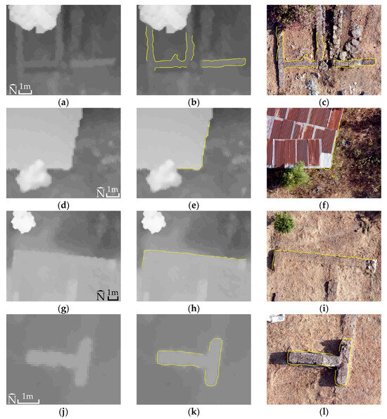
Figure 9.
(a,d,g,j) The LiDAR-derived DSM is shown in grayscale (white tones for higher elevations, dark tones for lower elevations; (a,d): 149–152 m; (g): 149–154 m; (j): 151–152 m); (b,e,h,k) The construction boundaries are delineated in yellow on the DSM; and (c,f,i,l) those boundaries are overlaid on the RGB orthophotomosaic to assess their spatial correspondence. Center of images (a–c) 40°28′48.07″ Ν 22°19′16.14″ E; Center of images (d–f) 40°28′48.15″ Ν 22°19′17.63″ E; (g–i) 40°28′47.81″ N 22°19′16.99″ E; (j–l) 40°28′47.34″ N 22°19′16.86″ E.
The visual comparison (Figure 9) demonstrated that the two products are positionally coincided, with only minor, non-systematic, randomly offsets in a few instances. Therefore, it is accepted that both deliver approximately the same planimetric accuracy. Consequently, all 22 CPs (Figure 6) were projected directly onto the LiDAR DSM, without any horizontal adjustments, to assess its vertical accuracy. For each CP (i = 1…22), measured by GNSS with RTK, the elevation difference ΔZi = Zi − Zi’ was computed (where Zi is the GNSS measured elevation and Zi’ is the DSM elevation). These calculations revealed a mean vertical difference of 7.5 cm (σ = ±6 cm, Equation (1) with N = 22), representing the LiDAR DSM’s vertical accuracy over the study area (Table 3).
Table 3.
Vertical accuracy results of LiDAR DSM product.
Notably, the largest vertical discrepancies occurred at the 7 CPs located at elevated corners of archaeological structures (red arrowed in Figure 6b and Figure 7d), which yielded a mean ΔZ of 13 cm (with σ = ±6.5 cm). In contrast, the remaining 15 CPs, random points on bare ground and distinct points on interior surfaces or ground level corners of the structures (blue and white arrowed in Figure 6b and Figure 7a–c) exhibited a mean ΔZ of 5 cm (with σ = ±3 cm).
Regarding the streambanks adjacent to the archaeological site, LiDAR successfully captured their topography to a satisfactory degree (Figure 10).
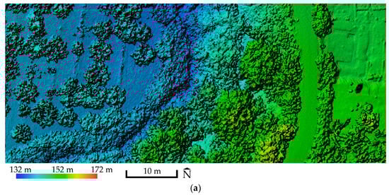
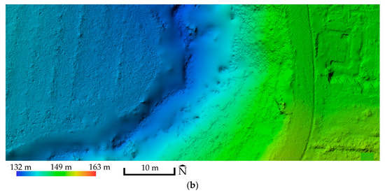
Figure 10.
(a) Excerpt of the LiDAR-derived DSM; (b) and the LiDAR-derived DTM; Center of images 40°28′47.28″ N 22°19′13.70″ E.
5. Discussion
The exceptionally good RMSExyz values, 1.6 cm for RGB and 0.7 cm for MS images, demonstrate, on the one hand, the theoretically high accuracy of the DSMs and orthophotomosaics which will arise and, on the other, underscore the benefits of using PPK technology without GCPs in image processing. In practice, product evaluations (Figure 6a) returned equally good planimetric accuracies of 1.4 cm (with σ = ±1 cm) in X and 0.9 cm (with σ = ±0.9 cm) in Y for the RGB images, and 3 cm (with σ = ±2 cm) in X and 2 cm (with σ = ±1 cm) in Y for the MS images.
A LiDAR point density of 100 pt/m2 at a 50 m flight height ensures fine detail capture of both terrain and built features. The absence of built-in software tools to verify point cloud alignment introduces an uncertainty that can only be resolved through direct evaluation of the final DSM product.
The visual comparison approach (LiDAR-derived DSM with RGB orthophotomosaic) carries an inherent risk of misinterpretation, but examination of Figure 9 imagery (and more sites) supports the conclusion that the LiDAR-derived DSM’s planimetric accuracy closely matches that of the RGB orthophotomosaic. So, given a planimetric accuracy of, approximately, 1.4 cm (with σ = ±1 cm) in X and 0.9 cm (with σ = ±0.9 cm) in Y for the LiDAR DSM, all 22 CPs were projected directly onto the DSM. Vertical discrepancies ΔZi = Zi − Zi’ (Zi from CPi,GNSS, Zi’ from CPi,DSM and i = 1–22, Figure 6b) yielded a mean vertical difference of 7.5 cm with σ = ±5.5 cm.
The largest vertical errors originated from CPs located at the corners of archaeological structures, elevated features relative to the ground (Figure 6b and Figure 7d), because the interpolated DSM heights there combine returns from ground-level points and returns from the higher structural surfaces. When isolating only those corner CPs, the mean vertical error worsened to 13 cm (with σ = ±6.5 cm).
By contrast, CPs positioned either on bare ground, within the interior surfaces of structures, or at corners flush with the ground plane (Figure 6b and Figure 7a–c) exhibited excellent vertical accuracy. For these points, the mean vertical error was just 5 cm with σ = ±3 cm, due to the interference of points that are on the same elevation level.
A comparable vertical assessment of the DSM from RGB images derived using all 22 CPs (Figure 6b) produced a mean vertical difference of 2.4 cm (with σ = ±1.7 cm). Thus, in this study, PPK-processed RGB imagery (without GCPs) yielded superior vertical accuracy compared to the LiDAR-based DSM.
To place the accuracy results of this study in context, it is useful to compare them with findings from some UAV-LiDAR surveys in both cultural heritage and other domains such as critical infrastructure and environmental monitoring. UAV-LiDAR systems have demonstrated the ability to capture high-density 3D point clouds with high-level precision, provided that data quality is carefully assessed and controlled [31]. For instance, evaluations of heterogeneous vegetation types showed horizontal accuracies around 0.05 m and vertical accuracies up to 0.24 m, with variations among vegetation types highlighting the influence of canopy structure on measurement errors [32]. Environmental studies further illustrate the sensitivity of UAV-LiDAR accuracy to survey parameters. In coastal marshes, higher flight altitudes generally improved ground penetration and reduced vertical errors, while oblique scan angles produced higher RMSE values compared to nadir scans [33,34]. Similarly, surveys over complex forested or vegetated terrains indicated that dense canopy could increase vertical RMSE to ~0.21 m, whereas open areas achieved RMSE as low as 0.07 m, emphasizing the importance of flight planning and ground control distribution [35]. Studies on UAV-LiDAR for infrastructure and high-precision applications also highlight the effect of baseline setup, scanner warm-up, and environmental conditions on both horizontal and vertical accuracy [36]. In cultural heritage contexts, UAV-LiDAR has proven effective for detecting fine-scale topographic features beneath vegetation and other obstructions. For example, UAV-LiDAR surveys have successfully captured microtopographic details of archaeological sites under leafy cover with vertical accuracies around 0.12 m [31]. Comparable results have been achieved in diverse and challenging environments, including forested, mountainous, and erosion-prone regions, where UAV-LiDAR and photogrammetry have been jointly applied to detect and interpret archaeological features hidden beneath dense canopy. Recent studies demonstrate its exceptional capability to reveal complex ritual and habitation landscapes under forest cover in the Greater Khingan Range of northeastern China [37], to monitor ongoing excavations through precise 3D recording of stratigraphy and terrain deformation [38], and to identify lost medieval settlements in hilly Mediterranean areas through advanced filtering and semi-automatic feature extraction [39]. Comparisons of UAV-LiDAR with Structure-from-Motion photogrammetry in similar archaeological and riverine settings have shown comparable vertical precision (with vertical accuracy around 0.12 m), confirming the reliability of UAV-LiDAR for documenting subtle terrain variations critical for cultural heritage studies [40].
The term Precision Archaeology could refer to the use of modern, innovative technologies for the acquisition, processing and analysis of high-spatial-resolution data aimed at decision-making for the conservation, restoration and protection of our Cultural Heritage. The state-of-the-art equipment employed in this paper and the 3D spatial accuracy of the products from RGB and MS images processing satisfy the requirements of Precision Archaeology. About UAS-LiDAR, at present and for the sole application in this study, only the planimetric accuracy of its output aligns with the concept of Precision Archaeology. A key advantage of UAS-LiDAR is its ability to penetrate vegetation and capture ground detail beneath tree canopies, something not possible with RGB images. With a point density of 100 pt/m2 at a 50 m flight height, UAS-LiDAR successfully mapped the adjacent streambank almost in its entirety. So, it could, perhaps, capture above-ground archaeological remains covered by natural vegetation.
6. Conclusions
Regarding the paper’s objectives, the LiDAR-derived DSM exhibited outstanding planimetric accuracy, on the order of 1.4 cm (with σ = ±1 cm) in X and 0.9 cm (with σ = ±0.9 cm) in Y. Its vertical accuracy was also very good, 7.5 cm (with σ = ±5.5 cm) over mixed surfaces, i.e., areas combining moderate relief (such as smooth ground) and pronounced relief (such as terrain plus built structures). Particularly noteworthy is the vertical accuracy on smoothly varying terrain, which reached 5 cm (with σ = ±3 cm). Of course, these results pertain to a single test site, so further evaluations across multiple areas are needed to draw more robust conclusions about the DSM’s 3D spatial accuracy.
Better vertical accuracy might be achieved by designing perpendicular flight strips within the same mission to capture LiDAR data from cross flights. This hypothesis should be tested in upcoming applications.
In this study, the vertical accuracy obtained from the RGB imagery alone (using PPK technology without GCPs) surpassed that of the LiDAR data. However, it is important to note that the LiDAR data have an average point spacing of roughly 10 cm at a 50 m flight height, whereas the RGB imagery from a comparable flight height (60 m) achieves a ground sampling distance (GSD) of about 0.8 cm. Although the LiDAR vertical accuracy is numerically low, its dense point spacing (~10 cm) and ability to capture fine-scale topographic details, including areas beneath trees and shrubs, provide a level of spatial detail and completeness that cannot be matched by high-altitude aerial surveys. Therefore, despite the similar order of magnitude of vertical accuracy with high-altitude aerial surveys, UAS LiDAR remains highly valuable for mapping complex archaeological and natural terrains.
Commercial integration of LiDAR on UAS began around 10 years ago, so there remains room for advances in both point density and overall spatial accuracy of the products.
It is encouraging that LiDAR successfully captured ground beneath trees and shrubs during flowering (July), effectively mapping almost the entire streambank topography. Collecting data in the winter months could further increase ground-capture rates. This under vegetation mapping capability is crucial, as there are plans to use this LiDAR system in future aerial remote sensing archaeology [41] studies, to locate unknown above-ground archaeological remains concealed beneath natural vegetation, in areas resulting from the study of the bibliography.
Funding
This research received no external funding.
Data Availability Statement
No original images or raw data will be made available on the locations, as they concern archaeological site.
Acknowledgments
The data presented in this paper, namely CPs, LiDAR data, RGB and MS images, were collected by Dimitri Kaimari, Scientific Coordinator of the Summer School “Innovative Impression Technologies in the Service of Archaeological Excavation and Archaeological Prospection Tools” held at Aigai (Vergina, Central Macedonia, Greece) from 30 June to 4 July 2025, through receiver GNSS and flights conducted using the UAS WingtraOne GEN II. Sincere thanks are extended to A. Kyriakou, key collaborator of the Summer School and Director of the University Excavation of the Aristotle University of Thessaloniki, Greece, in Aigai, for our excellent cooperation and for granting permission for the data collection at the archaeological site of the Sanctuary of Eukleia. Also, warm thanks to all participants who followed the data acquisition processes and coursework with outstanding engagement, forming a unique interdisciplinary team of high scientific caliber.
Conflicts of Interest
The author declares no conflicts of interest.
References
- Kovanič, Ľ.; Topitzer, B.; Peťovský, P.; Blišťan, P.; Gergeľová, M.B.; Blišťanová, M. Review of Photogrammetric and Lidar Applications of UAV. Appl. Sci. 2023, 13, 6732. [Google Scholar] [CrossRef]
- Seidaliyeva, U.; Ilipbayeva, L.; Utebayeva, D.; Smailov, N.; Matson, E.T.; Tashtay, Y.; Turumbetov, M.; Sabibolda, A. LiDAR Technology for UAV Detection: From Fundamentals and Operational Principles to Advanced Detection and Classification Techniques. Sensors 2025, 25, 2757. [Google Scholar] [CrossRef]
- Walker, M.; Dahle, A.G. Literature Review of Unmanned Aerial Systems and LIDAR with Application to Distribution Utility Vegetation Management. Arboric. Urban For. 2023, 49, 144–156. [Google Scholar] [CrossRef]
- Bartmiński, P.; Siłuch, M.; Kociuba, W. The Effectiveness of a UAV-Based LiDAR Survey to Develop Digital Terrain Models and Topographic Texture Analyses. Sensors 2023, 23, 6415. [Google Scholar] [CrossRef]
- Adamopoulos, E.; Rinaudo, F. UAS-Based Archaeological Remote Sensing: Review, Meta-Analysis and State-of-the-Art. Drones 2020, 4, 46. [Google Scholar] [CrossRef]
- Bouziani, M.; Amraoui, M.; Kellouch, S. Comparison Assessment of Digital 3D Models Obtained by Drone-Based LiDAR and Drone Imagery. Int. Arch. Photogramm. Remote Sens. Spat. Inf. Sci. 2021, XLVI-4/W5-2021, 113–118. [Google Scholar] [CrossRef]
- Sudra, P.; Demarchi, L.; Wierzbicki, G.; Chormański, J. A Comparative Assessment of Multi-Source Generation of Digital Elevation Models for Fluvial Landscapes Characterization and Monitoring. Remote Sens. 2023, 15, 1949. [Google Scholar] [CrossRef]
- Sestras, P.; Badea, G.; Badea, C.A.; Salagean, T.; Roșca, S.; Kader, S.; Remondino, F. Land surveying with UAV photogrammetry and LiDAR for optimal building planning. Autom. Constr. 2025, 173, 106092. [Google Scholar] [CrossRef]
- Oniga, V.-E.; Loghin, A.-M.; Macovei, M.; Lazar, A.-A.; Boroianu, B.; Sestras, P. Enhancing LiDAR-UAS Derived Digital Terrain Models with Hierarchic Robust and Volume-Based Filtering Approaches for Precision Topographic Mapping. Remote Sens. 2024, 16, 78. [Google Scholar] [CrossRef]
- Mandlburger, G.; Kolle, M.; Poppl, F.; Cramer, M. Evaluation of Consumer-Grade and Surve-Grade UAV-LiDAR. Int. Arch. Photogramm. Remote Sens. Spat. Inf. Sci. 2023, XLVIII-1/W3-2023, 99–106. [Google Scholar] [CrossRef]
- Chaudhry, M.H.; Ahmad, A.; Gulzar, Q.; Farid, M.S.; Shahabi, H.; Al-Ansari, N. Assessment of DSM Based on Radiometric Transformation of UAV Data. Sensors 2021, 21, 1649. [Google Scholar] [CrossRef]
- Van Alphen, R.; Rains, K.C.; Rodgers, M.; Malservisi, R.; Dixon, T.H. UAV-Based Wetland Monitoring: Multispectral and Lidar Fusion with Random Forest Classification. Drones 2024, 8, 113. [Google Scholar] [CrossRef]
- WingtraOne GEN II, Technical Specifications. Available online: https://wingtra.com/wp-content/uploads/Wingtra-Technical-Specifications.pdf (accessed on 16 July 2025).
- Kyriakou, A. The sanctuary of Eukleia at Vergina-Aegae: Aspects of the development of a cult place in the heart of the Macedonian Kingdom. In Proceedings of the Ancient Macedonia: The Birth of Hellenism at the Origins of Europe, Università La Sapienza, Facoltà di Lettere e Filosofia Aula Odeion (Museo dell’Arte Classica), Roma, Italy, 14–15 December 2017. [Google Scholar]
- RedEdge-MX Integration Guide. Available online: https://support.micasense.com/hc/en-us/articles/360011389334-RedEdge-MX-Integration-Guide (accessed on 16 July 2025).
- HiPer SR. Available online: https://mytopcon.topconpositioning.com/support/products/hiper-sr (accessed on 16 July 2025).
- American Society for Photogrammetry and Remote Sensing. ASPRS Positional Accuracy Standards for Digital Geospatial Data, Edition 1, Version 1.0, November 2014. Photogramm. Eng. Remote Sens. 2015, 81, A1–A26. [Google Scholar]
- Minnesota Geospatial Information Office. Positional Accuracy Handbook (NSSDA); Minnesota Geospatial Information Office: St. Paul, MN, USA, 1999; Available online: https://www.mngeo.state.mn.us/committee/standards/positional_accuracy/positional_accuracy_handbook_nssda.pdf (accessed on 21 September 2025).
- FGDC-STD-007.3-1998; Geospatial Positioning Accuracy Standards Part 3: National Standard for Spatial Data Accuracy. Federal Geographic Data Committee: Washington, DC, USA, 1998. Available online: https://www.fgdc.gov/standards/projects/accuracy/part3/chapter3 (accessed on 21 September 2025).
- U.S. Geological Survey. Lidar Base Specification: Revision History; National Geospatial Program; U.S. Geological Survey: Reston, VA, USA, 2025. Available online: https://www.usgs.gov/ngp-standards-and-specifications/lidar-base-specification-revision-history (accessed on 21 September 2025).
- Abdullah, Q. ASPRS Positional Accuracy Standards, Edition 2: The Geospatial Mapping Industry Guide to Best Practices. Photogramm. Eng. Remote Sens. 2023, 89, 581–588. [Google Scholar] [CrossRef]
- 3M™ Diamond Grade™ Conspicuity Markings Series 983 for Trucks and Trailers. Available online: https://multimedia.3m.com/mws/media/1241053O/pb-983-truck-trail-fm.pdf (accessed on 16 July 2025).
- Franzini, M.; Ronchetti, G.; Sona, G.; Casella, V. Geometric and radiometric consistency of parrot sequoia multispectral imagery for precision agriculture applications. Appl. Sci. 2019, 9, 5314. [Google Scholar] [CrossRef]
- Guo, Y.; Senthilnath, J.; Wu, W.; Zhang, X.; Zeng, Z.; Huang, H. Radiometric calibration for multispectral camera of different imaging conditions mounted on a UAS platform. Sustainability 2019, 11, 978. [Google Scholar] [CrossRef]
- Assmann, J.J.; Kerby, T.J.; Cunliffe, M.A.; Myers-Smith, H.I. Vegetation monitoring using multispectral sensors best practices and lessons learned from high latitudes. J. Unmanned Veh. Syst. 2019, 7, 54–75. [Google Scholar] [CrossRef]
- Windle, A.E.; Silsbe, G.M. Evaluation of Unoccupied Aircraft System (UAS) Remote Sensing Reflectance Retrievals for Water Quality Monitoring in Coastal Waters. Front. Environ. Sci. 2021, 9, 674247. [Google Scholar] [CrossRef]
- Daniels, L.; Eeckhout, E.; Wieme, J.; Dejaegher, Y.; Audenaert, K.; Maes, W.H. Identifying the Optimal Radiometric Calibration Method for UAV-Based Multispectral Imaging. Remote Sens. 2023, 15, 2909. [Google Scholar] [CrossRef]
- Agisoft Metashape User Manual, Professional Edition, Version 2.0. Available online: https://www.agisoft.com/pdf/metashape-pro_2_0_en.pdf (accessed on 16 July 2025).
- Kaimaris, D. Measurement Accuracy and Improvement of Thematic Information from Unmanned Aerial System Sensor Products in Cultural Heritage Applications. Imaging 2024, 10, 34. [Google Scholar] [CrossRef]
- Kaimaris, D.; Kalyva, D. Aerial Remote Sensing and Urban Planning Study of Ancient Hippodamian System. Urban Sci. 2025, 9, 183. [Google Scholar] [CrossRef]
- Elaksher, A.; Ali, T.; Alharthy, A. A Quantitative Assessment of LIDAR Data Accuracy. Remote Sens. 2023, 15, 442. [Google Scholar] [CrossRef]
- Kucharczyk, M.; Hugenholtz, H.C.; Zou, X. UAV–LiDAR accuracy in vegetated terrain. J. Unmanned Veh. Syst. 2018, 6, 212–234. [Google Scholar] [CrossRef]
- Amelunke, M. Influence of Altitude and Scan Angle on UAS-LiDAR Ground Height Measurement Accuracy in Juncus roemerianus Scheele (Black Needle Rush)-Dominated Marshes. Master’s Thesis, Master of Biological Environmental and Earth Sciences, University of Southern Mississippi, Hattiesburg, MS, USA, 14 May 2022. [Google Scholar]
- Curcio, C.A.; Peralta, G.; Aranda, M.; Barbero, L. Evaluating the Performance of High Spatial Resolution UAV-Photogrammetry and UAV-LiDAR for Salt Marshes: The Cádiz Bay Study Case. Remote Sens. 2022, 14, 3582. [Google Scholar] [CrossRef]
- Tamimi, R.; Toth, C. Accuracy Assessment of UAV LiDAR Compared to Traditional Total Station for Geospatial Data Collection in Land Surveying Contexts. Int. Arch. Photogramm. Remote Sens. Spat. Inf. Sci. 2024, XLVIII-2-2024, 421–426. [Google Scholar] [CrossRef]
- Lassiter, H.A.; Wilkinson, B.; Gonzalez Perez, A.; Kelly, C. Absolute 3D Accuracy Assessment of UAS LiDAR Surveying. Int. Arch. Photogramm. Remote Sens. Spat. Inf. Sci. 2021, XLIV-M-3-2021, 105–111. [Google Scholar] [CrossRef]
- Li, Z. New opportunities for archaeological research in the Greater Ghingan Range, China: Application of UAV LiDAR in the archaeological survey of the Shenshan Mountain. J. Archaeol. Sci. Rep. 2023, 51, 104182. [Google Scholar] [CrossRef]
- Adamopoulos, E.; Papadopoulou, E.E.; Mpia, M.; Deligianni, O.E.; Papadopoulou, G.; Athanasoulis, D.; Konioti, M.; Koutsoumpou, M.; Anagnostopoulos, N.C. 3D Survey and Monitoring of Ongoing Archaeological Excavations Via Terrestrial and Drone LiDAR. ISPRS Ann. Photogramm. Remote Sens. Spat. Inf. Sci. 2023, X-M-1-2023, 3–10. [Google Scholar] [CrossRef]
- Masini, N.; Abate, N.; Gizzi, F.T.; Vitale, V.; Minervino Amodio, A.; Sileo, M.; Biscione, M.; Lasaponara, R.; Bentivenga, M.; Cavalcante, F. UAV LiDAR Based Approach for the Detection and Interpretation of Archaeological Micro Topography under Canopy—The Rediscovery of Perticara (Basilicata, Italy). Remote Sens. 2022, 14, 6074. [Google Scholar] [CrossRef]
- Muller, A. Assessment of Vertical Accuracy from UAV-LiDAR and Structure from Motion Point Clouds in Floodplain Terrain Mapping. Master’s Thesis, Master of Science in Geography, Portland State University, Portland, OR, USA, 29 December 2021. [Google Scholar]
- Kaimaris, D. Aerial Remote Sensing Archaeology—A Short Review and Applications. Land 2024, 13, 997. [Google Scholar] [CrossRef]
Disclaimer/Publisher’s Note: The statements, opinions and data contained in all publications are solely those of the individual author(s) and contributor(s) and not of MDPI and/or the editor(s). MDPI and/or the editor(s) disclaim responsibility for any injury to people or property resulting from any ideas, methods, instructions or products referred to in the content. |
© 2025 by the author. Licensee MDPI, Basel, Switzerland. This article is an open access article distributed under the terms and conditions of the Creative Commons Attribution (CC BY) license (https://creativecommons.org/licenses/by/4.0/).