A Geostatistical Predictive Framework for 3D Lithological Modeling of Heterogeneous Subsurface Systems Using Empirical Bayesian Kriging 3D (EBK3D) and GIS

Abstract

Predicting subsoil properties accurately is important for engineering tasks like construction, land development, and environmental management. However, traditional approaches that use borehole data often face challenges because the data is sparse and unevenly spread, which can cause uncertainty in understanding the subsurface. This study introduces a novel geostatistical framework employing Empirical Bayesian Kriging 3D (EBK3D) within a Geographic Information System (GIS), which was developed to construct three-dimensional lithological models. The framework was applied to 265 boreholes from the Queen Mary Reservoir in London. ArcGIS Pro was used to interpolate lithology layers using EBK3D, resulting in voxel-based models that represent both horizontal and vertical lithological variations. Model validation was performed with an independent dataset comprising 30% of the boreholes. The results demonstrated high predictive accuracy for layer elevations (Pearson’s r = 0.99, MAE = 0.31 m). The model achieved 100% accuracy in predicting borehole stratigraphy in homogenous zones and correctly identified 77% of lithological layers in heterogeneous zones. In complex regions, the model accurately predicted the whole borehole in 49% of cases. This framework provides a reliable, repeatable, and cost-effective method for three-dimensional subsurface characterization, enhancing traditional approaches by automating uncertainty quantification and capturing both vertical and horizontal variability.

1. Introduction

Subsurface conditions are an important parameter in the analysis and design of geotechnical structures and facilities. The nature and variety of the soil profile and its properties play a significant role in determining geotechnical design parameters for the design and construction of underground utilities and foundations [1]. Also, the most important step in urban planning and risk assessment is to identify the subsurface data of the urban area [2].

The subsurface data can be gathered through traditional drilling techniques, modern geophysical techniques, or integration of both [1]. The borehole data acquired from drilling operations are managed using boring coordinates, ground level, geological data by depth, and site test results. The coordinates of boreholes indicate a horizontal location, and with the aid of the relative height between depth and ground level, it is possible to determine the vertical position of the borehole location. Therefore, boreholes are the most significant data source for 3D geological modeling [3]. The processed borehole data become 3D spatial data that can be used to browse geological data by depth. Such georeferenced borehole data can be applied in diverse spatial modeling, such as geology modeling [4], groundwater table distribution estimation [5], and assessment of seismic liquefaction [6]. However, since individual boreholes consist of 3D coordinates, general 2D interpolation techniques are limited in fully capturing the nature of borehole data that are densely distributed vertically along the ground surface [7].

As boreholes provide information about the subsoil only at a limited number of points, interpolation needs to be carried out between the investigated points to predict unsampled locations. Hence, spatial interpolation techniques develop spatially continuous data sets from the sparsely distributed punctual data. Various interpolation techniques exist, e.g., deterministic and geostatistical [8]. The precision of the interpolated outcomes relies on the quantity and distribution of the data points utilized for calculation [9]. Deterministic interpolation methods, such as Inverse Distance Weighting (IDW) and radial basis functions (RBFs), are restricted in their capacity for fitting complex spatial variation as well as quantifying uncertainty in predictions [7,10]. Empirical Bayesian Kriging (EBK), a geostatistical approach that uses Bayesian inference in conjunction with kriging, addresses many of these limitations by automatically fitting model parameters and giving more precise predictions.

In contrast to classic kriging techniques, which rely on manual parameterization, EBK uses automatic parameterization based on subsetting and simulation. Because of this characteristic, EBK is especially helpful in addressing complex spatial variability and prediction uncertainty [11,12,13]. Numerous studies have demonstrated that using EBK for subsurface modeling produces predictions that are more accurate than those made using conventional methods. EBK3D’s ability to handle complex spatial variability is demonstrated by its successful use in interpolating groundwater quality and soil contamination concentrations [12,13]. Nevertheless, there are no studies on the creation of a 3D subsurface using EBK3D and borehole data.

A Geographic Information System (GIS) is crucial for conducting spatial regression analysis to objectively measure and correlate urban metrics with social data, identifying key patterns and relationships [14,15]. Additionally, it offers a vital platform for combining, organizing, and evaluating various high-resolution spatial datasets into a single processing framework, such as LiDAR data and climate model outputs [16]. This is essential for guiding urban development plans [17] and sustainable urban planning [18].

The creation of 3D subsurface models was greatly enhanced by the combination of GIS and geostatistical methods. While geostatistical techniques allow sparse data to be interpolated into continuous 3D models, GIS provides a framework for managing, analyzing, and visualizing spatial data [19,20]. Recent research has illustrated the utility of GIS-based 3D modeling in a range of applications such as urban geology [21], landslide risk mapping [22], and hydrocarbon exploration [20]. One challenge in 3D subsurface modeling is the precise prediction of vertical variability in layered geological formations [23,24,25].

Although several studies have demonstrated the robustness of EBK and its three-dimensional variant (EBK3D) in applications such as groundwater quality mapping, soil contamination assessment, and environmental modeling [12,13,26,27,28,29], their direct use for borehole-based lithological modeling remains very limited. The research gap lies in the absence of studies that integrate EBK3D with borehole datasets to capture both horizontal and vertical variability in subsurface materials. Most existing work on generating 3D subsurface models uses digital elevation model (DEM) stacking [1] or interpolation at equal vertical intervals, which have advanced subsurface visualization but present critical shortcomings [13,25]. Moreover, previous studies rarely combine EBK3D within a GIS environment to create voxel-based 3D subsurface models. This study addresses that research gap by developing a GIS-based predictive framework that applies EBK3D to borehole data for accurate and uncertainty-aware 3D lithological modeling in heterogeneous geological systems.

The novelty of this work lies in the following factors:

• This study presents the first application of EBK3D for three-dimensional lithological modeling from borehole data within a fully integrated geographic information system (GIS) workflow.
• The research introduces a reproducible methodology that converts sparse borehole logs into a continuous one-dimensional Model of Borehole Data (1DMGD), thereby enhancing the reliability of voxel-based interpolation.

The study offers a comprehensive validation that measures performance on the more difficult task of predicting entire stratigraphic sequences in both homogeneous and heterogeneous geological environments, as well as layer depth estimation.

The following briefly describes this paper’s contribution:

• In a GIS environment, we create an effective geostatistical predictive framework that uses borehole data to directly predict 3D subsurface stratigraphy. This is accomplished by successfully integrating EBK3D with GIS.
• Enhancing traditional interpolation techniques by using EBK3D to quantify uncertainty and capture spatial autocorrelation.
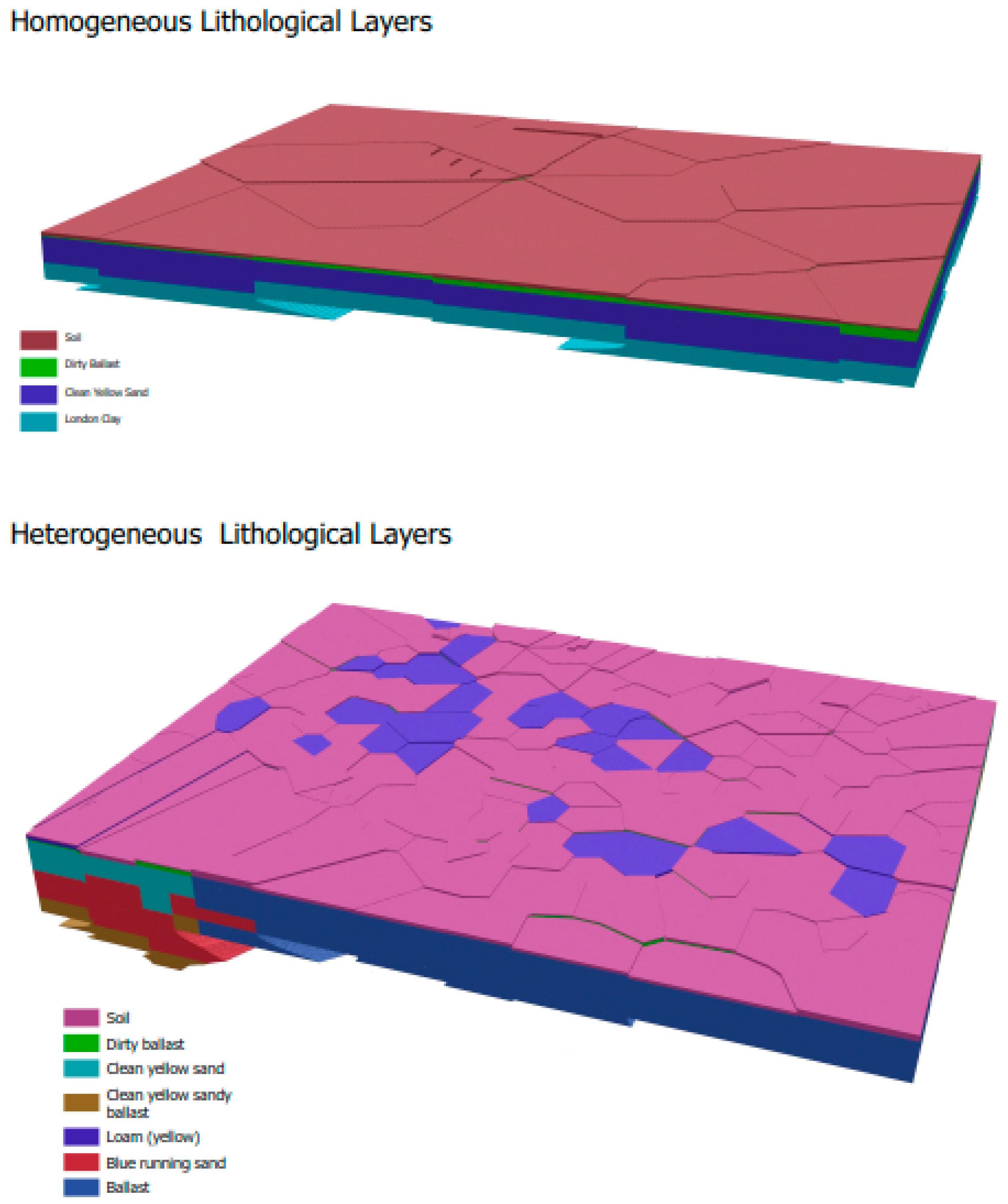
• To test the suggested framework’s adaptability and resilience, we compare it in heterogeneous and homogeneous geological scenarios.
• Providing accurate volumetric subsurface representations to aid in engineering, environmental, and geotechnical decision-making.

This paper is structured as follows: Section 2 introduces a literature review regarding the paper’s subject, including Subsurface Modeling, Traditional Methods for Subsurface Modeling, and lastly Advances in 3D Subsurface Modeling. Section 3 presents the proposed methodology of 3D Lithological Modeling of Heterogeneous Subsurface Systems using EBK3D and GIS. The results analysis and discussion are presented in Section 4, while the research limitations of this study are explored in Section 5. Finally, Section 6 concludes the paper by summarizing key insights in this innovative topic.

2. Literature Review

This section presents the paper’s key topics, which include subsurface modeling, traditional methods, recent advances in three-dimensional subsurface modeling, and the application of EBK3D as the primary approach in this study.

2.1. Subsurface Modeling

Subsurface modeling is essential process in geotechnical engineering, urban planning, and environmental management. Accurate characterization of subsurface lithology and properties supports effective infrastructure design, risk assessment, and resource management [1,2]. Nonetheless, conventional techniques rely on frequently sparse and unevenly distributed borehole data, which introduces uncertainty into subsurface characterization [3]. Interpolating these discrete data points into continuous 3D models that faithfully capture subsurface heterogeneity is the primary challenge.

2.2. Traditional Methods for Subsurface Modeling

The traditional methods for subsurface modeling can be summarized as follows:

▪

Deterministic Interpolation Methods: Techniques for Deterministic Interpolation: Spatial interpolation frequently uses deterministic techniques such as Radial Basis Functions (RBFs) and Inverse Distance Weighting (IDW). These approaches are straightforward, but they typically overlook intricate spatial variability and uncertainty [10].

▪

Geostatistical Interpolation Methods: The geostatistics approach examines a parameter’s spatial pattern across sampled locations. Using this data, a statistical model is developed that takes into account the distance between unsampled points and predicts the value of the parameter at those points [12]. By incorporating spatial autocorrelation and uncertainty quantification, geostatistical methods such as kriging offer a robust approach [11]. Popular techniques like universal kriging and ordinary kriging necessitate manual parameter setting, which can introduce subjectivity [13]. By automating parameter estimation and enhancing prediction accuracy, EBK gets around these problems [12].

2.3. Advanced Methods for Subsurface Modeling

Lastly, there are improved methods for subsurface modeling to consider next.

▪

Integration of GIS and Geostatistics: the approach of subsurface modeling has changed as a result of the combination of GIS and geostatistical techniques. Spatial data can be managed, visualized, and analyzed using GIS. Interpolating sparse data into continuous 3D models is aided by geostatistics [19]. The benefits of GIS-based 3D modeling in urban geology, landslide risk mapping, and hydrocarbon exploration have been demonstrated by recent studies [20,21].

▪

Voxel-Based Modeling: The subsurface is divided into volumetric pixels by voxel-based models. This makes it possible to visualize and analyze 3D data in great detail [26]. When it comes to conducting spatial queries and representing intricate geological structures, these models are highly helpful [13]. Accurately capturing lithological variations and vertical variability is still difficult, though [24].

2.4. Empirical Bayesian Kriging 3D

▪

Theoretical Foundations

EBK is a type of kriging that overcome some of the drawbacks of conventional kriging techniques. Classic kriging often needs manual adjustments of variogram models. This process can be subjective and time-consuming. Additionally, it might not completely take into consideration the uncertainty associated with the variogram parameters. By employing a Bayesian inference technique to automate the variogram fitting procedure, EBK resolves this problem. Using subsets of the data, it generates several variogram models, which are then combined to produce a powerful prediction. A more accurate evaluation of prediction uncertainty is offered by this approach [27].

This efficient technique is brought to life in three dimensions with EBK3D. The x, y, and z (depth or elevation) coordinates of the data points are included explicitly. For subsurface modeling, where material properties vary significantly with depth in addition to horizontally, this three-dimensional feature is essential. Volumetric predictions of subsurface properties are made possible by EBK3D’s use of 3D Euclidean distances, search neighborhoods, and data subsets created in 3D space. In order to capture the true differences in geological formations, it is crucial that the interpolated model accurately reflects the spatial relationships and variations in all three dimensions [11,13,27].

▪

Applications and Case Studies

EBK and EBK3D have been successfully applied in various contexts. Six interpolation methods for determining soil bearing capacity in An-Najaf City, Iraq, were examined by Al-Mamoori et al. [28]. EBK and IDW performed better than other approaches, according to the study. In geostatistical methods, EBK displayed the highest R2 and the lowest RMSE. Moreover, EBK was utilized to map soil contamination [13], evaluate groundwater quality [12], and interpolate soil organic carbon [29]. In these applications, EBK produced dependable predictions while handling sparse and irregular datasets. However, there is a gap that this study intends to fill: its application in borehole-based 3D lithological modeling has not been extensively investigated. Rather than capturing the full stratigraphic characteristics of boreholes, previous efforts have mostly concentrated on predicting values from borehole test data [30].

▪

Advantages Over Traditional Methods

As shown in

Table 1. Comparison between EBK3D and some traditional methods.

Method	Description	Strengths	Limitations
EBK3D	Advanced geostatistical method, automates variogram fitting and quantifies uncertainty in 3D.	Suitable for complex, heterogeneous data; provides prediction uncertainty; handles non-stationarity.	computationally demanding and needs careful interpretation of complex outputs.
Ordinary Kriging	Estimates values using a single variogram model and assumes the mean is stationary.	Provides best linear unbiased estimates and takes into account spatial autocorrelation.	Sensitive to the choice of variogram model and has difficulty with non-stationary data.
Inverse Distance Weighting (IDW)	Estimates values based on distance from known points. Points that are closer have more influence.	simple and computer-friendly, making it easy to understand.	does not consider spatial autocorrelation, lacks a measure of prediction uncertainty, and can create a “bullseye” effect.

, compared with Ordinary Kriging (OK) and Inverse Distance Weighting (IDW), EBK3D has several advantages. These include automatic parameterization, resistance to data sparsity, and the ability to quantify prediction uncertainty [12]. These features make EBK3D especially useful for complex subsurface environments where traditional methods are inadequate [12].

3. Methodology

This section outlines the detailed procedures of the proposed predictive framework for three-dimensional lithological modeling using EBK3D and GIS, as illustrated in Figure 1. The procedures are as follows:

3.1. Data Collection

The study area is Queen Mary Reservoir, as shown in Figure 2. This reservoir is one of the largest in London, supplying fresh water to the city and surrounding counties. It is located in the Borough of Spelthorne in Surrey. For this study, an AGS file containing 265 borehole records [31] was obtained. The borehole data were extracted to create a table including Borehole-ID, X-coordinates, Y-coordinates, ground level, top and bottom depth of each lithological layer, and lithology description.

3.2. Data Pre-Processing

The pre-processing stage consists of three distinct stages:

• A unique integer code is assigned to each lithology type based on the lithology description.
• Top-elevation and bottom-elevation fields are calculated from the top and bottom level of each lithological layer (Top-level = ground level–top depth; Bottom-level = ground level–bottom depth).

  Table 2. Attribute Descriptions.

  Attribute	Descriptions
  coordinates	Borehole location
  elevTop	Evaluation Top
  elevBot	Evaluation Bottom
  LiteCode	Code for seven distinct classes of layers
  SoilType	layers (seven distinct classes)

  presents the details of the used borehole dataset in this study, which comprises geospatial and geological features.
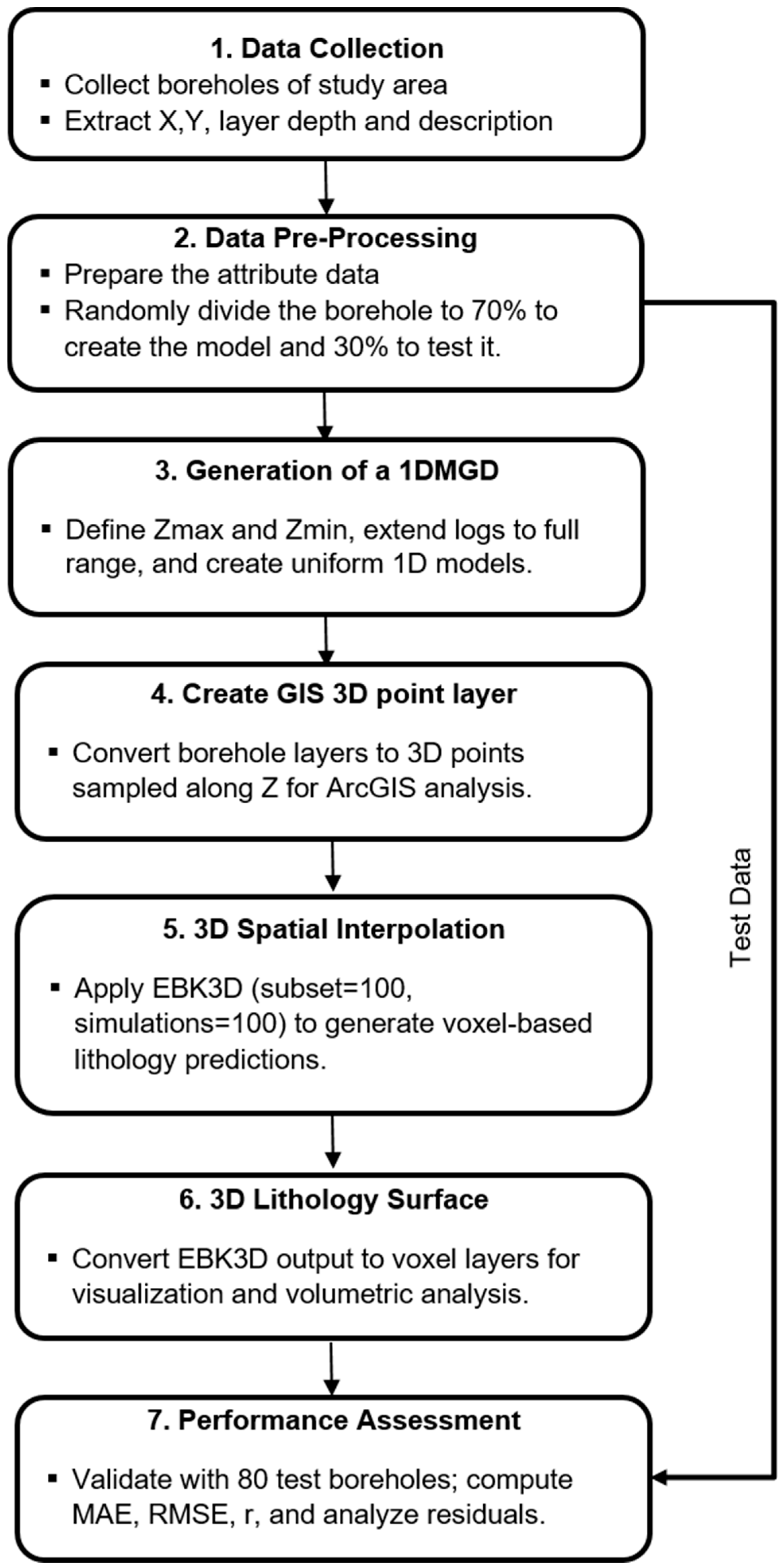
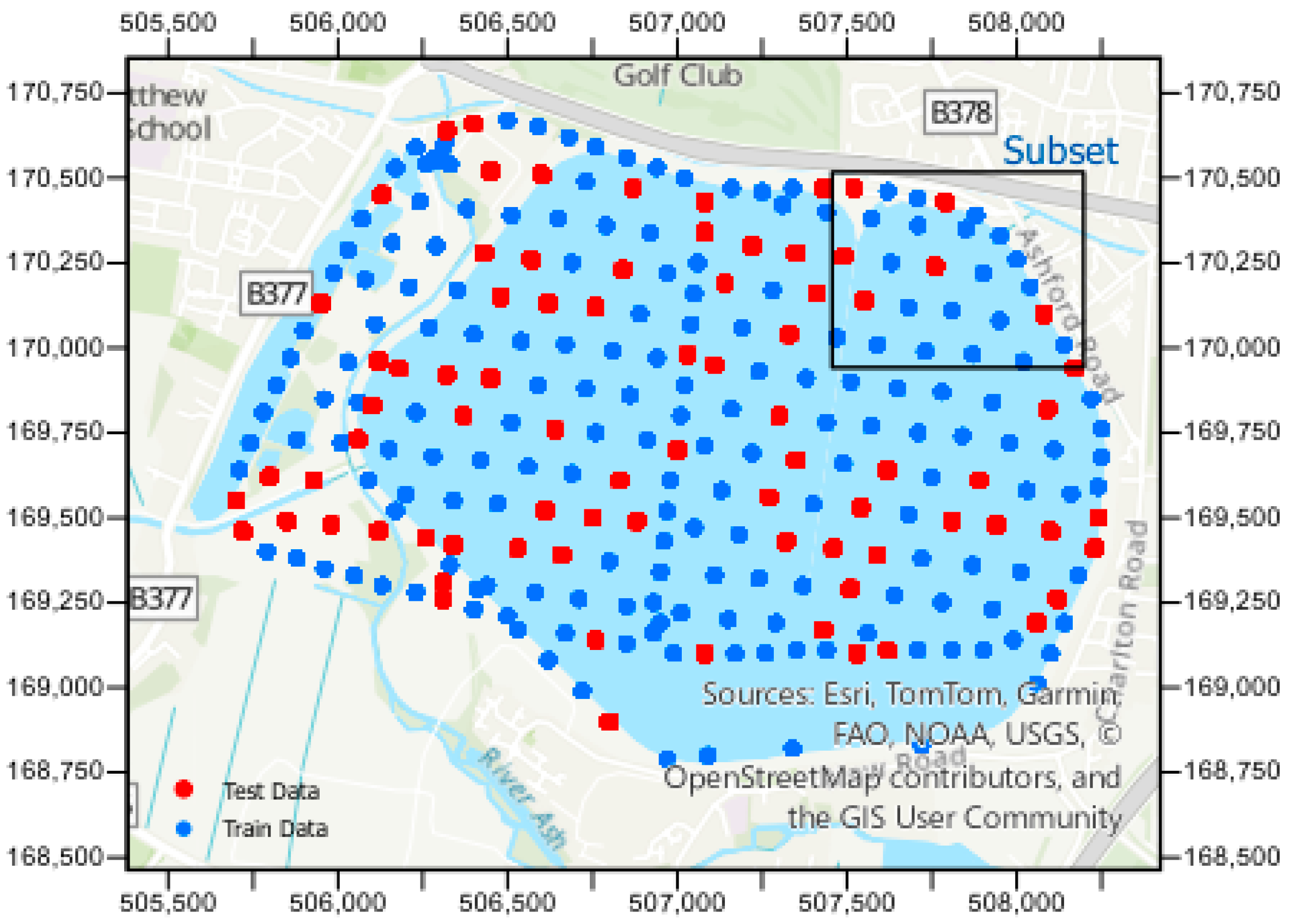
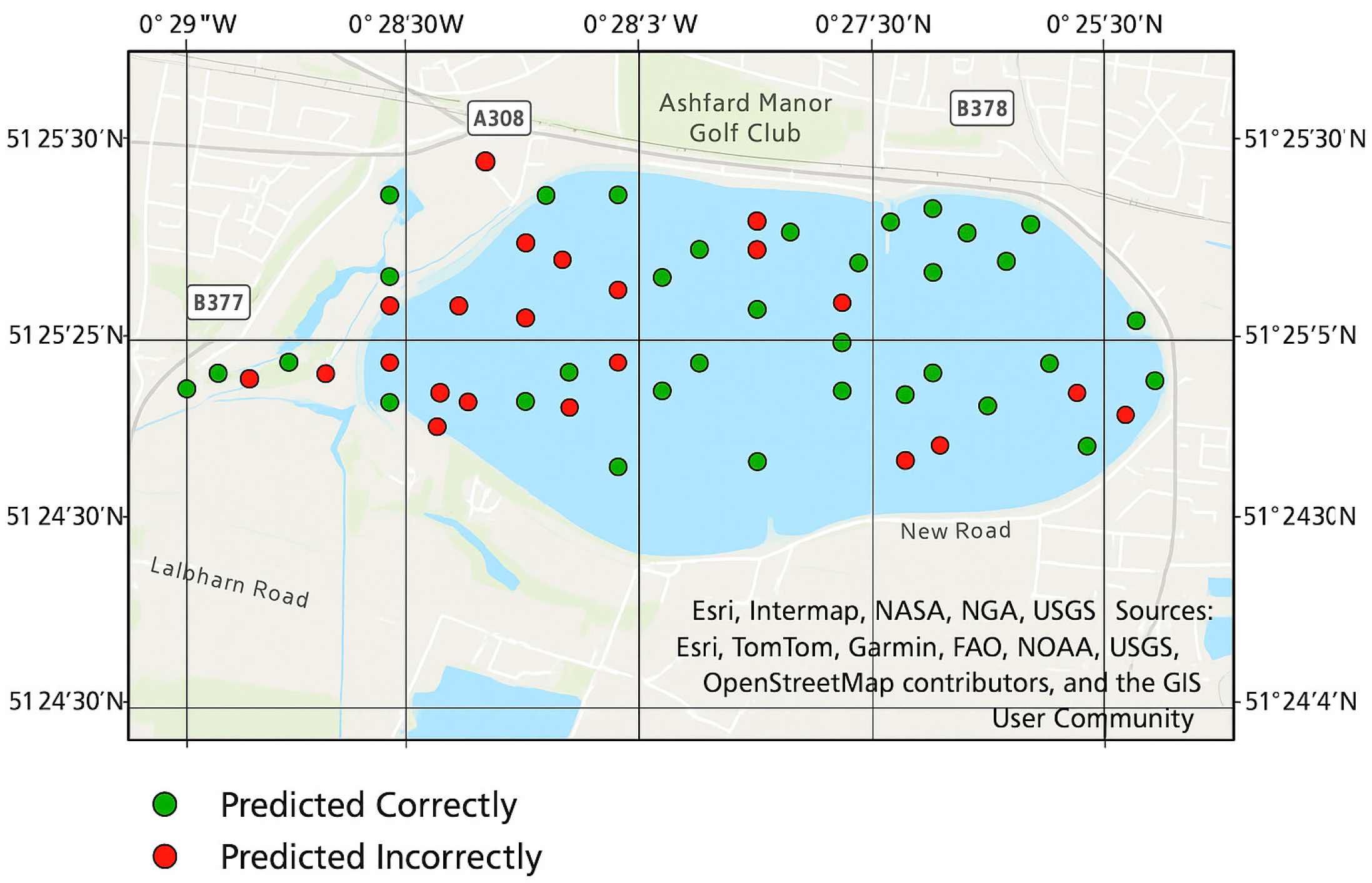
• The 265 boreholes were randomly divided, with 70% (185 boreholes) allocated for interpretation using EBK3D and the remaining 30% (80 boreholes) reserved for validation of interpretation and prediction results on test data, as shown in Figure 3. This random selection ensured proportional representation of spatial and lithological diversity within the study area, thereby minimizing potential spatial bias.

3.3. Generation of a 1DMGD

In this stage, a one-dimensional model of the borehole data (1DMGD) is generated for each borehole in the training dataset, which comprises 185 boreholes and represents 70% of the entire dataset. The procedure for this step is as follows:

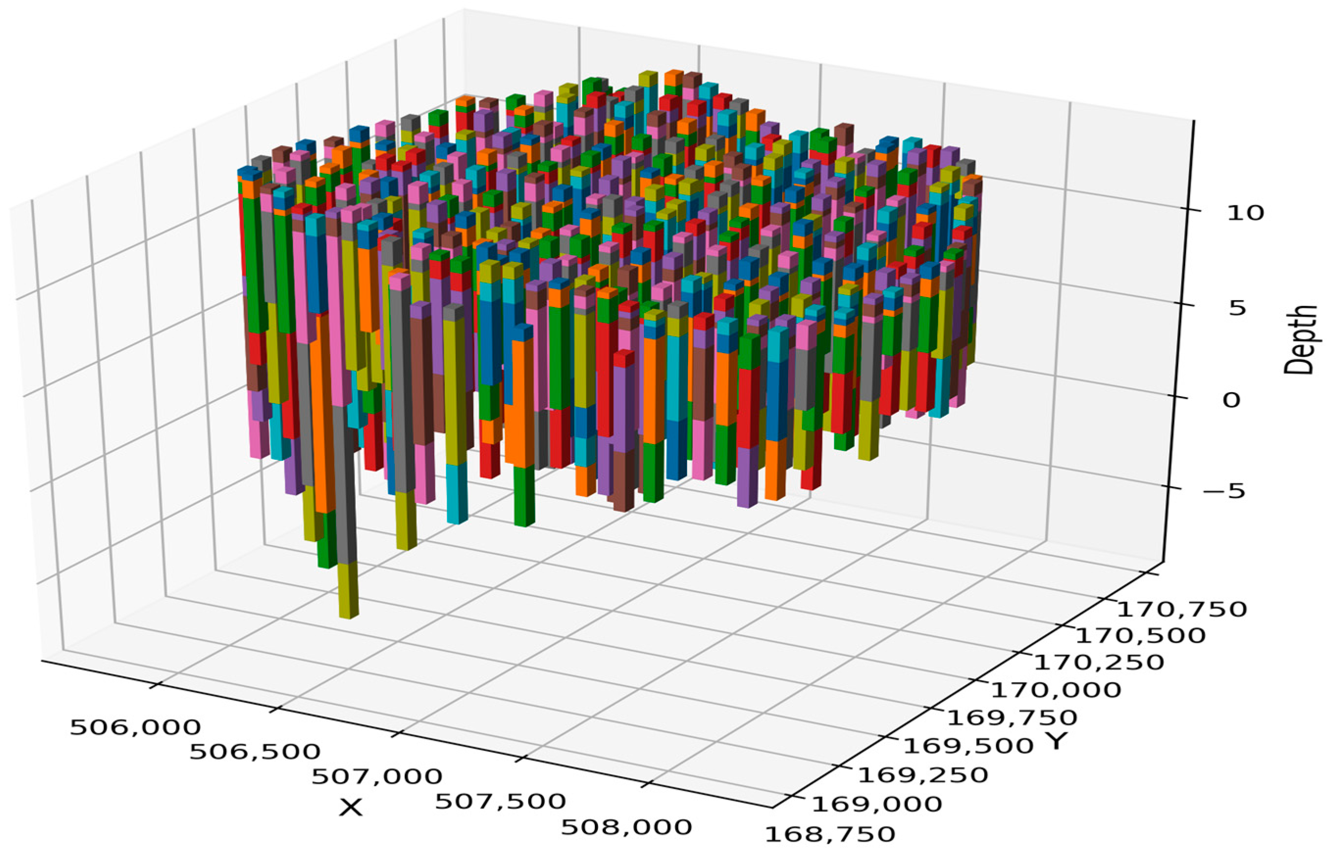
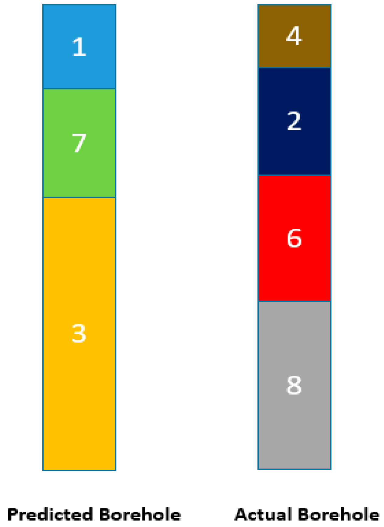
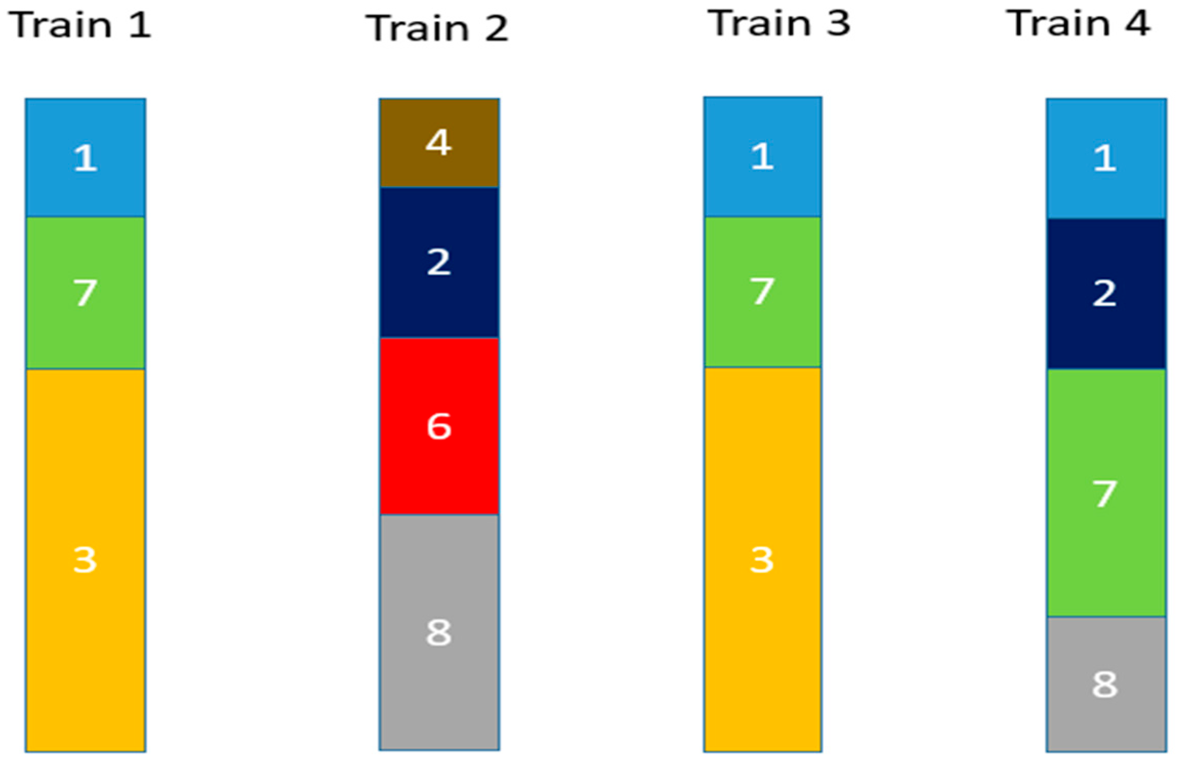
• The boreholes vary in length, top elevation, and bottom elevation, whereas the interpolated voxel layer has a uniform top and bottom as shown in Figure 4. For the training data, Z_min and Z_max are identified, where Z_max is the highest top elevation among the boreholes and Zmin is the lowest bottom elevation. Each 1DMGD is constructed within the range [Z_min, Z_max], which facilitates the generation of a consistent voxel layer of borehole data, as illustrated in Figure 5.
• If the upper end of a borehole log is below Z_max or the lower end is above Z_min, the borehole logs are vertically extended to cover the range [Z_min, Z_max]. In these extended sections, zero is assigned as the integer code to represent NULL, as shown in Figure 5.

3.4. Create GIS 3D Point Layer

The procedure is as follows:

• In GIS, each borehole is represented by multiple points sharing identical X and Y coordinates but differing in Z values. To ensure accurate representation, each lithological layer, including the NULL layer, is depicted by points spaced 10 cm apart.
• For train boreholes, generate a table that includes Borehole-ID, X-coordinate, Y-coordinate, Z-coordinate, and Litho-Code, as illustrated in Figure 5.
• Convert the table to a 3D point layer using ArcGIS Pro 3.2.

3.5. 3D Spatial Interpolation

The literature indicates that 3D spatial interpolation is typically performed by generating a series of horizontal two-dimensional grids at regular intervals of geotechnical data and stacking these grids to construct a three-dimensional spatial model [26,32]. In the present study, a novel approach was implemented by interpolating the 3D point layer using Empirical Bayesian Kriging 3D (EBK3D). EBK3D is a geostatistical interpolation technique that applies the Empirical Bayesian Kriging methodology to three-dimensional point data. The EBK3D model offers a rapid and robust solution for both automatic and interactive data interpolation. Unlike other kriging methods, which require manual parameter adjustment to achieve accurate results, the EBK3D model automatically determines these parameters during the subsetting process and concurrently constructs a robust kriging model [13]. Among the available geostatistical modeling tools, ArcGIS Pro was selected due to its unique implementation of EBK3D, which is not currently available in other commercial or open-source software. This selection facilitated integration with GIS-based workflows and enabled automated parameter estimation, thereby reducing subjectivity in model fitting.

Each input point is required to have X, Y, and Z coordinates, as well as a measured value for interpolation. In this context, the measured value corresponds to the lithology code. The process consists of the following steps:

• A semivariogram model is estimated from the data.
• Using this semivariogram, a new value is simulated at each of the input data locations.
• A new semivariogram model is estimated from the simulated data. A weight for this semivariogram is then calculated using Bayes’ rule, which shows how likely the observed data can be generated from the semivariogram.

Steps 2 and 3 are iteratively repeated during the 3D spatial interpolation process. In each iteration, the semivariogram estimated in step 1 is used to simulate a new set of values at the input locations. The simulated data then inform the estimation of a new semivariogram model and its associated weight [11,13]. The EBK3D parameters listed in

Table 3. Empirical Bayesian Kriging 3D (EBK3D) Parameters.

Parameter	Value
Output type	Prediction
Semivariogram Model Type	Linear
Subset size	100
Overlap Factor	1
Number of Simulations	100
Neighbors to include	1
Include at least	1
Sector type	1 Sector (Sphere)

were selected based on recommendations from the ArcGIS Pro documentation [33], Utepov et al. [34], and iterative testing on the dataset. The parameters for ‘neighbors to include’, ‘include at least’, and ‘sector type’ were each set to 1 to ensure that the interpolation of lithological layers is based on Nearest Neighborhood Interpolation (NNI).

3.6. 3D Lithology Surface

The 3D geostatistical layer generated by EBK3D was transformed into a voxel layer. A voxel layer encodes multidimensional spatial and temporal data within a three-dimensional volumetric visualization. The voxel model partitions three-dimensional space into nonoverlapping, interconnected geometric elements, using voxel data as the fundamental unit to construct the geological model. This data structure also facilitates spatial querying, statistical analysis, and data interpretation [23].

3.7. Performance Assessment

The results of borehole prediction were evaluated by extracting boreholes at the locations of the test data (80 boreholes) from the predicted three-dimensional lithology. The layer type and the elevation of the top of the layers were then compared with the original data. The following methods were used to validate the results [35]:

▪

Percentage of correct boreholes (number of boreholes with the same lithological layers in predicted and actual layers).

Percentage of correct boreholes = (number or correct boreholes/number of total boreholes) × 100.

▪

Percentage of correct lithological layers (number of lithological layers with the same lithology in predicted and actual layers).

Percentage of correct lithological layers = (number or correct layers/number of total layers) × 100.

For the correctly identified lithological layers, the following metrics were calculated [10,12,35]:

• Mean Error (ME)

$$\mathrm{Mean} \mathrm{error}={\displaystyle \frac{{\sum }_{i=1}^n{\widehat{y}}_i-y_i}{n}}$$

(1)

• Mean Absolute Error (MAE)

$$\mathrm{MAE}={\displaystyle \frac{{\sum }_{i=1}^n\left|{\widehat{y}}_i-y_i\right|}{n}}$$

(2)

• Root Means Square Error (RMSE)

$$\mathrm{RMSE}=\sqrt{{\displaystyle \frac{1}{n}}{\sum }_{\ddot{I}=1}^n{\left({\widehat{y}}_i-y_i\right)}^2}$$

(3)

where ${\widehat{y}}_i$ and $y_i$ are the measured and estimated levels.

• Pearson coefficient Correlation (r)
  The Pearson’s correlation coefficient formula is
  $${\displaystyle \frac{\mathrm{n}\Sigma \mathrm{x}\mathrm{y}-(\Sigma \mathrm{x})(\Sigma \mathrm{y})}{\sqrt{(\mathrm{n}\Sigma {\mathrm{x}}^2-{(\Sigma \mathrm{x})}^2)(\mathrm{n}\Sigma {\mathrm{y}}^2-{(\Sigma \mathrm{y})}^2)}}}$$
  In this formula, x is the independent variable, y is the dependent variable and n is the sample size.
• Scatter Plot, Residual Analysis, and Normality Testing

Model validation utilized both graphical and statistical techniques. Scatter plots were generated to compare actual and predicted values, providing a visual assessment of the agreement between observed data and estimates. Points located closer to the 1:1 line indicated higher predictive accuracy. Residual analysis was conducted by calculating the differences between actual and predicted values and plotting them against the predicted values. This facilitated the identification of systematic bias, variance differences, and outliers in model performance. To further evaluate the validity of the predictive model, the distribution of residuals was analyzed. The Shapiro–Wilk normality test was applied to determine whether the residuals followed a Gaussian distribution, a key assumption for geostatistical interpolation and regression-based predictive modeling. Additionally, histograms and Q-Q plots were employed to visually assess the normality assumption.

4. Results

The performance of the proposed EBK3D-GIS framework was assessed in terms of its capability to model three-dimensional lithology and predict borehole stratigraphy. The evaluation includes a presentation of the model’s visual outputs and a quantitative analysis of predictive accuracy under both homogeneous and heterogeneous geological conditions.

4.1. 3D Lithology Model Visualization

A geostatistical layer was generated from borehole data using EBK3D for both the subset area with homogeneous lithological layers and the entire study area with heterogeneous lithological layers. The geostatistical data were converted into a voxel layer to generate a volumetric representation of the subsurface lithology at Queen Mary Reservoir. Figure 6 presents the 3D model, which captures the spatial distribution and interlocking of distinct lithological units. This result demonstrates the framework’s ability to transform point data into a continuous three-dimensional subsurface representation.

4.2. Borehole Prediction

The EBK3D method was applied to generate a geostatistical layer for both the subset and study areas. Predicted borehole data were extracted at the locations of 80 test boreholes in the study area and 6 boreholes in the subset area. In the subset area, which contains homogeneous layers, the extracted boreholes matched the test borehole layers. In contrast, within the study area characterized by heterogeneous layers, only 49% of the test data were accurately interpolated, as illustrated in Figure 7.

Table 4. Classification of test borehole prediction in study area.

Classification	Classes	Number	Percentage
Perfect prediction	All layers are correct	39	48.75%
Minor Errors	Only one layer is incorrect	6	7.5%
	One layer is missing	8	10%
	one layer is extra	6	7.5%
Major Errors	The majority of layers are incorrect (65–80%)	11	13.75%
	Almost half of the layers are incorrect (40–50%)	7	8.75%
	two layers are missing	1	1.25%
Totally Incorrect	All layers are incorrect	2	2.5%
Total		80	100%

and Figure 8 provide an overview of issues encountered with lithological layers in a dataset. It reveals that only 2 boreholes (2.5%) were totally incorrect. 11 boreholes (13.75%) had a majority of incorrect layers (65–80%). Seven boreholes (8.75%) had 40–50% of their layers incorrect. 20 boreholes (25%) had an error in only one layer (extra, missing, or incorrect layer). Table 2 shows that 49% of boreholes were predicted with complete accuracy, while an additional 25% exhibited only minor discrepancies, such as a single missing or extra layer. These results demonstrate that the model accurately represented the overall stratigraphy in 74% of cases.

4.3. Calibration of Incorrect Interpolation

To determine the causes of incorrect predictions within the study area, a single borehole identified as completely mispredicted was selected for further analysis. The test borehole depicted in Figure 9 exhibited incorrect predictions for all stratigraphic layers. Examination of the four nearest boreholes, as illustrated in Figure 10, revealed that the distances from the test borehole to Train Boreholes 1, 2, 3, and 4 were 120, 143, 106, and 136 m, respectively, indicating that Train Borehole 3 is the closest. The profiles of the Train Boreholes, shown in Figure 11, demonstrated substantial differences, highlighting the lithological heterogeneity of the area. The stratigraphic layers of Train Boreholes 1 and 3 are consistent with the model prediction, whereas the actual layers of the test borehole correspond to those of Borehole 2, which is the most distant.

4.4. Lithological Layers Prediction

For homogenous layers, the layers of all test boreholes were predicted correctly. For heterogeneous layers, 269 layers (77%) were predicted correctly, while 79 (23%) layers’ predictions were incorrect. This indicates that the prediction method accurately identified the correct layer in 77% of instances, but there is still a 23% rate of incorrect predictions, suggesting room for improvement in the model.

4.5. Lithological Layers’ Level Prediction

Model performance was assessed for both homogeneous and heterogeneous layers using standard validation metrics. As presented in

Table 5. Results of validation methods.

Validation Method	Homogenous Layers	Heterogeneous Layers
Mean error value	0.04	0.2
Mean absolute error	0.58	0.31
RMSE	0.74	0.41
Pearson Correlation	0.98	0.99

, homogeneous layers exhibited a mean error of 0.04, indicating minimal bias. The root mean square error (RMSE) was 0.74 and the mean absolute error was 0.58, indicating moderate deviations from the predictions. With a Pearson correlation coefficient of 0.98, the anticipated and actual values show a good linear relationship. These measurements are more sensitive to individual prediction mistakes due to the homogenous layer dataset’s relatively short size, which may also increase observed variability. Better prediction accuracy was demonstrated for heterogeneous layers, where the mean absolute error and RMSE were 0.31 and 0.41, respectively, while the mean error was 0.2. A Pearson correlation coefficient of 0.99 means that predictions and observations agree very well. The stability of these measurements is improved and sensitivity to outliers is decreased with a larger sample size for heterogeneous layers. In summary, the model shows strong predictive performance for both kinds of layers, with somewhat better accuracy for heterogeneous layers, which is probably due to the bigger dataset.

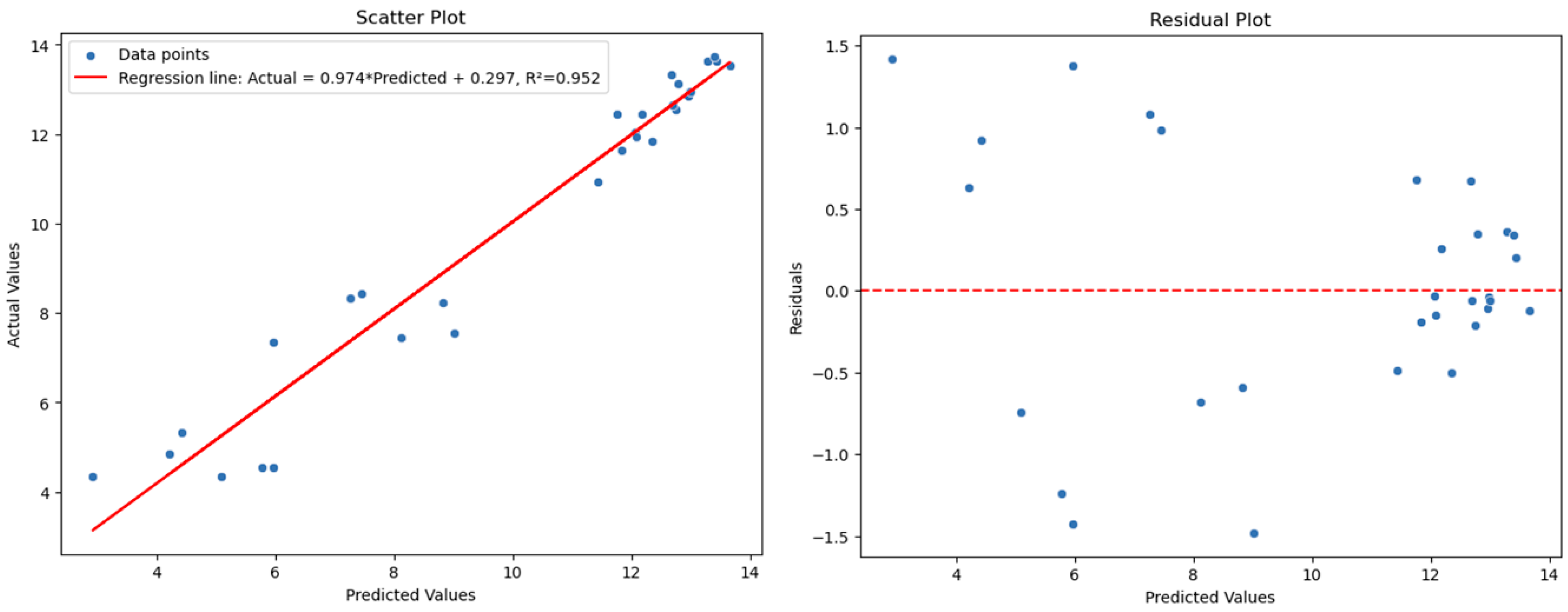
• Scatter plot and residual analysis: The model was evaluated under both heterogeneous and homogeneous lithological conditions. Model performance is compared for homogeneous and heterogeneous lithology in Figure 12 and Figure 13. Although there is a considerable scatter around the regression line in the scatter plot for the heterogeneous scenario (Figure 12), which reflects variability due to the complex nature of heterogeneous subsurface conditions, there is a strong connection between the anticipated and actual values. Localized inaccuracies are indicated by the residual plot, which shows residuals that are unevenly distributed around zero and higher deviations at lower projected values. In contrast, On the other hand, the homogeneous lithology case (Figure 13) shows a closer alignment of points along the regression line, indicating a higher prediction accuracy. The resulting residual map confirms decreased error and improved consistency, with residuals tightly packed around zero with little dispersion. According to this comparison, the model works better under homogeneous settings, whereas predictions are more questionable under heterogeneous lithology.
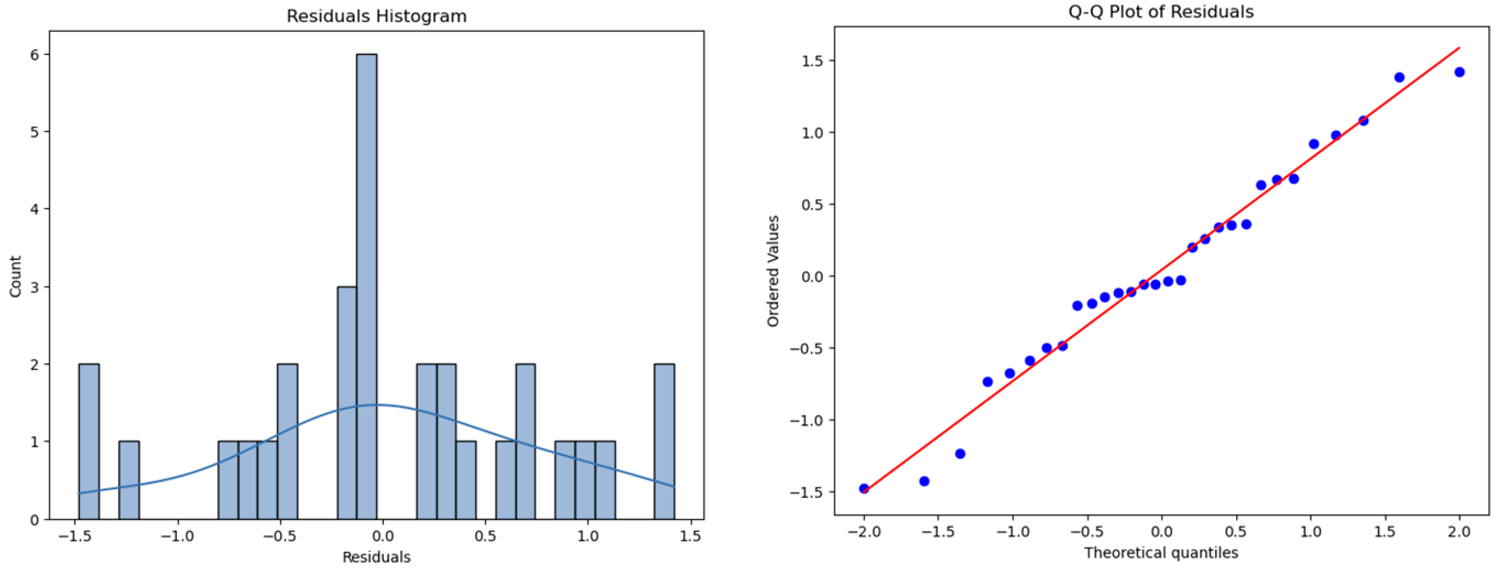
• Shapiro–Wilk test: For homogeneous layers, the Shapiro–Wilk test yielded a p-value of 0.649 and a statistic of W = 0.973. The findings for heterogeneous layers were p-value = 0.0781 and W = 0.9912. These findings imply that the residuals are regularly distributed, indicating that we were unable to rule out the null hypothesis of normality. With data points closely following the 45° reference line, this normal distribution pattern was visually verified using the residual histogram and Q-Q plot in Figure 14 and Figure 15. As a result, the normality assumption of residuals was satisfied, confirming the validity of the model.

5. Discussion

5.1. Advancement in Subsurface Modeling via EBK3D-GIS Integration

The integration of EBK3D and GIS in this study constitutes a substantial advancement in three-dimensional lithological modeling. Traditional interpolation methods, including Inverse Distance Weighting (IDW) and ordinary kriging, are unable to adequately address the complex vertical heterogeneity of subsurface layers and rely primarily on manual parameterization, which introduces subjectivity and limits scalability [13,25]. In contrast, the EBK3D-GIS framework provides robust measures of prediction uncertainty, enables spatial autocorrelation analysis in three dimensions, and automates the variogram fitting process. This automation minimizes expert bias and improves the scalability and reproducibility of subsurface modeling, thereby facilitating broader adoption of advanced geostatistical methods in engineering and environmental applications.

Comparative studies have demonstrated that Empirical Bayesian Kriging (EBK) and EBK3D outperform traditional interpolation methods such as Ordinary Kriging (OK) and Inverse Distance Weighting (IDW). For instance, Al-Mamoori et al. [28] reported that EBK achieved lower root mean square error (RMSE) and higher coefficient of determination (R²) than IDW and OK when estimating soil bearing capacity. Additionally, Li et al. [13] and Zaresefat et al. [12] attributed the improved stability and reliability of predictions for soil contamination and groundwater datasets to EBK3D’s automated variogram fitting and uncertainty quantification. These findings underscore the advantages of EBK3D in modeling complex spatial variability. Future research will extend the current framework to include parallel validation against alternative interpolation techniques for quantitative benchmarking.

5.2. Interpretation of Model Performance and Predictive Capability

The results offer a comprehensive evaluation of the predictive performance of the framework. With a correlation coefficient of 0.99 and low error metrics, such as mean absolute error (MAE) of 0.31 m and root mean square error (RMSE) of 0.41 m in heterogeneous conditions, the model is highly accurate at predicting the elevations of lithological layers. The efficacy of the Empirical Bayesian Kriging 3D (EBK3D) interpolation algorithm in determining likely layer boundaries is validated by this spatial precision.

The model demonstrated a strong ability to represent the spatial distribution of geological materials, achieving 77% accuracy in classifying the types of lithological layers at particular locations. The framework’s robustness was confirmed when it achieved 100% accuracy in predicting entire borehole sequences within homogeneous zones in geologically consistent areas.

5.3. Challenges in Stratigraphic Sequence Prediction

A principal challenge identified in this study is the accurate reconstruction of complete stratigraphic sequences within individual boreholes situated in heterogeneous environments. The 49% overall borehole prediction accuracy draws attention to a basic drawback of all spatial interpolation techniques: stratigraphic similarity is not always guaranteed by spatial proximity.

As illustrated in Figure 9, Figure 10 and Figure 11, a test borehole’s lithology can more closely resemble a more distant training borehole than its immediate neighbor due to abrupt depositional boundaries, channel fills, or other localized variations. This geological context indicates that even highly accurate interpolation algorithms such as EBK3D may generate logically interpolated but stratigraphically incorrect sequences at specific locations when surrounding data points are unrepresentative. The finding that 27% of test boreholes had significant errors is in line with earlier research [26,36] and emphasizes how vulnerable interpolation models are to sudden geological changes and sparse data.

This result accurately reflects the site’s inherent geological complexity rather than pointing to EBK3D’s failure. The output of the model, including its quantification of uncertainty, can be used to pinpoint high-ambiguity areas that most warrant additional site research.

5.4. Novelty and Practical Implications

The useful implementation of the EBK3D algorithm, which is presently exclusive to the ArcGIS Pro platform, for 3D lithological modeling is a significant innovation of this work. Although powerful visualization and interpolation tools are provided by other specialized geological software (such as Leapfrog Geo and RockWorks), these programs usually rely on manual variogram modeling and traditional kriging techniques. An important benefit for reaching efficient and objective modeling results is the automated Bayesian-based uncertainty quantification integrated into EBK3D.

The proposed framework creates a reliable, repeatable, and economical method for converting unprocessed borehole data into a three-dimensional lithological model that takes uncertainty into account. These models are more applicable for cross-disciplinary decision-making in geotechnical design, urban planning, and environmental risk assessment when they are generated in a mainstream geographic information system environment. Infrastructure planning and sustainable development are informed by volumetric calculations and spatial queries made easier by the voxel-based output.

6. Research Limitations

The quality and accessibility of borehole data determine how well the suggested EBK3D–GIS framework predicts subsurface lithology. Prediction reliability is decreased by sparse and unevenly distributed boreholes, particularly in geologically complex areas. Subsurface heterogeneities or subtle lithological transitions may not be sufficiently represented by the framework’s reliance on data from boreholes. The results’ applicability to areas with irregular or sparse sampling is constrained by these data limitations.

A further limitation concerns the methodological scope of the study. EBK3D uses statistical assumptions that might not account for nonlinear geological processes, even though it integrates uncertainty and spatial autocorrelation into interpolation. The framework has not been thoroughly tested using auxiliary datasets that could improve comprehension of subsurface variability, such as geophysical or remote sensing data. As a result, even though the method performs better than traditional interpolation techniques, highly heterogeneous or data-poor environments may cause its predictive accuracy and adaptability to decline.

7. Conclusions and Future Scope

This study presented a GIS-based framework integrating EBK3D to generate volumetric models of subsurface lithology from borehole data. By automatically estimating variogram parameters and integrating spatial autocorrelation and uncertainty into predictions, the framework successfully gets around the drawbacks of traditional interpolation techniques. The model showed excellent accuracy under homogeneous subsurface conditions, predicting lithological layers and boreholes 100% of the time with very little depth error (MAE = 0.58 m, r = 98%). According to these findings, EBK3D works best at locations with stable geology. The model continued to perform well in heterogeneous environments, obtaining high precision in depth prediction (MAE = 0.31 m, r = 0.99) and 77% accuracy in lithological layer identification. 49% of boreholes were correctly identified by the model, with 24% and 27% of them having minor and major errors, respectively. These results highlight the benefits of EBK3D over conventional interpolation methods, especially its ability to measure uncertainty and account for spatial autocorrelation. The sparsity of borehole data and geological heterogeneity, which can affect model precision, are still difficult to handle.

The scope for future research in this area includes the following directions:

▪

Incorporating remote sensing datasets, geophysical survey results, and additional borehole information to reduce data sparsity and enhance spatial resolution.

▪

Combining EBK3D with advanced machine learning and deep learning algorithms to improve predictive accuracy and automate subsurface characterization.

▪

Development of probabilistic uncertainty visualization tools for risk-informed site investigations. These advancements will strengthen the role of geostatistical modeling in sustainable and data-driven subsurface characterization.

References

- Priya, D.B.; Dodagoudar, G.R. An integrated geotechnical database and GIS for 3D subsurface modelling: Application to Chennai City, India. Appl. Geomat. 2018, 10, 47–64. [Google Scholar] [CrossRef]
- Azarafza, M.; Ghazifard, A. Urban geology of Tabriz City: Environmental and geological constraints. Adv. Environ. Res. 2016, 5, 95–108. [Google Scholar] [CrossRef]
- Hademenos, V.; Stafleu, J.; Missiaen, T.; Kint, L.; Van Lancker, V.R. 3D subsurface characterisation of the Belgian Continental Shelf: A new voxel modelling approach. Neth. J. Geosci. 2019, 98, e1. [Google Scholar] [CrossRef]
- Guo, J.; Wang, X.; Wang, J.; Dai, X.; Wu, L.; Li, C.; Li, F.; Liu, S.; Jessell, M.W. Three-dimensional geological modeling and spatial analysis from geotechnical borehole data using an implicit surface and marching tetrahedra algorithm. Eng. Geol. 2021, 284, 106047. [Google Scholar] [CrossRef]
- Nistor, M.M.; Rahardjo, H.; Satyanaga, A.; Hao, K.Z.; Xiaosheng, Q.; Sham, A.W.L. Investigation of groundwater table distribution using borehole piezometer data interpolation: Case study of Singapore. Eng. Geol. 2020, 271, 105590. [Google Scholar] [CrossRef]
- Iwasaki, T.; Arakawa, T.; Tokida, K.I. Simplified procedures for assessing soil liquefaction during earthquakes. Int. J. Soil Dyn. Earthq. Eng. 1984, 3, 49–58. [Google Scholar] [CrossRef]
- Kim, J.; Han, J.; Park, K.; Seok, S. Improved IDW Interpolation Application Using 3D Search Neighborhoods: Borehole Data-Based Seismic Liquefaction Hazard Assessment and Mapping. Appl. Sci. 2022, 12, 11652. [Google Scholar] [CrossRef]
- Wiegel, A.; Peña-Olarte, A.A.; Cudmani, R. Perspectives of 3D Probabilistic Subsoil Modeling for BIM. Geotechnics 2023, 3, 1069–1084. [Google Scholar] [CrossRef]
- Cowan, E.J.; Beatson, R.K.; Fright, W.R.; McLennan, T.J.; Mitchell, T.J. Rapid Geological Modelling; Australian Institute of Geoscientists: Kalgoorlie, Australia, 2002. [Google Scholar]
- Gong, G.; Mattevada, S.; O’Bryant, S.E. Comparison of the accuracy of kriging and IDW interpolations in estimating groundwater arsenic concentrations in Texas. Environ. Res. 2014, 130, 5969. [Google Scholar] [CrossRef]
- Krivoruchko, K. Empirical bayesian kriging. ArcUser Fall 2012, 6, 1145. [Google Scholar]
- Zaresefat, M.; Derakhshani, R.; Griffioen, J. Empirical Bayesian Kriging, a Robust Method for Spatial Data Interpolation of a Large Groundwater Quality Dataset from the Western Netherlands. Water 2024, 16, 2581. [Google Scholar] [CrossRef]
- Li, Z.; Tao, H.; Zhao, D.; Li, H. Three-dimensional empirical Bayesian kriging for soil PAHs interpolation considering the vertical soil lithology. CATENA 2022, 212, 106098. [Google Scholar] [CrossRef]
- Al-Zghoul, S.; Al-Homoud, M. GIS-Driven Spatial Planning for Resilient Communities: Walkability, Social Cohesion, and Green Infrastructure in Peri-Urban Jordan. Sustainability 2025, 17, 6637. [Google Scholar] [CrossRef]
- Al-Homoud, M.; Al-Zghoul, S. Socio-Spatial Bridging Through Walkability: A GIS and Mixed-Methods Analysis in Amman, Jordan. Buildings 2025, 15, 1999. [Google Scholar] [CrossRef]
- Krushnasamy, V.S.; Al-Omari, O.; Sundaram, A.; Varghese, I.K.; Muniyandy, E.; Rao, M.N. LiDAR-Based Climate Change Imaging in Geoscience Using Spatio Extreme Fuzzy Gradient Model. Remote Sens. Earth Syst. Sci. 2025, 8, 465–472. [Google Scholar] [CrossRef]
- Hussain, T.; Abbas, J.; Wei, Z.; Nurunnabi, M. The effect of sustainable urban planning and slum disamenity on the value of neighboring residential property: Application of the hedonic pricing model in rent price appraisal. Sustainability 2019, 11, 1144. [Google Scholar] [CrossRef]
- Azzali, S.; Yew, A.S.Y.; Wong, C.; Chaiechi, T. Silver cities: Planning for an ageing population in Singapore. An urban planning policy case study of Kampung Admiralty. Archnet-IJAR Int. J. Archit. Res. 2022, 16, 281–306. [Google Scholar] [CrossRef]
- Liang, Z.; Qiao, D.; Sung, T. Research on 3D virtual simulation of geology based on GIS. Arab. J. Geosci. 2021, 14, 398. [Google Scholar] [CrossRef]
- Saravanavel, J.; Ramasamy, S.M.; Palanivel, K.; Kumanan, C.J. GIS based 3D visualization of subsurface geology and mapping of probable hydrocarbon locales, part of Cauvery Basin, India. J. Earth Syst. Sci. 2020, 129, 36. [Google Scholar] [CrossRef]
- Pando, L.; Flor-Blanco, G.; Llana-Fúnez, S. Urban geology from a GIS-based geotechnical system: A case study in a medium-sized city (Oviedo, NW Spain). Environ. Earth Sci. 2022, 81, 193. [Google Scholar] [CrossRef]
- Nguyễn, T.-T.; Dong, J.-J.; Tseng, C.-H.; Baroň, I.; Chen, C.-W.; Pai, C.-C. Three-Dimensional Engineering Geological Model and Its Applications for a Landslide Site: Combination of Grid- and Vector-Based Methods. Water 2022, 14, 2941. [Google Scholar] [CrossRef]
- Li, J.; Liu, P.; Wang, X.; Cui, H.; Ma, Y. 3D geological implicit modeling method of regular voxel splitting based on layered interpolation data. Sci. Rep. 2022, 12, 13840. [Google Scholar] [CrossRef]
- Feng, Y.; Wen, G.; Shang, J.; Wen, S.; Wu, B. Research on 3D geological modeling based on boosting integration strategy. Ore Geol. Rev. 2024, 171, 106157. [Google Scholar] [CrossRef]
- Vital, T.R.; Tripathy, G.K.; Mishra, B. A GIS-based borehole data management and 3D visualization system: A case study of Pitisal sand deposit along Puri Coast, Odisha, India. J. Coast. Sci. 2015, 2, 24–28. [Google Scholar]
- Nonogaki, S.; Masumoto, S.; Nemoto, T.; Nakazawa, T. Voxel modeling of geotechnical characteristics in an urban area by natural neighbor interpolation using a large number of borehole logs. Earth Sci. Inform. 2021, 14, 871–882. [Google Scholar] [CrossRef]
- Krivoruchko, K.; Gribov, A. Evaluation of empirical Bayesian kriging. Spat. Stat. 2019, 32, 100368. [Google Scholar] [CrossRef]
- Al-Mamoori, S.K.; Al-Maliki, L.A.; Al-Sulttani, A.H.; El-Tawil, K.; Al-Ansari, N. Statistical Analysis of the Best GIS Interpolation Method for Bearing Capacity Estimation in An-Najaf City, Iraq. Environ. Earth Sci. 2021, 80, 683. [Google Scholar] [CrossRef]
- Volungevicius, J.; Žydelis, R.; Amaleviciute-Volunge, K. Advancements in Soil Organic Carbon Mapping and Interpolation Techniques: A Case Study from Lithuania’s Moraine Plains. Sustainability 2024, 16, 5157. [Google Scholar] [CrossRef]
- Kim, M.; Kim, H.S.; Chung, C.K. A Three-Dimensional Geotechnical Spatial Modeling Method for Borehole Dataset Using Optimization of Geostatistical Approaches. KSCE J. Civ. Eng. 2020, 24, 778–793. [Google Scholar] [CrossRef]
- Available online: https://hatarilabs.com/ih-en/data-extraction-and-spatial-3d-representation-from-bgs-borehole-data-in-ags-format-with-python (accessed on 22 January 2025).
- Khan, M.S.; Kim, I.S.; Seo, J. A boundary and voxel-based 3D geological data management system leveraging BIM and GIS. Int. J. Appl. Earth Obs. Geoinf. 2023, 118, 103277. [Google Scholar] [CrossRef]
- Esri Empirical Bayesian Kriging 3D (Geostatistical Analyst). Available online: https://pro.arcgis.com/en/pro-app/latest/tool-reference/geostatistical-analyst/empirical-bayesian-kriging-3d.htm (accessed on 12 October 2025).
- Utepov, Y.; Aldungarova, A.; Mukhamejanova, A.; Awwad, T.; Karaulov, S.; Makasheva, I. Voxel Interpolation of Geotechnical Properties and Soil Classification Based on Empirical Bayesian Kriging and Best-Fit Convergence Function. Buildings 2025, 15, 2452. [Google Scholar] [CrossRef]
- Adiat, K.A.N.; Nawawi, M.N.M.; Abdullah, K. Assessing the accuracy of GIS-based elementary multi criteria decision analysis as a spatial prediction tool–a case of predicting potential zones of sustainable groundwater resources. J. Hydrol. 2012, 440, 75–89. [Google Scholar] [CrossRef]
- Bamisaiye, O.A. Subsurface mapping: Selection of best interpolation method for borehole data analysis. Spat. Inf. Res. 2018, 26, 261–269. [Google Scholar] [CrossRef]