Abstract
This study evaluates the impact of incorporating lateral mass density variations into geoid models for Java, Indonesia, aiming to enhance the accuracy of regional geoid determinations. Geoid models have traditionally used a constant density assumption; however, Java’s varied topography and geological complexity suggest that density variability may significantly influence geoid accuracy. Employing the Stokes–Helmert method combined with the remove–compute–restore (RCR) technique, we calculated geoid models using both constant density and laterally variable density from the UNB TopoDens model. The models were validated against GNSS/leveling data, showing that while lateral density variations had limited effects along flat topographic profiles, they introduced notable discrepancies in regions with considerable elevation changes. Specifically, variable density models exhibited discrepancies of up to 30 cm in regions with complex terrain, underscoring the importance of selecting appropriate density models for precise geoid computations in heterogeneous landscapes. Nonetheless, a comprehensive validation using geometric geoid models is required to confirm the accuracy improvements across the entire region.
1. Introduction
Geoid modeling is a crucial aspect of geodesy, as it provides a precise representation of the Earth’s gravitational field. A regional geoid model is typically determined by combining gravity anomalies and a global geopotential model, following Stokes’ approach. In the case of Stokes’ approach, the observed gravity data on the Earth’s surface must be reduced to the geoid. This procedure requires mass density information between the geoid and topographic surface [1]. The approximation of the worldwide mean crustal density value has nearly entirely been a constant value of 2670 kg m−3 [2]. However, recent studies highlight the importance of accounting for actual density variations, which can differ by as much as ±20% from the assumed constant value [3].
The application of laterally variable topographic density models in gravimetric geoid computations has been the subject of several studies in the past [4,5]. Theoretically, it has been assessed that small density variations in mountainous regions can cause geoid undulations and gravity reductions exceeding one decimeter, as calculated using the rectangular prism method [6]. The analysis focused on the effects of lateral density anomalies and approximated the topography using this approach. In central Australia, the impact of surface density variations on modeling terrain effects was investigated by Tziavos and Featherstone [4]. They concluded that even small changes in density can alter the gravimetric geoid by more than 10 cm. In the Canadian Rocky Mountains, the effect of density fluctuation on geoid heights can introduce errors ranging from several centimeters to a decimeter, according to Huang et al. [7]. Similarly, Sjoberg [8] discovered that such errors can range from 2 cm at Lake Baikal to 178 cm at Mt. Everest. Additional research conducted in Iran by Kiamehr [9] shows that variances in crustal density from geological maps can result in differences between real and homogeneous densities in mountainous areas of up to 10–20%. In the Taurus Mountains of Turkey, recent research by Abbak [10] revealed that density variations derived from the crustal model can result in errors of up to three decimeters in geoid calculations. He highlighted the necessity of accurately accounting for density values in geoid modeling.
Following prior investigations into lateral density variations, recent advances have concentrated on more rigorous topographic gravity modeling approaches and the inclusion of vertical density variations to improve geoid accuracy. More recently, Lin and Li [11] applied a rigorous tesseroidal topographic gravity modeling method together with the global lateral topographic density variation model (UNB_TopoDens) in a rugged region of Colorado, USA. Their results showed that considering lateral density variations could change geoid heights at the centimeter level, emphasizing the significant impact of density heterogeneity on precise geoid modeling. In another related study, Lin, Denker, and Müller [12] developed a tesseroid-based method incorporating vertical density variations modeled up to cubic order, enabling the accurate computation of gravitational potential, gravity vector, and gravity gradient tensor values. Validated in the Himalaya region, this approach demonstrated the importance of representing both horizontal and vertical density heterogeneities for precise geoid and gravity field modeling.
The insights from those studies highlight the necessity of integrating detailed lateral and vertical density information into geoid modeling, naturally leading to the challenge of determining accurate crustal density values in practice. Determining the actual crustal density value in a project area presents a significant challenge for researchers due to the need for meticulous care and specialized experiments when computing the density effect on the geoid. Recently, the development of Global Crustal Models (GCMs) has advanced significantly. After overcoming initial challenges, the University of California, San Diego team produced Crust 1.0 at a 1 × 1° resolution [13]. Subsequently, the University of New Brunswick team developed the UNB_TopoDens model, a higher-resolution GCM at 30"× 30", using the Global Lithology Model (GLiM) [14].
As an archipelagic nation, Indonesia features a wide variety of topographical landscapes, including mountains, valleys, and plains. In mountainous areas, these diverse features lead to considerable variations in subsurface mass density. Therefore, accurately determining the range of density values is essential for effective geoid modeling in the region [15]. Presently, geoid modeling in Indonesia is primarily based on the assumption of a uniform topographic mass with a constant density of 2670 kg m−3 extending from the topographic surface to the geoid. However, Indonesia’s intricate topographical and geological characteristics present a valuable opportunity to improve geoid precision by integrating more accurate density estimations. This study investigates the impact of laterally varying average densities on geoid modeling, focusing specifically on Java Island, which is a region characterized by highly variable topography. The approach separates lateral density variations into two components: a constant reference density ( kg m−3) and the UNB TopoDens density model (), which accounts for lateral variability. By systematically evaluating the influence of these density variations, this study aims to enhance the precision and reliability of the geoid model, addressing the critical need for improved geoid performance in Indonesia’s complex topographic landscape.
Although several studies worldwide have addressed the effect of lateral density variations on geoid models, this topic remains underexplored in Indonesia. Given Java’s complex tectonic and topographic conditions, this study fills a critical gap by applying a high-resolution density model to geoid computation and assessing its implications for vertical reference systems in the region.
2. Study Area and Data Description
2.1. Study Area
The study area was Java Island, Indonesia, which is bounded by southern latitudes 6° to 10° and eastern longitudes 104° to 116°. This region includes numerous volcanic peaks and lowland areas with significant elevation differences ranging from sea level to approximately 3676 m above sea level (masl) at the summit of Mt. Semeru (represented by a triangle gradient in Figure 1). The average elevation of the study area is about 500 m. Java is also characterized by active tectonic features and fault systems, contributing to its complex geological structure [16]. These characteristics make Java a relevant and challenging test region for evaluating the effect of lateral mass density variations on gravity reduction and geoid modeling.
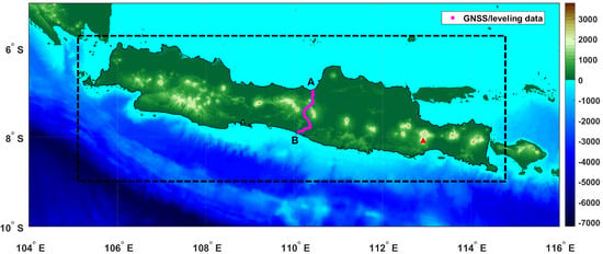
Figure 1.
Topography of the study area with the dashed line indicating the border of the target area. The red triangle represents the location of Mt. Semeru. The GNSS/leveling measurement route is shown, crossing from Semarang (A) to Yogyakarta (B).
Java was selected as a preliminary study area due to its comprehensive and high-quality geospatial data coverage, even though its geographical extent and lateral density contrast are moderate compared to larger tectonically active regions.
2.2. Gravity Data
This study utilizes terrestrial gravity data provided by the Geospatial Information Agency of Indonesia (BIG). The dataset was primarily collected in 2019, supplemented by additional measurements from 2017 at key locations, including Majalengka and Surabaya, using CG-5 and CG-6 Scintrex gravimeters at 2.5–3 km intervals. Data collection focused on major urban centers throughout Indonesia, specifically in Banten, Jakarta, Bandung, Purwokerto, Semarang, Yogyakarta, and Surabaya. Multiple measurement locations within these urban areas were established to facilitate a comprehensive regional assessment. The position of the terrestrial gravity points was determined using GNSS observations defined in the Indonesian Geospatial Reference System 2013 (SRGI2013; [17]). The dataset consists of a total of 1885 data points (see Figure 2).
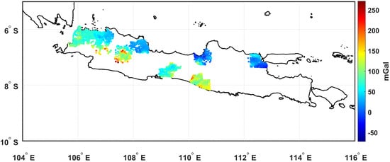
Figure 2.
Distribution of terrestrial free-air gravity data.
Airborne gravity data were used to fill gaps in the terrestrial gravity dataset and were obtained from Bramanto et al. [18]. The survey was conducted using a LaCoste and Romberg Air/Sea Gravity Meter Type S-130, which was mounted on a Cessna Grand Caravan 208b aircraft. Primary flight lines were oriented north–south with a spacing of 15 km and complemented by east–west cross lines to ensure data coverage and quality. Data acquisition took place at an average flight altitude of approximately 4200 m [18]. In principle, the nominal accuracy of an airborne gravity survey can reach up to 1 or 2 mGal. However, factors such as atmospheric turbulence, wind variations, and aircraft motion dynamics impacted measurement stability and ultimately reduced accuracy. The accuracy of airborne gravity data used in this study was estimated to be 3.37 mGal based on the standard deviation of the crossover difference. Further details regarding the setup of airborne gravity survey can be seen in the study of Bramanto et al. [18].
The original dataset consisted of 196,601 data points with an interval of approximately 70–80 m along the track (see Figure 3). However, due to the computational burden, we resampled the data with an interval of about 350–400 m along the trajectory line. This process reduced the data to 9831 points. Note that this process could attenuate the high-frequency components of the gravity signal. Nevertheless, the reduction in data density is not expected to impact the accuracy significantly given that the spatial resolution target of the calculated model is one arcminute or about 2 km.
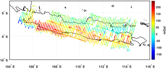
Figure 3.
Distribution of airborne free-air gravity data.
Finally, marine gravity data obtained from the Technical University of Denmark’s DTU17 model, with a resolution of 1 arcminute, are utilized to analyze the coastal regions around the study area. The DTU17 marine gravity model integrates data from the SARAL/AltiKa geodetic mission, which commenced in 2016, along with enhanced Arctic processing from the Cryosat-2 mission, providing global geodetic data every 369 days with an 8 km resolution since its launch in 2010 [19]. Additionally, DTU17 incorporates geodetic data from the Jason-1 mission conducted in 2012 and 2013. Globally, the DTU17 marine gravity model exhibits a standard deviation of 2.51 mGal compared to marine gravity control points in the North Atlantic Ocean and 3.78 mGal compared to airborne gravity observations in the Arctic Ocean [20].
2.3. Digital Terrain Model
Topography data from the Digital Terrain Model (DTM) serves as the short-wavelength component of terrain data, which is essential for assessing terrain gravity effects. High-resolution DTM data are sourced from the Shuttle Radar Topographic Mission (SRTM) [21]. The SRTM 3 arcsecond model provided high-resolution data for land areas [22]. The second dataset used in this study is the SRTM15+ global bathymetry model, which is an advanced version of the SRTM+ series [23,24]. The SRTM15+ model [25] offers comprehensive global coverage with a spatial resolution of 15 arcseconds. This study utilized a combination of the SRTM 3 arcsecond and SRTM15+ models to cover both land and ocean regions.
We further assessed the performance of the SRTM 3 arcsecond elevation data by comparing it to orthometric heights derived from GNSS/leveling observations, as shown in Figure 4. The correlation coefficient (r) of 0.9996 indicates a strong positive linear relationship between the topographic profile and the GNSS/leveling data, suggesting a high degree of consistency. The differences between the orthometric heights of the SRTM 3 arcsecond data and the GNSS/leveling validation points ranged from −33.819 to 32.728 m with an average difference of 4.119 m. The standard deviation of these height differences was estimated to be 4.980 m. It is important to note that this evaluation was limited to land areas.
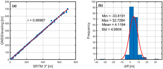
Figure 4.
Correlation of the topographic profile along the validation line with GNSS/leveling data (a), frequency distribution of differences between GNSS/leveling and SRTM 3 (b).
2.4. Topographic Mass Density Model
The primary aim of the study was achieved using the UNB_TopoDens model, which is the first global topographical density model incorporating lateral variation. This model was derived using the Global Lithology Model (GLiM), which applies a high-resolution lithological map [14]. By assigning probable surface density values and error estimates to lithologies based on geological data, GLiM was transformed into UNB_TopoDens. This model is available at three different grid spacings and can be accessed at https://gge.ext.unb.ca/Resources/TopographicalDensity/ (accessed on 15 August 2025).
Figure 5a displays the global UNB_TopoDens model (), where land density values range from 2074 kg m−3 to 2791 kg m−3, with a mean of 2391 kg m−3. This variation reflects the lateral changes in surface density across different geological formations based on the Global Lithology Model (GLiM). The wide range of density values highlights the Earth’s heterogeneous surface composition, which is crucial for accurately modeling topographic effects on gravity. The mean value of 2391 kg m−3 aligns with typical densities for mixed sedimentary lithologies, as reported by [26], confirming that the model effectively represents average global surface densities while accounting for regional anomalies, particularly in the land area of Java Island. Differences in densities () and () range between kg m−3 and kg m−3 with a mean difference of kg m−3. The standard deviation of the difference is kg m−3, indicating moderate variability, which reflects the heterogeneous geological materials of the region.
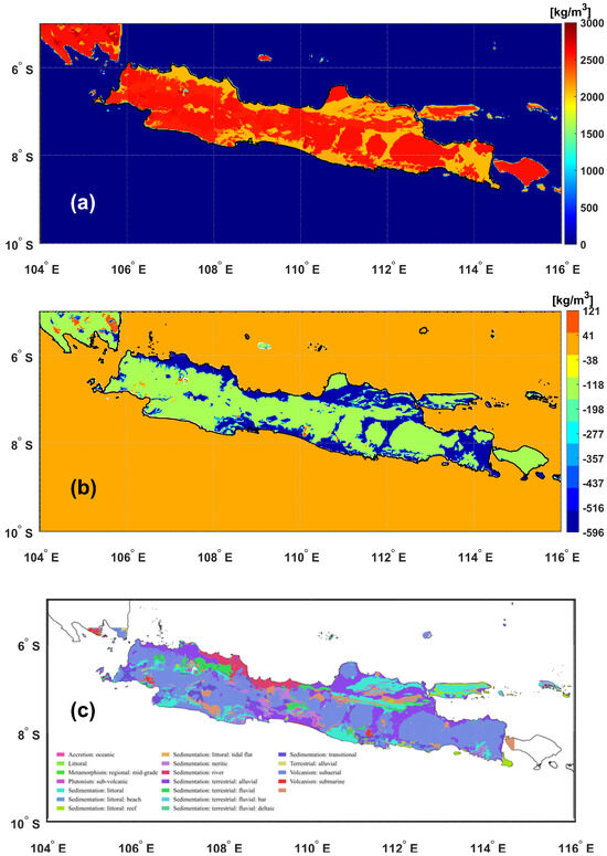
Figure 5.
UNB_TopoDens_2v01 laterally varying topographical density model (a), the difference between and (b), and the geological map of the study area (c).
3. Method
3.1. Data Preparation
The calculation process starts by reducing the observed gravity from terrestrial measurements, taken from the Earth’s surface to the geoid, to derive the free-air gravity anomaly. This process involves compressing all topographical mass above the geoid into a geoid based on Helmert’s 2nd condensation method. The observed gravity is adjusted to the geoid surface using a free-air gravity gradient, resulting in the free-air gravity anomaly (). Mathematically, the free-air gravity anomaly is expressed as [18,27]:
In this context, represents the free-air gravity anomaly derived from terrestrial and airborne gravity observation data, denotes the observed gravity from terrestrial and airborne gravity measurements, is the normal gravity on the reference ellipsoid, is the free-air gravity correction, and is the atmospheric correction.
We need to establish the expected accuracy of the dataset by understanding how the gravity data observations were collected. This helps us determine the limitations of the equipment and methodologies used. An outlier might suggest a unique characteristic of the sample or a mistake. Such outliers should be resolved or removed as they can disproportionately affect surrounding data points [28]. Outlier detection and removal are performed only on terrestrial and airborne gravity data observations () because altimetric gravity data are derived from the global ocean gravity model DTU17. This process aims to eliminate all known contributions to the gravity field to produce a residual gravity field that is statistically more consistent and smoother [29].
In their research, [29] present a comprehensive approach for detecting and removing outliers from gravity data collected through terrestrial and airborne measurements. This method includes computing the median (MED) and median absolute deviation (MAD) of the residual gravity anomaly . The MAD is adjusted by multiplying it by a factor of 1.4826, based on the assumption of normal distribution, to produce the normalized MAD (NMAD). Outliers are determined based on the condition that data values should lie within the interval . After removing these outliers, the missing data are interpolated and compared to the original values. Then, the threshold is determined using the cumulative distribution function and selected based on the 95% percentile.
3.2. Topography Effect on Geoid Computation
Free-air gravity anomalies are obtained by reducing gravity measurements from the Earth’s surface to the geoid without accounting for surface topography effects, such as mass density (), and only considering height (H). Bouguer gravity anomalies are determined to smooth the free-air gravity anomalies in the study area by converting them into Bouguer anomalies. This process aims to remove effects on gravity caused by factors such as surface topography or variations in the Earth’s mass density [30]. In this approach, Bouguer gravity anomalies are approximated using planar Bouguer anomalies with the assumption that density variations can be approximated by flat layers parallel to the Earth’s surface. To determine free-air gravity anomalies from Bouguer anomalies, the following equation is used [31]:
where represents the free-air gravity anomaly in the study area, represents the Bouguer gravity anomaly, and represents the planar Bouguer gravity effect. G is the gravitational constant, is the orthometric height at the observation point p, and is the density value. In this study, a constant topographic mass density value of and the UNB_TopoDens model are used for land areas, and (calculated as the topographic mass density minus the mass of seawater) is applied for marine areas.
Terrain effects are most significant near the computation point and diminish with increasing distance. Therefore, terrain effects are integrated only within a specified radius, which is typically up to 200 km. Terrain correction uses height information from digital elevation models SRTM 3" (z). Consequently, calculating terrain effects demands substantial computational resources. The purpose of this process is to account for the gravitational influence of topography (terrain correction) while simultaneously removing the simplified planar Bouguer slab effect B. The analytical formula for terrain correction (), which is added to Equation (2), is given by the following [32]:
where , , and represent the infinitesimal volume element over which the integration is performed.
The calculation of the indirect topography effect involves removing the Helmert topographic mass, which refers to the phenomenon where there is a reduction of mass in areas with higher elevations (mountains) and an addition of mass in areas with lower elevations (valleys) [33]. The value of the indirect topography effect () is formulated with the following equation:
where R is the Earth’s average radius, and h is the computation height.
The calculation of the indirect effect on the geoid involves restoring the condensed Helmert mass. The value of the first-order indirect effect, , is formulated as follows [34,35]:
The second-order indirect effect, , is given by [34]:
where h is the height of the data point, is the height of the computation point, and indicates the surface element.
3.3. Geoid Computation Using Stokes–Helmert’s Method
In geoid modeling, Stokes’ formula is a well-known method for calculating geoid undulations by performing numerical integration over the entire spherical surface. However, this process is challenging when gravity measurements are restricted to the study area, as is often the case with terrestrial and airborne gravimeters. To address this limitation, the remove–compute–restore (RCR) technique is commonly used in local or regional geoid modeling with a modification for Stokes’s kernel. The RCR method initially removes both long-wavelength components, as predicted by global geopotential models (GGMs), and short-wavelength components, as derived from topographic models, from the observed gravity data. The process of removing long-wavelength components involves eliminating these components, which are represented by global geopotential model gravity anomalies . Residual gravity anomalies are computed by combining Bouguer anomalies, terrain corrections, indirect topography effects, and removing long-wavelength components from EGM2008:
To prepare residual gravity anomalies for geoid calculations, data are gridded using the Least-Squares Collocation (LSC) method [36,37]. The LSC approach is presented in two forms: one that characterizes the relationship between observed data and estimated parameters using a cross-covariance matrix and another that describes this relationship through linear matrix equations.
The first step is to determine the cross-covariance matrix of the observation points and the computation points. To establish the cross-covariance matrix, the empirical model from the observation data will be approximated using an analytical model. This approximation is performed using Hirvonen’s equation. The analytical and empirical models are shown in Figure 6. The equation of the analytical model that fits the obtained empirical model is as follows [38]:
where d is the three-dimensional distance between two data points, between the observation and the computation point, is the covariance value when or the mean of the variance, and and p are the correlation length and cofactor, respectively, determined by trial and error until an analytical model that fits the empirical model is obtained.
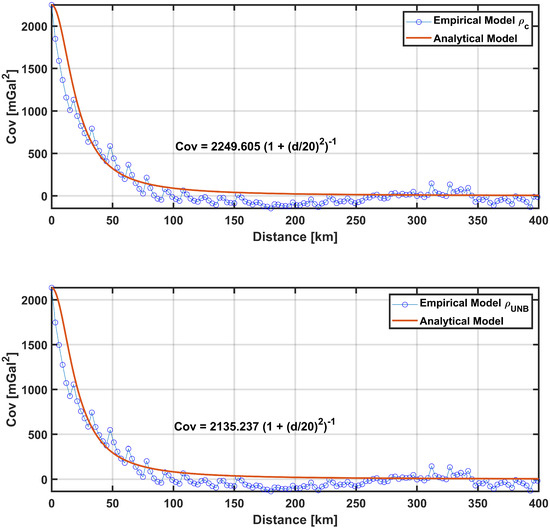
Figure 6.
The empirical model approach using the Hirvonen equation for the constant density model (top) and for the variable density model (bottom).
After isolating the residual gravity field, Stokes’ integration is applied to compute the residual geoid undulations. Once this is complete, the removed long and short-wavelength components are restored to obtain the full geoid model, representing all wavelength contributions [39,40].
The residual Faye gravity anomaly is obtained by restoring Bouguer anomalies that were removed during the smoothing of free-air gravity anomalies in the study area, , in a uniform grid format, . In this step, the Bouguer gravity anomalies previously computed are restored using the following equation:
The calculation of geoid residual values aims to predict the geoid from gravity data. The computations for geoid undulation were performed using GRAVSOFT software, which employs the 1D FFT (Fast Fourier Transform) method to apply the Stokes function with Wong–Gore modifications, adjusting it within a specified range [41]. This method involves modifying the original Stokes function by removing the lowest harmonics, thereby minimizing the influence of local data on longer wavelengths [42,43]. The Wong–Gore modification was selected in this study due to its well-established theoretical basis, widespread application, and proven numerical stability in geoid modeling [44,45].
The modified Stokes function, , is calculated as follows:
In this equation, is Stokes’s kernel, is the radius of the spherical cap at each computation point, M is the degree of the spheroidal adjustment for kernel integration, and denotes the Legendre polynomial. The data used for the geoid residual calculation are the residual Faye gravity anomaly, :
In this context, represents the residual geoid height, R denotes the average Earth radius, refers to the normal gravity, and is an element of the surface. The reference geoid undulation is obtained from EGM2008 and restored to add back the long-wavelength component as follows [46]:
while the long-wavelength component of the gravity anomaly can also be computed as
where is the reference geoid undulation, while is the GGM gravity anomaly at the corresponding geocentric distance, latitude, and longitude, respectively . n and m are the degree and order of GGM spherical harmonics. a is the semi-major axis of reference ellipsoid, M is the mass of the Earth, and are the fully normalized spherical harmonics of the anomaly potential, is the fully normalized Legendre function, and is the maximum degree of the GGM.
Finally, the Stokes–Helmert RCR geoid model is created by combining all the geoid components gathered from the previous steps, as follows:
4. Results and Discussion
4.1. Outliers Detections
The preliminary step in processing the gravity data involved detecting and eliminating biases and outliers. Specifically, 1905 terrestrial and 9831 airborne gravity data points were subjected to the outlier detection process. Outlier detection in terrestrial gravity data identified 70 candidate outliers based on a 95% confidence interval. For the residual gravity anomaly data from terrestrial measurements, a threshold of mGal was determined, leading to the identification of 19 outliers, as shown in Figure 7. These outliers were subsequently removed from the data. Outliers in terrestrial gravity data are primarily observed in the western part of Java, specifically in densely populated cities. These outliers can arise from various factors, including measurement errors such as data recording mistakes, environmental factors like extreme weather or magnetic disturbances, local geological conditions including unusual rock formations and fault zones, and nearby large objects or heavy sources that might interfere with measurements [47]. Identifying and addressing these issues is crucial for ensuring the accuracy of gravity data. Nevertheless, noticeable data gaps remain over certain land areas, which pose challenges in geoid computation. We acknowledge that more advanced treatments are needed to better handle these gaps, and as part of the future outlook, we plan to implement improved gap-filling techniques and adaptive gridding methods to reduce the impact of incomplete data coverage on geoid modeling.
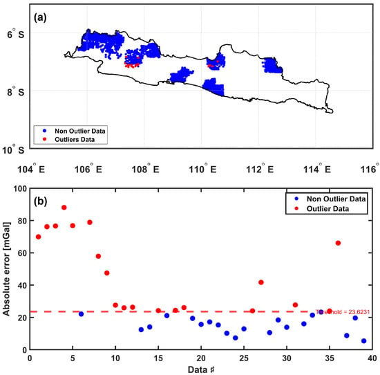
Figure 7.
Spatial distribution of outliers in terrestrial gravity data (a), and outliers detection in terrestrial gravity data (b).
In the airborne gravity data, 413 candidate outliers were detected. A threshold of mGal was established for the residual gravity anomaly from airborne observations, resulting in the detection of 42 outliers, as illustrated in Figure 8. These outliers were also removed from the dataset.
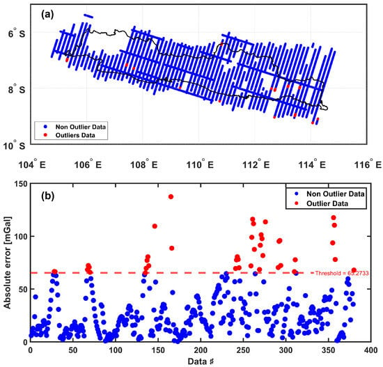
Figure 8.
Spatial distribution of outliers in airborne gravity data (a), and outliers detection in airborne gravity data (b).
Outliers in airborne gravity data can occur due to several factors. Instrument errors, such as calibration issues or equipment malfunctions, can cause unusual readings. Atmospheric changes, like extreme pressure or temperature shifts, may also affect measurements. Movement and vibrations of the aircraft, as well as air turbulence, can lead to inconsistent data. Errors in positioning and interference from large objects below the aircraft can further contribute to anomalies. Ensuring accurate airborne gravity measurements requires addressing these potential issues [48].
This visual representation highlights the range and distribution of the cleaned dataset, providing insights into its characteristics. In the geoid computation process, the data used are merged gravity data, which are subsequently written as , as shown in Figure 9. Additionally, Table 1 summarizes the statistical results of the free-air gravity anomaly values derived from these observations.
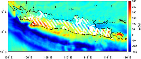
Figure 9.
Distribution of gravity data and free-air gravity anomaly values from terrestrial, airborne, and altimetric gravity observations.

Table 1.
Statistics of different types of gravity anomalies after outlier removing of the database (mGal).
4.2. Downward Continuation and Gridding of Residual Gravity
Downward continuation and gridding were carried out using gravity data that had been cleaned of outliers. This process involved 264 terrestrial gravity measurement points, 9,658 airborne gravity measurement points, and altimetric gravity data with a one-arcminute resolution in marine areas. The computations were based on the residual gravity anomaly values from all the gravity measurements. The first step is to determine the cross-covariance matrix between the observation points and the computation points. To compute the cross-covariance matrix, the empirical model of the observation data is approximated using an analytical model. This approach employs the Hirvonen equation, as referred to in Equation (8). The analytical and empirical models are illustrated in Figure 8, showing both constant density and variable density models with and . The covariance values for the constant density model () are , and for the variable density model (), .
The residual gravity anomalies vary across topographic features, as shown by the blue regions in Figure 10, which denote the high plateaus and mountain peaks. The statistical analysis of residual gravity anomalies shows noticeable differences between the constant density model and the variable density model. For the constant density model (), anomalies range from mGal to mGal, with an average of about mGal, and a standard deviation of mGal. The variable density model (), on the other hand, has a smaller range from mGal to mGal, with an average of mGal, and a standard deviation of mGal.
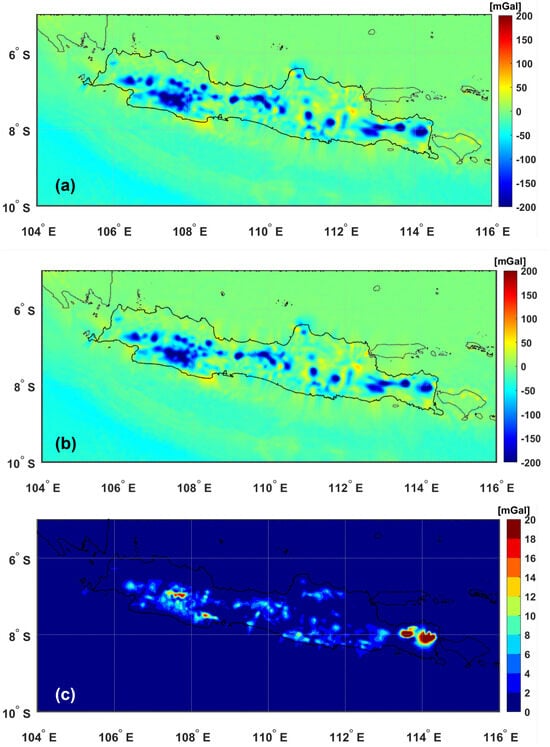
Figure 10.
Spatial distribution of the residual gravity anomalies: with density (a), with density (b), and the difference between the residual gravity anomalies with densities and (c).
The differences between the two models range from mGal to mGal, with a mean difference of mGal. The small standard deviation indicates that the models are quite similar, though some differences persist, particularly in areas with significant topography, as observed in Figure 10c.
4.3. Geoid Computation
The gravimetric geoid model is produced by adding the residual geoid undulation, the indirect impacts of both first- and second-order effects, the short-wavelength components, and the reference geoid undulation values derived from EGM2008. The geoid model created for this investigation has a resolution of 1’. The resolution of the terrestrial gravity data, which has a data interval of 5 km (1’), is considered when using a 1’ resolution. In the geoid computation using the Stokes method with a 1D FFT approach, an evaluation was performed to determine the optimal spherical cap radius and degree M. As shown in Figure 11, the evaluation led to the selection of a spherical cap radius and Wong–Gore degree . This choice produced various geoid models, resulting in a geoid model with a standard deviation of 10.74 cm for and 10.67 cm for .
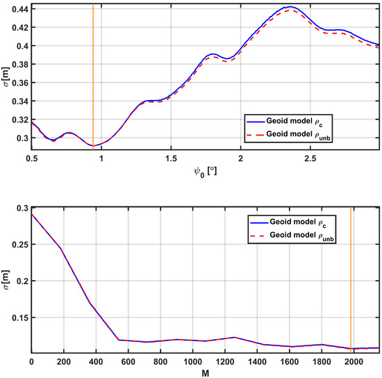
Figure 11.
Evaluation of spherical caps and Wong–Gore degree M in the computation of the modified Stokes function using 1D FFT.
The geoid models analyzed in this study include the global geopotential model geoid , the gravimetric geoid based on a constant topographic mass density , and the model incorporating lateral mass density variations derived from the UNB_TopoDens model . The statistics are listed in Table 2, providing insight into their overall behavior across the study area. In general, the geoid values produced by these models are relatively consistent, ranging from approximately m to m, with only slight variations among them. These small differences suggest that incorporating lateral density variations in does not drastically alter the geoid surface at the global or regional scale. However, it may introduce localized refinements, particularly in regions with significant topographic or geological complexity (Figure 12).

Table 2.
Geoid undulation (m).
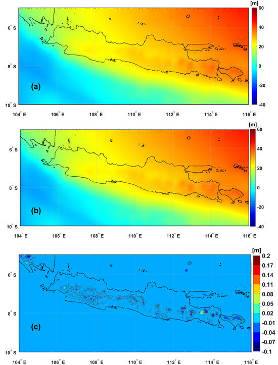
Figure 12.
The result of geoid models and their differences. Geoid model with density (a), geoid model with density (b), and difference between the geoid models with densities and overlaid with topographic height contours at 500 m (c).
This is further seen from the comparison between the and models. The discrepancies between these models range from −12.51 cm to 29.34 cm with a mean of 0.3 cm (note that the relatively small mean difference is possibly arising due to the zero mean removal for each geoid model to eliminate systematic offsets) and a standard deviation of 1.36 cm. As evidence, the minimum and maximum discrepancies between and span from −0.13 to approximately 0.30 m. This range indicates that the impact of using varying density models is non-negligible, especially considering the local geoid height differences, which could significantly affect precise geoid modeling and height determination in particular areas. Therefore, adopting an appropriate density model is crucial for minimizing errors and achieving optimal geoid accuracy. This is likely due to the amplified gravitational effects of dense lithologies and topographic variations in high-relief regions, which are better captured by the lateral density model.
4.4. Geoid Accuracy Assessment
A total of 186 GNSS/leveling points, measured and processed by BIG, were used to validate the results of the gravimetric geoid model. These points were obtained from tidal benchmarks (BMs), starting at the northern coast of Java Island in Semarang and extending to the tidal BM in Glagah, Yogyakarta. The validation route spans a wide range of topographic conditions, beginning at the coastal lowlands in Semarang, crossing through the elevated mountainous regions of central Java, and ending at the southern coast in Yogyakarta (see Figure 1). The geometric geoid undulation values along the validation route range from approximately 25 to 27.5 m. These values, obtained using geometric methods, serve as benchmarks for validating the gravimetric geoid models computed using constant density and the laterally varying UNB_TopoDens model .
Figure 13 illustrates a comparative profile of geoid undulations across the GNSS/leveling stations. The geometric geoid (red line) is plotted alongside the gravimetric geoids derived from the constant density (blue) and variable density (green) models. Additionally, the magenta dashed curve shows the difference between the two gravimetric models −, which was scaled for visibility. The figure demonstrates that both gravimetric models reasonably align with the geometric geoid profile, validating the consistency of the modeling approach.
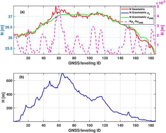
Figure 13.
Comparison of validation results between geometric and gravimetric geoid models. Shown are the geoid models with densities and , and the corresponding validation results (a), and the topographic elevation along the GNSS/leveling validation route (b).
Table 3 further summarizes the statistical discrepancies between the gravimetric and geometric geoid undulations. Both models exhibit nearly identical performance with zero mean error and standard deviations of 10.74 cm for Nc and 10.67 cm for . These results indicate that on average, the choice between constant and laterally varying density models has a minimal effect on model performance along the GNSS/leveling validation line, particularly given that this route primarily traverses moderately elevated terrain.

Table 3.
Statistics of geoid discrepancies between the modeled and geoid heights at validation points.
However, as previously shown in Table 2, the maximum localized geoid differences between and reach up to 30 cm, particularly in regions of high elevation and steep topographical gradients. This reinforces that while overall model statistics may suggest minor improvements, the local impact of lateral density variations can be substantial, potentially affecting high-precision applications such as engineering surveys or vertical datum realization in mountainous areas.
5. Conclusions
We have computed the gravimetric geoid models for Java Island, Indonesia, using the Stokes–Helmert method. Additionally, modeling was conducted using the remove–compute–restore (RCR) technique. Geoid computation involved several processes, including reducing observed gravity to free-air gravity anomalies, smoothing these anomalies to produce Bouguer anomalies, and applying terrain corrections and indirect topography effects. The free-air anomalies were refined through outlier detection and residual gravity anomaly calculation. The Stokes–Helmert method was employed for geoid computation based on a 1D FFT approach to resolve the Stokes function as well as the Stokes function with Wong–Gore modifications. The developed models were then validated using GNSS/leveling data.
Two gravimetric geoid models were developed: one using a constant crustal density ( kg/m3) and another using a variable crustal density model (UNB_TopoDens). Validation against GNSS/leveling data showed that both models achieved similar accuracy, with standard deviations of 10.74 cm and 10.67 cm for the constant and crustal models UNB_TopoDens, respectively. Despite the overall similarity, local geoid differences of up to 30 cm were observed, particularly in regions of significant topographic relief. This highlights that while the average impact of lateral density variations may appear limited, the local effects can be substantial, especially in mountainous or tectonically active zones. These findings support prior studies (e.g., Huang et al. [7]), which demonstrated that incorporating realistic crustal densities can significantly enhance geoid accuracy in complex terrain.
Nevertheless, the study faced limitations, including restricted gravity data distribution and coverage, as well as validation conducted primarily in relatively flat regions (with elevations below 700 m). As such, the results may not fully capture the potential benefits of lateral density modeling in more rugged landscapes. Further, the orthometric height correction implemented to the leveling dataset is still based on a constant density parameter. In the future, density-dependent orthometric corrections should be implemented as performed in prior studies at other locations, e.g., the study by Hwang et al. [49]. Another critical aspect to highlight is the relatively simple methodology used in this study, particularly when computing the topographic corrections. The utilization of more robust computational methods, e.g., using a tesseroid-based approach, as implemented by Lin and Li [11], could further improve the geoid accuracy.
We also stress the importance of extending such investigations to other regions with diverse topographical conditions to systematically evaluate the effects of lateral density variations and better quantify the advantages of incorporating detailed crustal density information in geoid modeling, which a well-distributed GNSS/leveling dataset should support to ensure robust and representative validation. Finally, noticeable data gaps remain over certain land areas, which pose challenges in geoid computation. We acknowledge that more advanced treatments are needed to better handle these gaps, and as part of the future outlook, we plan to implement improved gap-filling techniques and adaptive gridding methods to reduce the impact of incomplete data coverage on geoid modeling.
Author Contributions
Q.G.: investigation, software, formal analysis, writing—original draft, writing—review and editing, visualization. D.D.W.: conceptualization, methodology, formal analysis, investigation, writing—review and editing, supervision. B.B.: conceptualization, methodology, software, formal analysis, investigation, writing—review and editing, supervision. K.P.: formal analysis, methodology, supervision, writing—review and editing. I.M.: formal analysis, supervision, writing—review and editing. R.L.: software, formal analysis and investigation. C.H.: formal analysis, methodology, supervision, writing—review and editing. A.M.P., B.T., R.I.S.M. and A.N.S.: data curation, resources—review. M.I.: formal analysis, writing—review and editing. All authors have read and agreed to the published version of the manuscript.
Funding
This research was supported by the PPMI FITB 2025 program of the Faculty of Earth Sciences and Technology, Institut Teknologi Bandung.
Data Availability Statement
The gravity and GNSS/leveling datasets can be provided upon reasonable request to the Geospatial Information Agency of Indonesia (BIG).
Acknowledgments
We acknowledge the Geospatial Information Agency of Indonesia (BIG) for providing most of the gravity and GNSS/leveling datasets used for this study.
Conflicts of Interest
The authors declare that there are no conflicts of interest.
References
- Hofmann-Wellenhof, B.; Moritz, H. Physical Geodesy; Springer: Vienna, Austria, 2005. [Google Scholar]
- Hinze, W.J. Bouguer reduction density, why 2.67? Geophysics 2003, 68, 1559–1560. [Google Scholar] [CrossRef]
- Nergizci, M.; Abbak, R.A.; Arisoy, M.O. The effect of crustal density heterogeneity on determining gravimetric geoid: Example in Central Anatolia, Türkiye. J. Asian Earth Sci. 2024, 264, 106037. [Google Scholar] [CrossRef]
- Tziavos, I.; Featherstone, W. First results of using digital density data in gravimetric geoid computation in Australia. In Proceedings of the Gravity, Geoid and Geodynamics 2000: GGG2000 IAG International Symposium, Banff, AB, Canada, 31 July–4 August 2000; Springer: Berlin/Heidelberg, Germany, 2002; pp. 335–340. [Google Scholar]
- Tenzer, R.; Vaníček, P. Correction to Helmert’s orthometric height due to actual lateral variation of topographical density. Rev. Bras. Cartogr. 2003. [Google Scholar] [CrossRef]
- Martinec, Z. Effect of lateral density variations of topographical masses in view of improving geoid model accuracy over Canada. In Contract Report for Geodetic Survey of Canada; University of New Brunswick: Fredericton, NB, Canada.
- Huang, J.; Vaníček, P.; Pagiatakis, S.; Brink, W. Effect of topographical density on geoid in the Canadian Rocky Mountains. J. Geod. 2001, 74, 805–815. [Google Scholar] [CrossRef]
- Sjöberg, L.E. The effect on the geoid of lateral topographic density variations. J. Geod. 2004, 78, 34–39. [Google Scholar] [CrossRef]
- Kiamehr, R. The impact of lateral density variation model in the determination of precise gravimetric geoid in mountainous areas: A case study of Iran. Geophys. J. Int. 2006, 167, 521–527. [Google Scholar] [CrossRef]
- Abbak, R.A. Effect of a high-resolution global crustal model on gravimetric geoid determination: A case study in a mountainous region. Stud. Geophys. Geod. 2020, 64, 436–451. [Google Scholar] [CrossRef]
- Lin, M.; Li, X. Impacts of using the rigorous topographic gravity modeling method and lateral density variation model on topographic reductions and geoid modeling: A case study in Colorado, USA. Surv. Geophys. 2022, 43, 1497–1538. [Google Scholar] [CrossRef]
- Lin, M.; Denker, H.; Müller, J. Gravity field modeling using tesseroids with variable density in the vertical direction. Surv. Geophys. 2020, 41, 723–765. [Google Scholar] [CrossRef]
- Laske, G.; Masters, G.; Ma, Z.; Pasyanos, M. Update on CRUST1. 0—A 1-degree global model of Earth’s crust. Geophys. Res. Abstr. 2013, 15, 2658. [Google Scholar]
- Sheng, M.; Shaw, C.; Vaníček, P.; Kingdon, R.; Santos, M.; Foroughi, I. Formulation and validation of a global laterally varying topographical density model. Tectonophysics 2019, 762, 45–60. [Google Scholar] [CrossRef]
- Tiede, C.; Camacho, A.G.; Gerstenecker, C.; Fernández, J.; Suyanto, I. Modeling the density at Merapi volcano area, Indonesia, via the inverse gravimetric problem. Geochem. Geophys. Geosystems 2005, 6, Q09011. [Google Scholar] [CrossRef]
- Hofmann-Wellenhof, B.; Moritz, H. The Java Convergent Margin: Structure, Seismogenesis and Subduction Processes; Geological Society of London: Vienna, Austria, 2011. [Google Scholar] [CrossRef]
- Pahlevi, A.; Pangastuti, D. Indonesian geospatial reference system 2013 and its implementation on positioning. In Proceedings of the FIG Congress, Kuala Lumpur, Malaysia, 16–21 June 2014; Volume 1, p. 12. [Google Scholar]
- Bramanto, B.; Prijatna, K.; Pahlevi, A.M.; Sarsito, D.A.; Dahrin, D.; Erfan, D.V.; Munthaha, R.I.S. Determination of gravity anomalies in Java, Indonesia, from airborne gravity survey. Tao Terr. Atmos. Ocean. Sci. 2021, 32, 7. [Google Scholar] [CrossRef]
- Laxon, S.W.; Giles, K.A.; Ridout, A.L.; Wingham, D.J.; Willatt, R.; Cullen, R.; Kwok, R.; Schweiger, A.; Zhang, J.; Haas, C.; et al. CryoSat-2 estimates of Arctic sea ice thickness and volume. Geophys. Res. Lett. 2013, 40, 732–737. [Google Scholar] [CrossRef]
- Andersen, O.; Knudsen, P. The DTU17 Global Marine Gravity Field: First Validation Results. In Fiducial Reference Measurements for Altimetry, Proceedings of the International Review Workshop on Satellite Altimetry Cal/Val Activities and Applications, Chania, Greece, 23–26 April 2018; Mertikas, S., Pail, R., Eds.; Springer: Berlin/Heidelberg, Germany, 2020. [Google Scholar] [CrossRef]
- Farr, T.G.; Rosen, P.A.; Caro, E.; Crippen, R.; Duren, R.; Hensley, S.; Kobrick, M.; Paller, M.; Rodriguez, E.; Roth, L.; et al. The shuttle radar topography mission. Rev. Geophys. 2007, 45. [Google Scholar] [CrossRef]
- Denker, H. "Evaluation of SRTM3 and GTOPO30 Terrain Data in Germany". In Proceedings of the Gravity, Geoid and Space Missions, Porto, Portugal, 30 August–3 September 2004; Jekeli, C., Bastos, L., Fernandes, J., Eds.; Springer: Berlin/Heidelberg, Germany, 2005; pp. 218–223. [Google Scholar]
- Becker, J.J.; Sandwell., D.T.; Smith, W.H.F.; Braud, J.; Binder, B.; Depner, J.L.; Fabre, D.; Factor, J.; Ingalls, S.; Kim, S.H.; et al. Global bathymetry and elevation data at 30 arc seconds resolution: SRTM30_PLUS. Mar. Geod. 2009, 32, 355–371. [Google Scholar]
- Olson, C.J.; Becker, J.J.S.D. SRTM15_PLUS: Data fusion of Shuttle Radar Topography Mission (SRTM) land topography with measured and estimated seafloor topography. In NCEI Accession 0150537; National Centers for Environmental Information (NCEI): Asheville, NC, USA, 2016. [Google Scholar]
- Tozer, B.; Sandwell, D.T.; Smith, W.H.F.; Olson, C.; Beale, J.R.; Wessel, P. Global bathymetry and topography at 15 arc seconds: SRTM15+. Earth Space Sci. 2019, 6, 1847–1864. [Google Scholar] [CrossRef]
- Tenzer, R.; Chen, W.; Baranov, A.; Bagherbandi, M. Gravity Maps of Antarctic Lithospheric Structure from Remote-Sensing and Seismic Data. Pure Appl. Geophys. 2018, 175, 2181–2203. [Google Scholar] [CrossRef]
- Featherstone, W.; Dentith, M. A geodetic approach to gravity data reduction for geophysics. Comput. Geosci. 1997, 23, 1063–1070. [Google Scholar] [CrossRef]
- Osborne, J.; Overbay, A. The power of outliers (and why researchers should always check for them) Practical Assessment, Research, and Evaluation; University of Massachusetts Amherst Libraries: Amherst, MA, USA, 2004. [Google Scholar]
- Varga, M.; Pitoňák, M.; Novák, P.; Bašić, T. Contribution of GRAV-D airborne gravity to improvement of regional gravimetric geoid modelling in Colorado, USA. J. Geod. 2021, 95, 53. [Google Scholar]
- Christopher, J.; Yang, H.J.; Jay, K. Geoid Determination in South Korea from a Combination of Terrestrial and Airborne Gravity Anomaly Data. J. Geod. 2013. [Google Scholar] [CrossRef]
- Inerbayeva, A. Determination of a Gravimetric Geoid Model of Kazakhstan Using the KTH-Method. Ph.D. Thesis, Royal Institute of Technology (KTH), Stockholm, Sweden, 2010. [Google Scholar]
- Sansò, F.; Sideris, M.G. Geoid Determination: Theory and Methods; Springer Science: Berlin/Heidelberg, Germany, 2013. [Google Scholar]
- Forsberg, R. Terrain effects in geoid model computations.-lectures notes. In ternational school for the determination and use of the geoid model. In International Geoid model Service; DIIAR: Milan, Italy, 1994. [Google Scholar]
- Lestari, R.; Bramanto, B.; Prijatna, K.; Pahlevi, A.M.; Putra, W.; Muntaha, R.I.S.; Ladivanov, F. Local geoid modeling in the central part of Java Indonesia using terrestrial-based gravity observations. Geod. Geodyn. 2023, 14, 231–243. [Google Scholar] [CrossRef]
- Sjöberg, L.E. Topographic effects by the Stokes-Helmert method of geoid and quasi-geoid determinations. J. Geod. 2000, 74, 255–268. [Google Scholar] [CrossRef]
- Hwang, C.; Hsu, H.J.; Featherstone, W.; Cheng, C.C.; Yang, M.; Huang, W.; Wang, C.Y.; Huang, J.F.; Chen, K.H.; Huang, C.H.; et al. New gravimetric-only and hybrid geoid models of Taiwan for height modernisation, cross-island datum connection and airborne LiDAR mapping. J. Geod. 2020, 94, 1–22. [Google Scholar] [CrossRef]
- Moritz, H. Precise Gravimetric Geodesy; Ohio State University: Columbus, OH, USA, 1974. [Google Scholar]
- Hirvonen, R. Statistical Analysis of Gravity Anomalies; Ohio State University Research Foundation Colombus: Columbus, OH, USA, 1962. [Google Scholar]
- Liu, Y.; Lou, L. Unified land-ocean quasi-geoid computation from heterogeneous data sets based on radial basis functions. Remote Sens. 2013, 14, 2022. [Google Scholar] [CrossRef]
- Borghi, A.; Barzaghi, R.; Al-Bayari, O.; Al Madani, S. Centimeter precision geoid model for Jeddah region (Saudi Arabia). Remote Sens. 2020, 12, 2066. [Google Scholar] [CrossRef]
- Forsberg, R. GRAVSOFT. In GRAVSOFT Technical Manual; Technical University of Denmark: Kongens Lyngby, Denmark, 2008. [Google Scholar]
- Vanicek, P.; Kleusberg, A. The Canadian geoid—Stokesian approach. Manuscripta Geodaetica; Springer: Berlin/Heidelberg, Germany, 1987; Volume 12, pp. 86–98. [Google Scholar] [CrossRef]
- Wong, L.; Gore, R. Evaluation of Modifications to Stokes’ Formula. J. Geophys. Res. 1969. [Google Scholar]
- Abbak, R.A.; Goyal, R.; Ustun, A.; Olgun, S. Combined effects of terrain corrections and deterministic modifiers on the Stokes-Helmert geoid over sophisticated topography. Acta Geod. Geophys. 2025, 60, 29–51. [Google Scholar]
- Li, X.; Wang, Y. Comparisons of geoid models over Alaska computed with different Stokes’ kernel modifications. J. Geod. Sci. 2011, 1, 136–142. [Google Scholar] [CrossRef]
- Heiskanen, W.; Moritz, H. Physical Geodesy; W. H. Freeman & Co.: New York, NY, USA, 1967. [Google Scholar]
- Ben-Zion, Y.; Sammis, C.G. Characterization of Fault Zones. Pure Appl. Geophys. 2003, 160, 677–715. [Google Scholar] [CrossRef]
- Forsberg, R.; Fehr, J. Airborne gravity and geoid determination. In Proceedings of the 2nd International Airborne Gravity Conference. International Association of Geodesy, Budapest, Hungary, 10–14 March 1998; pp. 51–60. [Google Scholar]
- Hwang, C.W.; Hsiao, Y.S. Orthometric corrections from leveling, gravity, density and elevation data: A case study in Taiwan. J. Geod. 2003, 77, 279–291. [Google Scholar] [CrossRef]
Disclaimer/Publisher’s Note: The statements, opinions and data contained in all publications are solely those of the individual author(s) and contributor(s) and not of MDPI and/or the editor(s). MDPI and/or the editor(s) disclaim responsibility for any injury to people or property resulting from any ideas, methods, instructions or products referred to in the content. |
© 2025 by the authors. Licensee MDPI, Basel, Switzerland. This article is an open access article distributed under the terms and conditions of the Creative Commons Attribution (CC BY) license (https://creativecommons.org/licenses/by/4.0/).