Dynamics of Water Quality in the Mirim–Patos–Mangueira Coastal Lagoon System with Sentinel-3 OLCI Data

Abstract

The Mirim–Patos–Mangueira coastal lagoon system provides a wide range of ecosystem services. However, its vast territorial extent and the political boundaries that divide it hinder integrated assessments, especially during extreme hydrological events. This study is divided into two parts. First, we assessed the spatial and temporal patterns of water quality in the lagoon system using Sentinel-3/OLCI satellite imagery. Atmospheric correction was performed using ACOLITE, followed by spectral grouping and classification into optical water types (OWTs) using the Sentinel Applications Platform (SNAP). To explore the behavior of water quality parameters across OWTs, Chlorophyll-a and turbidity were estimated using semi-empirical algorithms specifically designed for complex inland and coastal waters. Results showed a gradual increase in mean turbidity from OWT 2 to OWT 6 and a rise in chlorophyll-a from OWT 2 to OWT 4, with a decline at OWT 6. These OWTs correspond, in general terms, to distinct water masses: OWT 2 to clearer waters, OWT 3 and 4 to intermediate/mixed conditions, and OWT 6 to turbid environments. In the second part, we analyzed the response of the Patos Lagoon to flooding in Rio Grande do Sul during an extreme weather event in May 2024. Satellite-derived turbidity estimates were compared with in situ measurements, revealing a systematic underestimation, with a negative bias of 2.6%, a mean relative error of 78%, and a correlation coefficient of 0.85. The findings highlight the utility of OWT classification for tracking changes in water quality and support the use of remote sensing tools to improve environmental monitoring in data-scarce regions, particularly under extreme hydrometeorological conditions.

1. Introduction

Extreme weather events, climate change, and global warming have become increasingly prevalent, impacting ecosystems and water bodies around the world. These changes contribute to alterations in water quality, increased frequency of extreme weather conditions, and shifts in ecological balances [1]. Understanding and adapting to these transformations is crucial for effective environmental management. Within this context, the continuous monitoring of aquatic environments—particularly large and ecologically important systems such as coastal lagoons—becomes a strategic priority.

In southern Brazil, the Patos Lagoon, Mirim Lagoon, and Mangueira Lagoon form the largest interconnected lagoon system in South America [2,3,4]. They play crucial roles in the economic and political development of the region, as well as its cultural and environmental preservation. Therefore, it is critically important to quantitatively characterize and monitor the water quality of these lagoons.

In lagoon systems, chlorophyll and turbidity are key indicators of water quality and play a crucial role in the ecological dynamics and health of aquatic environments [5,6]. Chlorophyll-a, a pigment present in aquatic plants and algae, is widely used as an indicator of primary productivity and phytoplankton biomass in lagoon systems. Its concentration reflects nutrient availability, photosynthetic activity, and the overall ecological condition of the aquatic environment [7]. Turbidity, on the other hand, is associated with the concentration of suspended particles in the water column, influencing light penetration and photosynthetic processes [8]. These parameters are essential for understanding water quality dynamics and can be monitored remotely in coastal lagoons using satellite imagery [9,10,11].

This study aims to investigate the spatial and temporal dynamics of water quality in a coastal lagoon system using satellite remote sensing. It explores how water bodies with different optical characteristics can be identified and monitored over time through classification into various optical water types (OWTs) based on their reflectance characteristics. To better understand how these classes relate to water conditions, the analysis includes the use of chlorophyll-a and turbidity algorithms, not to retrieve precise concentration values, but to explore the relative behavior of these parameters across different OWTs. Finally, the study examines the response of the Patos Lagoon to a major flooding event driven by intense rainfall, providing insight into the effects of extreme hydrological conditions on the lagoon’s optical and ecological dynamics.

2. Materials and Methods

Figure 1 illustrates the methodological workflow employed in this study, from data collection to the analysis of an extreme flood event. Sentinel-3A/B OLCI satellite imagery (Level-1) was processed through atmospheric correction and the derivation of surface reflectance (Level-2). Remote sensing algorithms were then applied to estimate chlorophyll-a concentrations and turbidity, while optical water types (OWTs) were classified using the SNAP tool. Next, water masks and pixel filters were applied to remove edge effects, followed by the overlay of chlorophyll-a, turbidity, and OWT classification layers using randomly distributed sampling points. Finally, the impact of the extreme flood event was assessed by comparing in situ turbidity measurements with satellite-derived turbidity estimates, and by generating turbidity maps and analyzing changes in water optical properties.

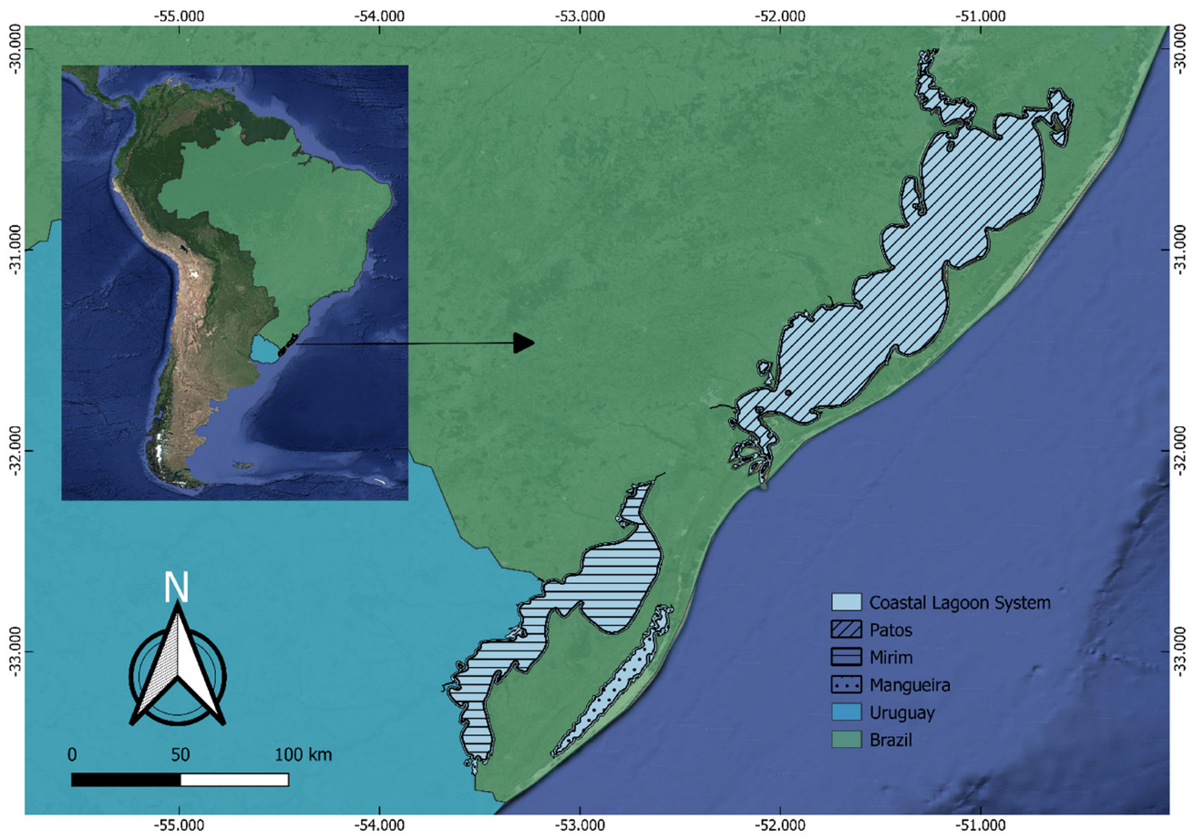
2.1. Study Area

The study area encompasses the Patos–Mirim–Mangueira Lagoon system, located in Brazil and Uruguay (Figure 2). This cross-border region predominantly covers the state of Rio Grande do Sul in Brazil, including the Patos Lagoon (30°30′ S, 51°13′ W to 32°12′ S, 52°05′ W) [12], the Mangueira Lagoon (centered approximately at 33°05′ S, 52°46′ W) [13], and a part of the Mirim Lagoon (32°09′ S, 52°35′ W in Brazil to 33°37′ S, 53°31′ W in Uruguay) [14]. The latter is politically divided into two parts: the larger portion belongs to Brazilian territory, while the remaining area is distributed among the Uruguayan departments of Cerro Largo, Treinta y Tres, and Rocha. Beyond its geopolitical configuration, the system is characterized by distinct hydrodynamic regimes that strongly influence water quality patterns and the applicability of satellite-based monitoring approaches.

This Coastal Lagoon system (CLS) comprises three interconnected coastal lagoons with distinct morphologies and dynamics. The Patos Lagoon, the largest coastal lagoon in the world (~10,360 km²), is shallow (mean depth ~6 m) and connects to the Atlantic Ocean near the city of Rio Grande [15,16]. Its hydrodynamics are influenced by river discharges, especially from the Guaíba, Camaquã, and Capivari rivers [17], as well as wind forcing, tidal intrusion, and seasonal weather events. The lagoon exchanges water with the Mirim Lagoon through the São Gonçalo Channel (~76 km long) [18], with bidirectional flow that depends on rainfall, wind conditions, and water level differences [18].

The Mirim Lagoon (~3749 km²; mean depth ~4.5 m) receives freshwater from several rivers, including the Jaguarão, Arroio Grande, and Cebollatí [19,20]. The São Gonçalo Channel flow is regulated by a lock-dam system to prevent salinization of the Mirim waters during periods of low water level [21]. The Mangueira Lagoon (~820 km²; mean depth ~1.6 m) is a shallow freshwater body directly connected to the Taim wetlands and indirectly to the Mirim Lagoon [21]. Its hydrodynamics are influenced by precipitation, irrigation demands, and wetland connectivity. The entire system is part of the South Atlantic Hydrographic Region and is characterized by strong seasonal variability, shallow morphology, and wind-driven mixing, which together influence the spatial and temporal distribution of water quality and suspended materials.

For the purposes of this study and for convenience, we collectively refer to the Patos Lagoon, Mirim Lagoon, and Mangueira Lagoon as the CLS, acknowledging that these lagoons are sometimes interconnected with each other.

The climate of the CLS is classified as humid subtropical (Cfa, Köppen), characterized by hot summers and relatively cold winters, with mean temperatures ranging from 16 °C to 18 °C, and extremes between −10 °C and 40 °C [22]. The system is influenced by polar, continental, and Atlantic air masses, which shape the region’s weather patterns [22]. Precipitation is well distributed throughout the year, although annual rainfall varies spatially; southern portions of the system (Mirim and Mangueira Lagoons) receive about 1400 mm, while northern areas (Patos Lagoon) receive between 1500 and 1700 mm, with the highest precipitation occurring in the northeast section of the lagoon [22].

2.2. Data Collected

2.2.1. Satellite Images

Considering the large extent of the analyzed territory and the goal of regular monitoring with minimal temporal gaps, the Ocean Land Color Instrument (OLCI) on the Sentinel-3A/B satellites, which provides near-daily global coverage, was chosen as the most suitable sensor [23,24] for our task.

OLCI images were obtained from the European Union’s Copernicus program platform, the Copernicus Data Space Ecosystem (“https://dataspace.copernicus.eu/ (accessed on 12 June 2023)”). OLCI captures data at 21 spectral bands ranging from 400 nm to 1020 nm, with a swath width of 1270 km, and a temporal resolution of ~2 days. The images were acquired as Level 1B products, which include radiometrically and spectrally calibrated top-of-atmosphere (TOA) radiance measurements, expressed in physical units (W·m⁻²·sr⁻¹·µm⁻¹). Each image is georeferenced, and includes geolocation and meteorological metadata and pixel-level classification masks for land, water, and cloud coverage. We used full-resolution (FR) data products, with a spatial resolution of approximately 300 m.

To enhance spatial detail and improve the discrimination of inland and coastal water features.

Thirteen OLCI images were selected to support different parts of the study, each aligned with specific analytical objectives (

Table 1. Summary of the acquisition dates, objectives, and general conditions of the images used.

Acquisition Date	Objective	Cloud Cover (Approx.)	Coastal Lagoon System Condition
13 March 2017	OWT analysis	<10%	Clear
15 October 2017	OWT analysis	<20%	Clear
29 September 2020	OWT analysis	<25%	Clear
30 May 2024	In situ turbidity comparison	<80%	Cloudy overall; sampling pixel clear
20 June 2024	In situ turbidity comparison	<95%	Cloudy overall; sampling pixel clear
30 June 2024	In situ turbidity comparison	<70%	Cloudy overall; sampling pixel clear
1 July 2024	In situ turbidity comparison	<5%	Clear
19 April 2024	Sediment transport	<5%	Clear
6 May 2024	Sediment transport	~50%	Slightly cloudy
9 May 2024	Sediment transport	~50%	Slightly cloudy
14 May 2024	Sediment transport	<75%	Slightly cloudy
2 June 2024	Sediment transport	<40%	Slightly cloudy
2 July 2024	Sediment transport	<10%	Clear

); three images covering a range of optical characteristics were selected for the analysis of OWTs. The first was acquired on 13 March 2017, the second on 15 October 2017, and the third on 29 September 2020. These three cloud-free images were used as a preliminary evaluation of the OWT classification methodology under ideal atmospheric conditions. They served as a baseline to assess the consistency and applicability of the classification in the study area before applying it to the sediment transport analysis on the extreme event case study.

As a case study, for comparison with in situ turbidity data, four images with the lowest cloud cover in the sampling area, acquired on the following dates, were selected: 30 May 2024, 20 June 2024, 30 June 2024, and 1 July 2024. These were the only dates without cloud contamination in the pixels corresponding to the sample collection sites.

For the analysis of sediment transport in the Patos Lagoon, six images were selected to capture the behavior of sediment transport over a three-month period. The images were acquired on the following dates: 19 April 2024, 6 May 2025, 9 May 2024, 14 May 2024, 2 June 2024, and 2 July 2024.

2.2.2. Field Data

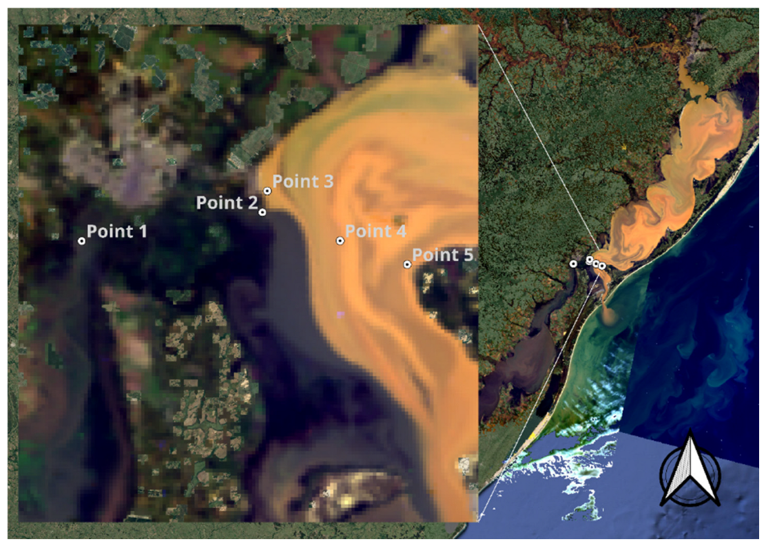
We used in situ measurements of turbidity collected by the “Agência Lagoa Mirim” (ALM). Samples were collected from the surface and analyzed using the nephelometry method, employing equipment with light detectors positioned at 90° from the incident beam. The ALM laboratory ensures the reliability of its analytical procedures. The data were collected at five different sites on four specific dates: 6 April 2024, 18 June 2024, 24 June 2024, and 1 July 2024, resulting in a total of 20 measurements.

These periods coincided with a climatic event of heavy rains and flooding in Rio Grande do Sul. To perform the comparison, we used four OLCI images, acquired on 30 May, 20 June, 30 June, and 1 July 2024. Atmospheric correction was applied using ACOLITE [25]. Turbidity was retrieved using the algorithm from Dogliotti et al. (2015) [26]. For each sample site, a single pixel corresponding to the exact sampling location was extracted to perform a direct one-to-one comparison between in situ and satellite-derived turbidity values. The geographic coordinates (latitude and longitude) of each sampling point are listed in

Table 2. Geographic coordinates (latitude and longitude) of the five sampling points used in this study.

Points	Latitude	Longitude	N° of Samples
Point 1	−31.808692°	−52.385928°	4
Point 2	−31.788555°	−52.225082°	4
Point 3	−31.772344°	−52.220522°	4
Point 4	−31.810787°	−52.156366°	4
Point 5	−31.829354°	−52.096919°	4

.

Four of the sampling locations were in the Patos Lagoon and one was in the São Gonçalo Channel (Figure 3).

In situ measurements of chlorophyll-a concentration were not available for our study area. However, the chlorophyll-a algorithm used in this study, Mishra et al. (2012) [27] is widely recognized for its robustness in highly turbid waters and has been successfully applied in various coastal and estuarine systems. In this study, the algorithm was applied to evaluate the relative distribution of chlorophyll-a across different OWTs, rather than to retrieve precise absolute concentrations.

2.3. Processing of Satellite Imagery Data

Each image was processed using ACOLITE to correct for atmospheric effects [28,29]. ACOLITE corrects for gaseous absorption and molecular scattering using a look-up-table approach based on the 6SV radiative transfer model [30] and aerosol scattering using the dark spectrum filtering method [31]. ACOLITE also corrects for the effects of sun glint and spectral smile, which is a wavelength shift across the spatial axis in the detector due to a change of dispersion angle of the spectral angles with the field position [32]. Sun glint correction is performed by treating observed reflectance in the short-wave infrared (SWIR) bands as a measure of sun glint and extrapolating it to the other bands by using ratios of direct atmospheric transmittance and Fresnel reflectance at the water surface [33]. Spectral smile correction follows the method outlined by Bourg et al. (2008) [34].

Subsequently, at-sensor radiance—the amount of electromagnetic radiation detected by the sensor before any atmospheric correction—was converted to surface reflectance. Reflectance values were generated exclusively for the water pixels (1). This approach helped eliminate land pixels more reliably, ensuring that only valid water pixels were analyzed throughout the study. Finally, glint effects were corrected for each band to produce the FR level 2 product [32,34]. As part of the process, the land and cloud pixels were masked out, retaining only water pixels. ACOLITE yields water-leaving reflectance ($\rho \omega$) in dimensionless units, which were converted to remote sensing reflectance ($Rrs$) as follows:

$$Rrs={\displaystyle \frac{\rho \omega }{\pi }}$$

(1)

Chlorophyll-a concentrations and turbidity were estimated from $Rrs$ using empirical algorithms integrated within the ACOLITE software. Specifically, the algorithm developed by Mishra et al. (2012) [27] was used for chlorophyll-a estimation, while the Dogliotti et al. (2015) [26] algorithm was selected for turbidity retrieval. Results from previous studies have proven the reliability and suitability of these algorithms for inland and coastal waters [29].

2.4. Remote Sensing Chlorophyll-a and Turbidity Algorithms

To examine the relationship between chlorophyll-a and OWTs, we applied the algorithm developed by Mishra et al. [27]. This method is based on the Normalized Difference Chlorophyll Index (NDCI), which uses Rrs at 708 nm and 665 nm, and is expressed as:

$$NDCI={\displaystyle \frac{Rrs\left(708\right) - Rrs\left(665\right)}{Rrs\left(708\right)+Rrs\left(665\right)}}$$

(2)

The NDCI has demonstrated strong performance in highly turbid and optically complex waters, with an overall bias of only around 12% when applied to various coastal and estuarine environments [27]. While the algorithm is frequently used to estimate chlorophyll-a concentrations in lakes and estuaries [27,35,36,37]. In this study, it was employed as a qualitative tool to explore how chlorophyll-a levels vary among different OWT classes. Rather than focusing on accurate retrieval of chlorophyll-a concentration, our objective was to examine variations in chlorophyll-a concentrations across the different OWTs and assess patterns associated with each water type.

To examine turbidity variations across OWTs, we used the Dogliotti et al. [26] algorithm, which has been previously used for estimating turbidity in coastal waters, covering a wide range of turbidity levels [26,38]. The algorithm uses the water-leaving reflectance ($\rho \omega$) at two spectral bands (645 nm and 859 nm) to retrieve turbidity across a wide range of optical conditions. For low-turbidity waters, defined as waters with $\rho \omega$ (645) < 0.05, $\rho \omega$ (645) is used to retrieve turbidity. Waters deemed by this algorithm as low turbidity typically correspond to turbidity levels up to 15 FNU (Formazin Nephelometric Units). For highly turbid waters, defined as $\rho \omega$ (645) > 0.07, $\rho \omega$ (859) is used to retrieve turbidity. For intermediate waters (0.05 < $\rho \omega$ (645) < 0.07), a linear blending of turbidity estimates from both bands is performed using a weighting factor, $\omega$, which increases linearly from 0 to 1 as $\rho \omega$ (645) increases from 0.05 to 0.07. The final turbidity estimate $T$ is computed as follows:

$$T=(1-\omega ) · T_{645}+{\omega ·T}_{859}$$

(3)

where T₆₄₅ and T₈₅₉ represent turbidity values estimated from the 645 nm and 859 nm bands, respectively, using the semi-empirical algorithm described by Nechad et al. (2010) [39]:

$$T_{\lambda }={\displaystyle \frac{A_T·\rho \omega \left(\lambda \right)}{1-\frac{\rho \omega \left(\lambda \right)}{C_T}}}$$

(4)

The calibration coefficients A_T and C_T are wavelength-specific and were obtained from Dogliotti et al. (2015) [26], as shown below in

Table 3. Calibration coefficients A_T and C_T.

$\mathit{\lambda }\left(\mathit{n}\mathit{m}\right)$	AT	CT
645	228.1	0.1641
859	3078.9	0.2112

:

This flexible approach allows reliable turbidity retrieval from satellite data (e.g., MERIS or Sentinel-3/OLCI) in optically complex coastal and estuarine waters. In the context of this study, however, the algorithm was not applied for the purpose of accurate absolute retrieval of turbidity, but rather to explore the relative patterns of turbidity across different OWTs, offering insights into how sediment dynamics vary under distinct optical conditions.

2.5. Optical Water Type Classifier

The OWTs classification was applied to capture and categorize variability in optical properties of water across the lagoon system. While algorithms for chlorophyll-a and turbidity estimation provide quantitative measurements of individual parameters, they may not fully reflect the complex interactions between multiple water constituents—such as suspended sediments, colored dissolved organic matter (CDOM), and phytoplankton—especially in optically complex environments. OWTs serve as a spectral classification framework that groups water pixels based on their reflectance characteristics across different wavelengths. This approach enables a more comprehensive understanding of the optical conditions in the lagoon and supports the interpretation of satellite-derived water quality patterns. Additionally, OWTs can guide the selection or adjustment of algorithms to optimize retrievals based on variations in optical properties of the water body. A single water body may have multiple OWTs, resulting in the adaptive use of different algorithms for retrieving the same parameter from a given water body.

To qualitatively map the lagoon system and distinguish areas with different spectral reflectance behaviors and different OWTs, corrected reflectances are grouped by various classification methods. OWTs were classified using the Sentinel Application Platform (SNAP) software 9.0.0 (“http://step.esa.int/main/toolboxes/snap/ (accessed on 13 February 2024)”) [29,40,41]. The OWT tool is a spectral-based pre-classification system designed to group in situ spectral data into clusters, originally developed by Moore et al. [42]. This approach has been refined to compare remotely sensed water spectra with those collected in the field. Data from various global contributors—including the University of New Hampshire, NASA’s SeaBass (USA), and CEDEX (Spain)—as well as partners of the EU-GLaSS and ESA DUE CoastColour projects, have been incorporated into the tool by the European Space Agency (ESA) [43].

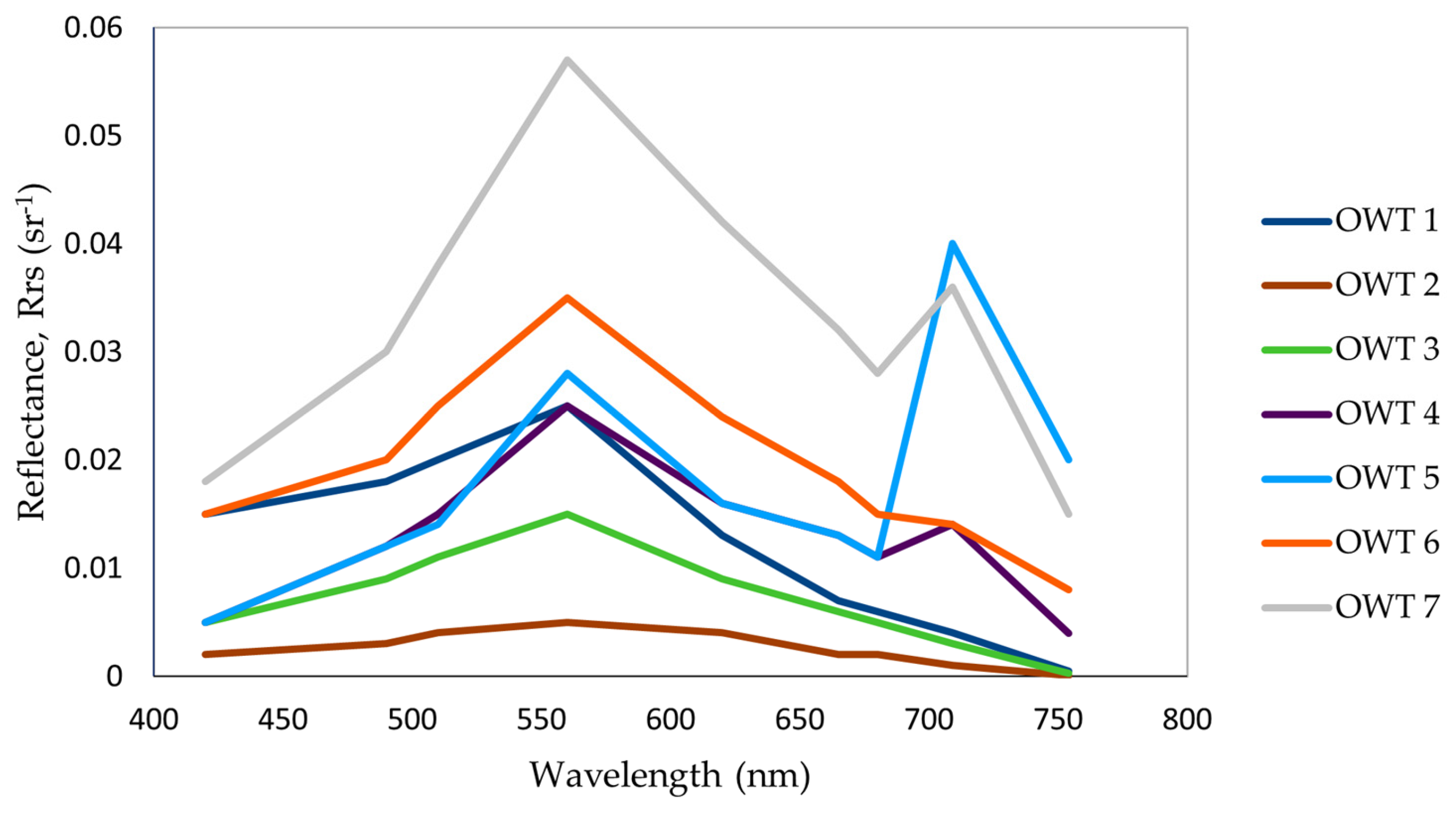
The methodology relies on a fuzzy logic spectral classification model, later adapted for coastal and lake environments [42,44]. For OWT classification, the “Inland no-blue-band” classifier, specifically designed for rivers and lakes, was applied within the SNAP platform. According to the ESA, the OWT classification scheme allows for a maximum of seven clusters, which are not exclusive to any specific water body, geographic region, or water type. Freshwater and marine stations can appear within the same clusters, reflecting similarities in their optical properties rather than strict environmental distinctions. The classification is based on spectral characteristics, particularly absorption patterns in the blue-green region and reflectance variations across key wavelengths.

The ESA OWT classes follow a distinct pattern, wherein classes 1–3 exhibit increasing absorption in the blue and green wavelengths while maintaining low reflectance in the red and near-infrared regions. Classes 4–7, on the other hand, show an increasing peak magnitude at 555 nm. Chlorophyll-a concentration tends to rise from OWT 1 to OWT 5, while OWTs 6 and 7 display lower mean chlorophyll-a values, as detailed in the ESA documentation [43]. The classification process relies on specific Sentinel-3 OLCI wavelengths (490, 510, 560, 620, 665, 680, 709, and 754 nm) to effectively group water bodies based on their optical signatures. This approach provides a robust framework for analyzing water quality dynamics across different aquatic environments, regardless of their freshwater or marine origin. Figure 4 shows the mean reflectance spectra of the seven OWTs used in this study based on the classification scheme developed by the ESA. These spectral patterns form the basis for clustering water bodies according to their optical properties and are used as input for the classification.

2.6. Water Mask and Pixel Filtering

In order to omit land pixels that were not identified by the land mask applied within ACOLITE, we used a water mask created using the Global Surface Water Data Access dataset (“https://global-surface-water.appspot.com/download (accessed on 11 March 2024)”), which provides water occurrence data from 1985 to 2021. This dataset consists of individual tiles measuring 10° × 10°, and for this study, the tile covering 30–40° S and 50–60° W was selected.

The raster file represents the percentage of water occurrence over time for the Patos Lagoon, the Mangueira Lagoon, the Mirim Lagoon, and the São Gonçalo Channel. A binary raster was generated, with a value of 1 assigned to water pixels and 0 to non-water pixels. This water mask was then applied to the chlorophyll-a concentration, turbidity, and OWT results to exclude land pixels remaining after the application of the land mask in ACOLITE.

In addition to applying the water mask, further data processing was performed to refine the chlorophyll-a and turbidity datasets. Pixels with negative chlorophyll-a or turbidity values were removed, along with those affected by clouds that persisted after preprocessing. To enhance image visualization, an RGB composite of the reflectances obtained after preprocessing was also generated.

2.7. Overlaying

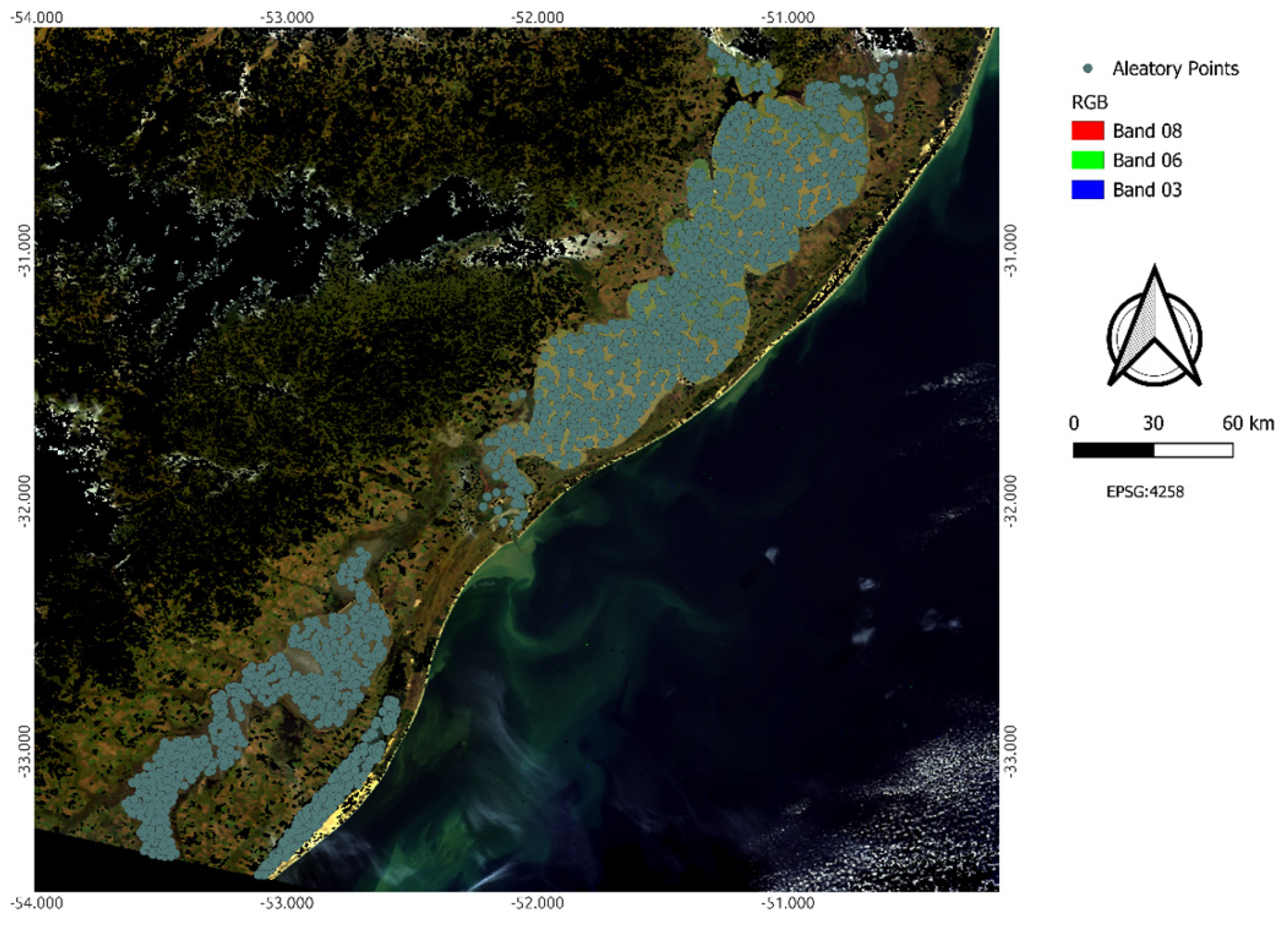
To investigate the relationship between OWTs and water quality indicators, three OLCI images were selected and classified into OWTs. The layers of retrieved chlorophyll-a concentration and turbidity values were overlaid onto the OWT classification, allowing the extraction of average values of chlorophyll-a concentration and turbidity for each OWT. This approach enables the evaluation of the variation of the parameters across the different OWTs and supports the interpretation of water quality dynamics in optically complex environments.

To ensure consistent sampling across the CLS, a layer of 1750 randomly distributed points was generated for each date. The point selection followed three criteria: (1) the points were outside a 1000 m buffer applied along the shoreline to minimize adjacency effects from land; (2) the points were spaced at least 1000 m apart to prevent clustering; and (3) the points were at least two pixels away from cloudy pixels, as manually verified with the true-color composites of corresponding satellite images (Figure 5).

2.8. Statistical Methods

We used a statistical analysis to characterize the water quality parameters for each OWT and assess the differences in water quality across the various OWTs. The statistical analysis began with normality and variance homogeneity tests to assess the distribution of chlorophyll-a and turbidity values across the OWTs.

The Kolmogorov–Smirnov test (n > 50) was used to evaluate normality, where a p-value > 0.05 indicated a normal distribution, while a p-value < 0.05 suggested non-normality. Variance homogeneity was tested using Bartlett’s test, where a p-value > 0.05 suggested equal variances across groups, and a p-value < 0.05 indicated significant differences. If either test rejected the null hypothesis, the Kruskal–Wallis test was applied to determine whether OWTs differed significantly. A p-value < 0.05 in the Kruskal–Wallis test indicated that at least one group was significantly different. In such cases, a post-hoc Dunn test was conducted to identify specific group differences. The Dunn-Q multiple comparison method was used to compute confidence intervals for pairwise differences, with a 95% confidence level applied to identify significantly distinct OWTs.

For the Dunn test, the null hypothesis (H0) is that there is no significant difference between the medians of the compared groups, while the alternative hypothesis (H1) is that there is a significant difference between the medians of the compared groups. The p-value interpretation for this test is as follows: if the p-value < 0.05, the null hypothesis is rejected for the pair of groups i and j, indicating a significant difference between the medians of these groups.

2.9. Validation Metrics: Pearson, Bias, and MAE

For the analysis of the Patos Lagoon, the statistical metrics, Pearson’s coefficient, multiplicative Bias, and multiplicative Mean Absolute Error (MAE) were calculated to evaluate the agreement between turbidity values retrieved from the Sentinel-3/OLCI data and in situ measurements. The Pearson coefficient is defined as:

$$r={\displaystyle \frac{{\sum }_{i=1}^n(X_i-\overline{X})(Y_i-\overline{Y})}{\sqrt{{\sum }_{i=1}^n{{(X}_i-\overline{X})}^2}\sqrt{{\sum }_{i=1}^n{(Y_i-\overline{Y})}^2}}}$$

(5)

where X_i is the value of the predicted variable (model); Y_i is the value of the observed variable (in situ); $\overline{X}$ is the mean of the predicted values; $\overline{Y}$ is the mean of the observed values; and n is the total number of pairs of observations and measurements. Pearson’s coefficient measures the strength and direction of the linear relationship between two variables. It does not measure error, but association [45].

Given that the turbidity data present a highly skewed (non-Gaussian) distribution, span several orders of magnitude (e.g., from 1 NTU to over 1000 NTU), and exhibit heteroscedastic behavior—where measurement error increases proportionally with the observed value—a log10 transformation was applied prior to computing the linear metrics [46].

The multiplicative bias and multiplicative MAE were computed by applying the formulas in log10 space and then back-transforming the results using base-10 These multiplicative metrics are particularly suited for variables like turbidity that exhibit non-Gaussian distributions and heteroscedastic behavior. This approach enables a more meaningful and scale-independent interpretation of model accuracy across a wide range of parameter values. The multiplicative bias was calculated as:

$$Bias={10}^{({\displaystyle \frac{{\sum }_{i=1}^n{log}_{10}\left(M_i\right)-{log}_{10}\left(O_i\right)}{n}})}$$

(6)

where M, O, and n represent the modeled (or estimated) values, observed values, and the number of data pairs, respectively. If Bias = 1, the model is perfect (unbiased); if Bias > 1, the model overestimates; if Bias < 1, the model underestimates. MAE was calculated as:

$$MAE={10}^{({\displaystyle \frac{{\sum }_{i=1}^n\left|\left.{log}_{10}\left(M_i\right)-{log}_{10}\left(O_i\right)\right|\right.}{n}})}$$

(7)

Calculated as a multiplicative quantity, an MAE of 1.0 represents perfect accuracy, whereas an MAE of 1.5 means an average relative error of 50% [46]. This approach allows for a more realistic assessment of model behavior under data conditions commonly observed in aquatic systems like the Patos Lagoon.

3. Results

3.1. Optical Water Types

The classification of OWTs revealed four distinct classes across the study area, each corresponding to different reflectance patterns and optical conditions. Combining the data from all dates revealed that all OWTs were significantly different from each other for both chlorophyll-a and turbidity. The optical water types OWT 1, OWT 5, and OWT 7 were not observed in any of the analyzed dates, indicating that these classes were not present under the optical conditions captured by the selected images during the study period. For OWTs 6, 4, 3, and 2, the mean reflectance profile was calculated across wavelengths, and the standard deviation was added to represent the variability within each OWT. This approach highlights the dominant spectral behavior of each class while also illustrating the internal variability at each wavelength (Figure 6).

On all dates, the chlorophyll-a and turbidity data did not follow normal distributions and exhibited heterogeneous variances. Consequently, the Kruskal–Wallis test was employed, which resulted in a p-value < 0.05 for all three dates, indicating that at least one group is significantly different from the others. This led to the application of the Dunn post-hoc test, which varied for each date.

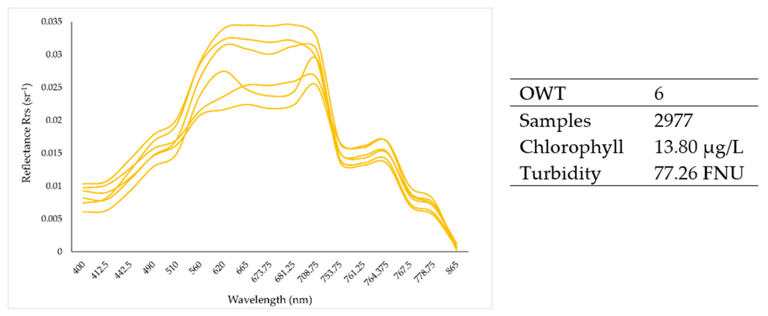
Overall, all OWTs exhibited a reflectance peak near 560 nm, with this peak being most pronounced in OWTs 6, 4, and 3. Additionally, a peak near 708 nm was observed in some of the reflectances spectra from OWTs 6, 4, and 3, and to a lesser extent in OWT 2. Among all reflectances, the OWT 6 had the highest magnitude of reflectance (Figure 7); The reflectance spectra within OWT 6 displayed two different reflectance behaviorspatterns. Thus, one could further sub-divide OWT 6 into two classes. OWT 6 was found primarily in the Patos Lagoon and occasionally in the Mirim Lagoon, and had the highest average turbidity. It was also the most frequently occurring cluster, mainly because most of the pixels from the Patos Lagoon, the largest among the three lagoons, were classified as OWT 6.

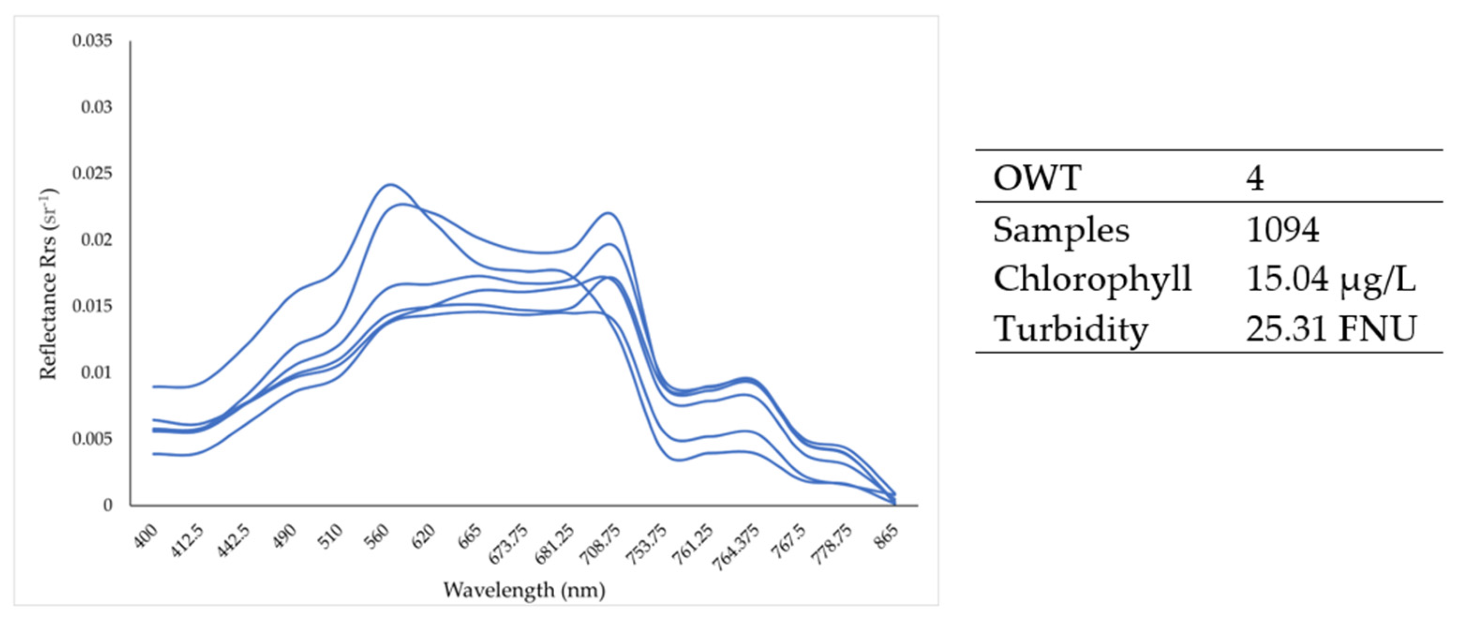
OWT 4 exhibited two distinct reflectance patterns, one with a reflectance peak at 708 nm and the other spectrum exhibiting a spectral shape similar to OWT 3 but with a higher magnitude. OWT 4 had the highest average chlorophyll-a concentrations (Figure 8) and the second highest average turbidity. This cluster was found primarily in the Mirim Lagoon and some in the Casamento Lagoon area in the northern part of the Patos Lagoon. It was also the second largest OWT in terms of spatial coverage as it covered most of the Mirim Lagoon, which is the second largest among the three lagoons, and some of the Patos Lagoon.

OWT 3 demonstrated weak grouping, with two distinct reflectance patterns (Figure 9). Additionally, OWT 3 was found mostly in the Mangueira Lagoon and some in the Patos Lagoon. This cluster also exhibited low average values of both chlorophyll-a and turbidity.

In general, OWTs 3 and 4 had similar reflectance features near 560 nm and 708 nm. However, they differed in the magnitudes of the, reflectance.

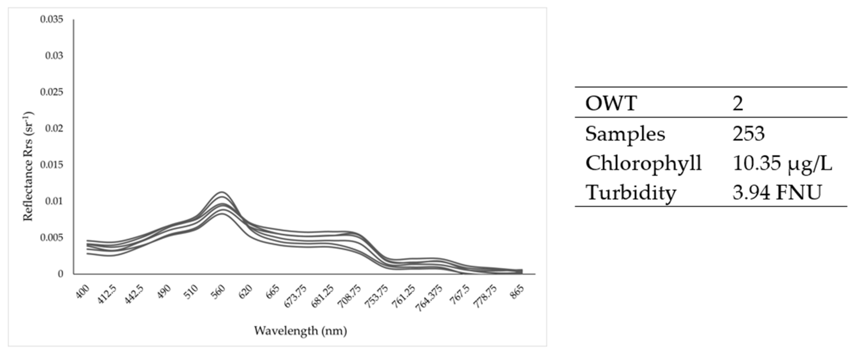
OWT 2 was characterized by low reflectance magnitude and had the lowest average values for of chlorophyll-a and turbidity (Figure 10). OWT 2 was found only in the Mangueira Lagoon, making this lagoon a key area in the study for the characterization of this cluster.

We analyzed the images acquired on 13 Mar 2017, 15 Oct 2017, and 29 Sep 2020 to assess temporal variations in chlorophyll-a concentration and turbidity across the OWTs. The mean values of chlorophyll-a concentration and turbidity were calculated for each OWT, all dates combined and individually for each of the three dates (

Table 4. Date-specific and overall mean chlorophyll-a concentration and turbidity values for each OWT.

OWT	Parameter	All Dates	Date 1 (29 September 2020)	Date 2 (13 March 2017)	Date 3 (15 October 2017)
6	Chl-a (µg/L)	13.80	15.71	15.25	11.39
	Turb. (FNU)	77.26	66.25	90.55	68.59
4	Chl-a (µg/L)	15.04	14.54	17.32	14.42
	Turb. (FNU)	25.31	25.06	30.07	22.09
3	Chl-a (µg/L)	11.62	9.23	15.58	10.83
	Turb. (FNU)	7.76	9.23	7.23	5.45
2	Chl-a (µg/L)	10.35	10.49	9.96	10.31
	Turb. (FNU)	3.94	3.83	4.12	4.50

).

OWTs 2, 3, 4, and 6 were identified in the lagoon system. For the image acquired on 29 September 2020, the average chlorophyll-a concentrations was10.493 μg/L for pixels classified as OWT 2, 9.230 μg/L for OWT 3, 14.544 μg/L for OWT 4, and 15.710 μg/L for OWT 6. Additionally, many chlorophyll-a values in OWT 3 fell outside the boxplot range, and the images were reviewed multiple times to prevent pixel contamination.

Likewise, the average turbidity was 3.83 FNU for OWT 2, 9.23 FNU for OWT 3, 25.06 FNU for OWT 4, and 66.25 FNU for OWT 6. For OWT 3, two distinct spectra, labeled A and B, were identified. Although the classifier grouped the data based on the 709 nm wavelength, reflectance responses in Band 11 varied significantly between A and B. This suggests the need for further refinement of OWTs to better differentiate water types within the lagoon system. 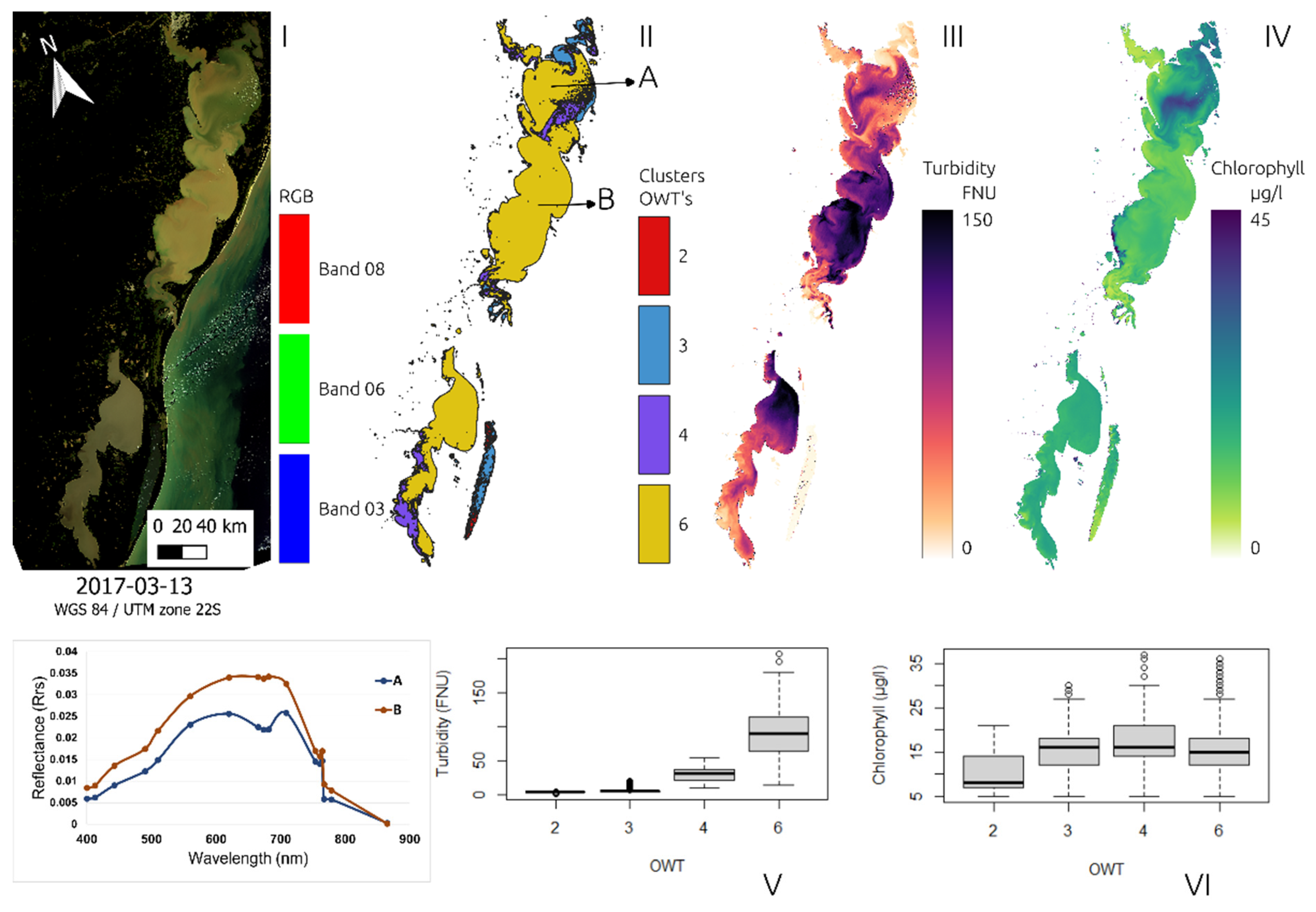In Figure 11I (RGB 8, 6, 3) show a true color composite of the study area from the 29 September 2020 image, the OWT classifications, and the retrieved chlorophyll-a and turbidity values, Figure 11IV shows, high chlorophyll-a concentrations in the middle of the Patos Lagoon due to the presence of an algal bloom.

For the 13 March 2017 image, the average chlorophyll-a concentration was 9.965 μg/L for OWT 2, 15.58 μg/L for OWT 3, 17.32 μg/L for OWT 2, and 15.25 μg/L for OWT 6. Similarly, the average turbidity was 4.123 FNU for OWT 2, 7.23 FNU for OWT 3, 30.07 FNU for OWT 4, and 90.55 FNU for OWT 6. For the different OWTs or water types, some random points were selected to verify reflectance groupings. For OWT 6, two distinct spectra were identified, labeled A and B. In spectrum A, there are two peaks in bands 7 (620 nm) and 11 (708.75 nm), while reflectance decreases in bands 8 (665 nm) and 10 (681.25 nm). In contrast, spectrum B of the same OWT shows an increase in band 7, which plateaus until band 11, where it decreases again (Figure 12).

For the lagoon dataset from 15 October 2017, the average chlorophyll-a concentration was 10.31 μg/L for OWT 2, 10.83 μg/L for OWT 3, 14.42 μg/L for OWT 4, and 11.39 μg/L for OWT 6. Notably, on this date, the chlorophyll-a averages for OWTs 2 and 3 were very similar, suggesting comparable optical conditions between these water types.

Likewise, the average turbidity was 4.50 FNU for OWT 2, 5.45 FNU for OWT 3, 22.09 FNU for OWT 4, and 68.59 FNU for OWT 6. These results indicate that as the OWT number increases, the turbidity average also increases.

As in previous figures, reflectance groupings were analyzed by selecting some random points. Different reflectance behaviors were observed in OWT 4; two spectra with slightly different behavior in band 9 (675 nm) were found. In the figure, reflectances are represented as A and B. This difference might be explained by the classifier not using the 675 nm band, corresponding to band 9 of the OLCI instrument. The number of bands in the OLCI instrument could benefit the creation of OWTs, so this classifier might not be the most suitable for distinguishing OWTs (Figure 13).

3.2. Water Quality Dynamics During the Extreme Flooding Event in 2024

To evaluate the effects of an extreme weather event that occurred in May in Rio Grande do Sul, Sentinel-3/OLCI satellite images were used to analyze the impact of heavy rainfall and the resulting sediment transport. In situ measurements of turbidity provided by the ALM were compared with estimates derived from Sentinel-3/OLCI imagery. A total of 20 sampling points were analyzed.

The Pearson correlation coefficient for these data was 0.85, indicating a strong linear relationship between the satellite-derived turbidity estimates and the in situ measurements, suggesting that the model effectively captures the general trends of variations in turbidity. The multiplicative bias, calculated using Equation (6), was only 0.974 (recall that a multiplicative bias value of 1 signifies no bias), revealing only a slight underestimation, meaning that, on average, the satellite-derived turbidity values were lower than the in situ measurements by approximately 2.6%. The MAE was 1.78, which indicated an average relative error of 78%, which could be attributed to multiple factors, including the temporal interval between the satellite data and in situ measurements, which can have a significant effect in a dynamic environment such as the CLS.

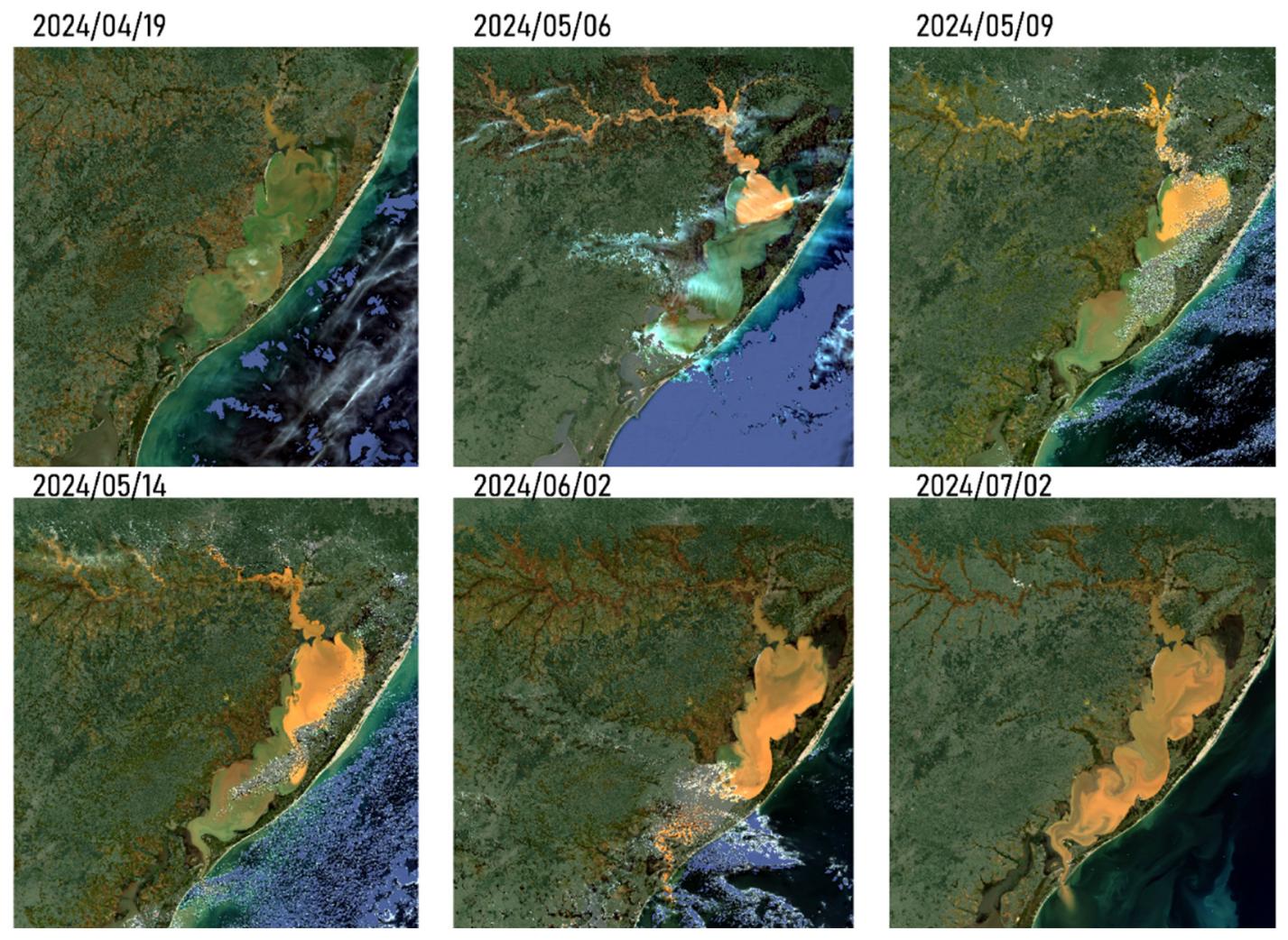
The six satellite images used in this analysis showed distinct spatio-temporal patterns of sediment transport in the Patos Lagoon. The images provided detailed observations, as illustrated in Figure 14, which highlights the six key dates considered in this study to identify sediment movement.

It was observed that the tributaries of the Patos Lagoon exhibit different colors, indicating varying sediment loads. The sediment plumes from the Guaíba and Camaquã rivers showed well-defined dynamics, with the plume from the Guaíba River shown moving through the lagoon in successive images. The images also revealed an increase in the plume size in the São Gonçalo channel from April to July.

In Figure 14, 2024/04/19, the Patos Lagoon exhibited a typical sediment load. However, by 2024/05/06, eight days after the onset of the severe weather event in Rio Grande do Sul (which began on April 28), water levels had risen, and Sentinel-3/OLCI captured high discharge levels from the Guaíba river and substantial sediment loads from the tributaries.

On 9 May 2024 (2024/05/09), the plume advanced toward the sea, following a path along the right margin. By 14 May 2024 (2024/05/14), linear features of sediments had formed in the southern part of the lagoon, influenced by the wind and influx of varying sediment concentrations from tributaries. On 2 July 2024 (2024/07/02), these linear features appeared well-defined, likely due to limited transverse mixing.

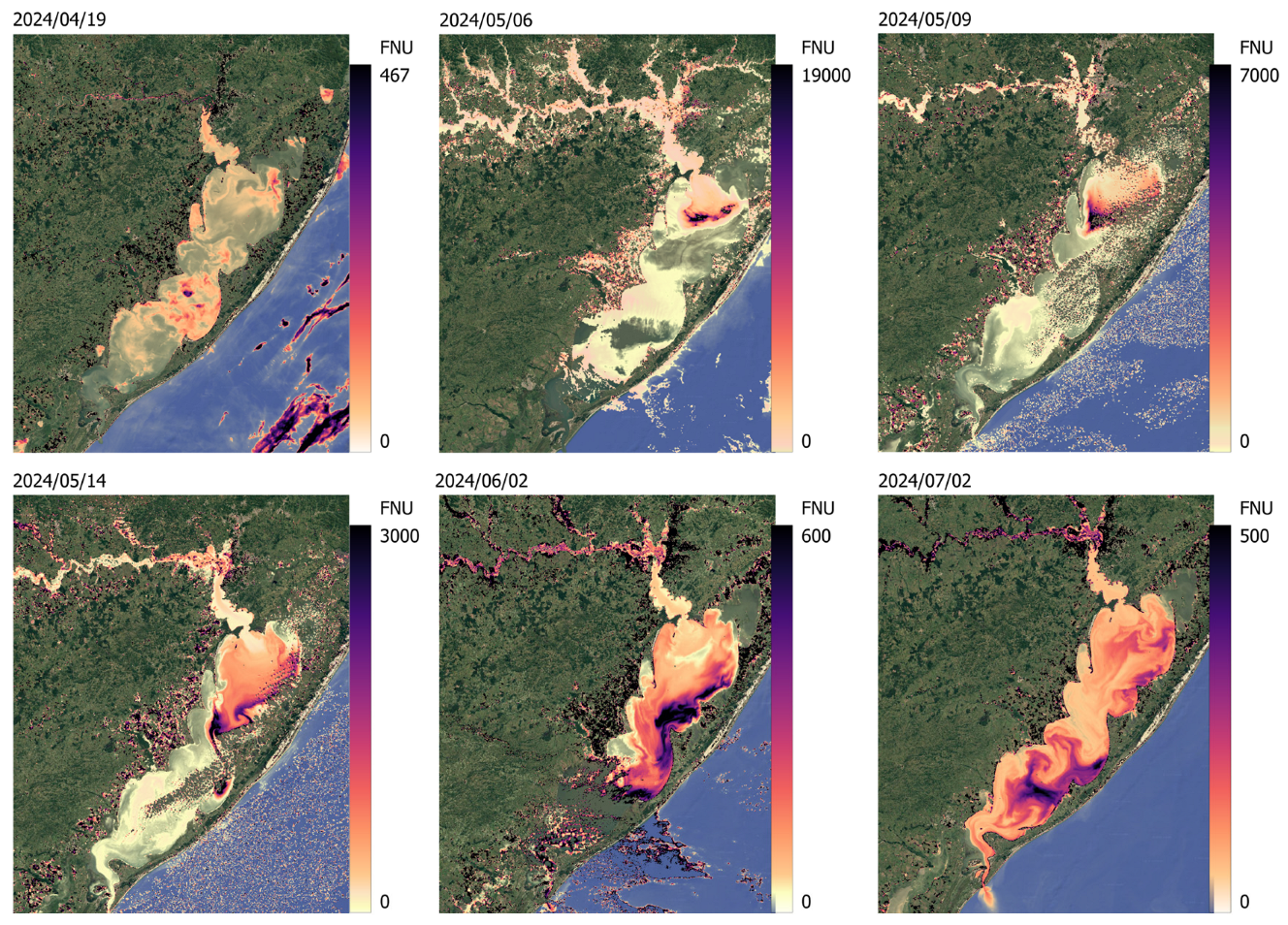
After atmospheric correction, turbidity values retrieved through the Dogliotti et al. (2015) algorithm showed seasonal variations across the six dates, with the maximum retrieved turbidity being 467 FNU for 2024/04/19, 19625 FNU for 2024/05/06, 7032 FNU for 2024/05/09, 3003 FNU for 2024/05/14, 611 FNU for 2024/06/02, and 517 for 2024/07/02.turbidity products were generated using the algorithm from Dogliotti, which highlighted the sediment plume from the Guaíba tributary river and its path through the lagoon, as shown in Figure 15.

The turbidity concentrations observed in the northernmost part of the Patos Lagoon, particularly in the Casamento Lagoon, remained relatively stable, ranging from 4.65 FNU to 12.34 FNU across the period from April to July 2024. This limited variation suggests that this region may be less responsive to precipitation-driven sediment inputs, potentially due to localized hydrodynamic conditions, reduced fluvial influence, or geomorphological features that buffer it from broader sediment dispersion processes. Additionally, the low renewal rate observed in this area, with minimal external inputs and limited circulation, further contributes to somewhat stable levels of turbidity. These factors indicate that, even during high precipitation events, sediment dynamics in this particular region within the lagoon are largely unaffected due to hydrodynamic isolation.

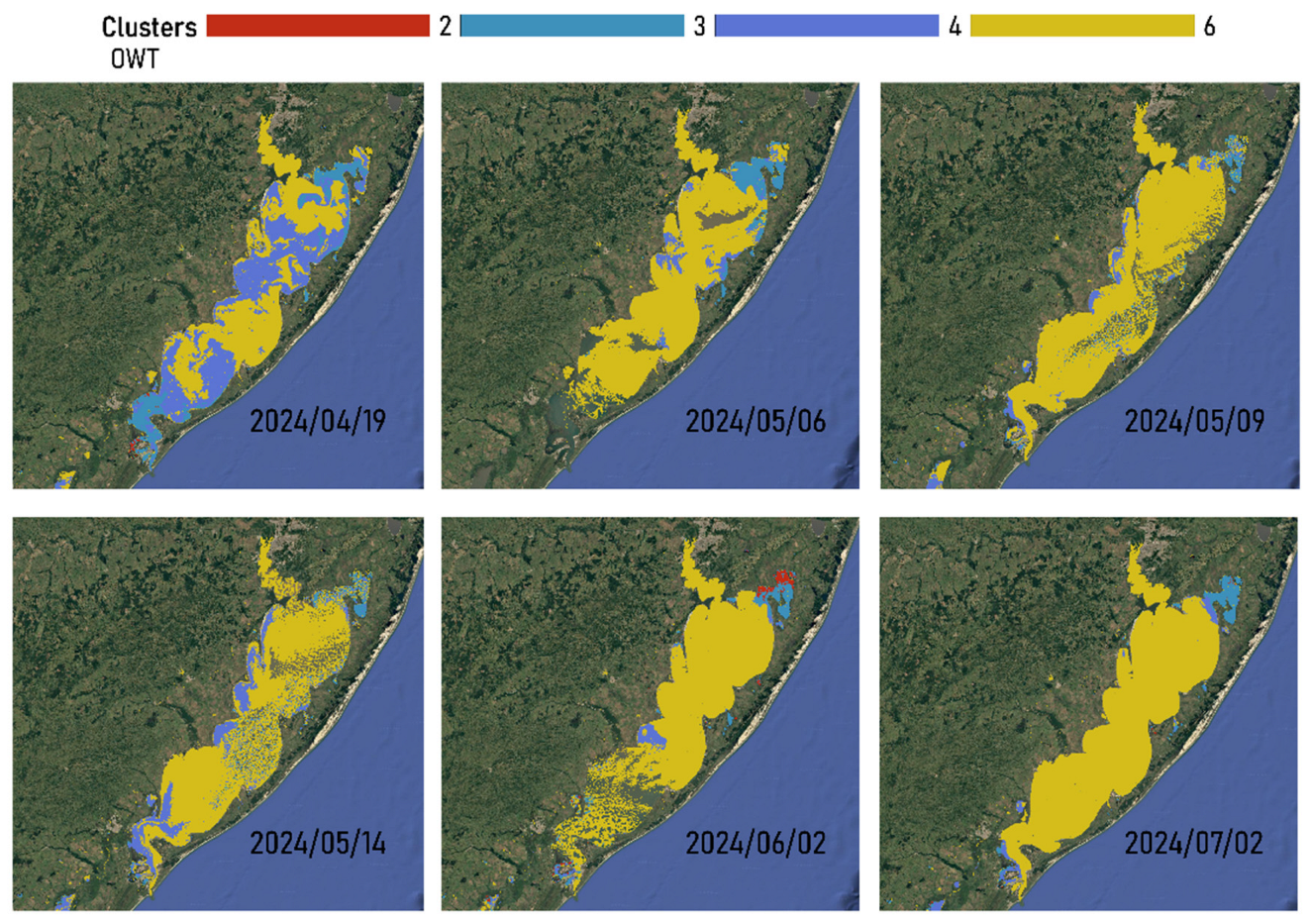
In order to further explore the sediment dynamics within the Patos Lagoon, we determined the OWTs for each of the six images. This provided insight into the influence of turbidity and sediment transport on OWT classification.

The results showed that OWT 6 was the most prevalent water type (Figure 16), which is associated with elevated turbidity due to high suspended sediment concentrations. As shown in previous results, OWT 6 corresponds to the cluster with the highest average turbidity values.

OWTs 2, 3, and, to a lesser extent, OWT 4 were present in the extreme northeastern region of the lagoon, particularly in the Casamento Lagoon. These water types have low particle concentrations characteristic of relatively clean inland waters and were associated with the lowest average turbidity values.

4. Discussion

Reflectance spectra further elucidated these relationships. A peak at 560—common across all spectra—indicates increased scattering due to both organic (e.g., phytoplankton) and inorganic (e.g., sediment) particles [44]. OWT 6 presented two spectral behaviors, both associated with suspended material [10]; one reflecting turbid waters dominated by sediments [47,48], and the other representing non-algal particles typical of estuarine or riverine inflows [49]. The line for OWT 6 represents high turbidity with relatively low TSM concentrations, confirming earlier classifications [47].

OWT 4 also displayed dual spectral behaviors. One spectrum suggests highly productive inland waters with a peak at 709 nm—an indicator of high chlorophyll-a concentration and phytoplankton biomass [47,48]. The other resembles OWT 3, but with higher total suspended matter concentrations [47]. Similarly, OWT 3 included two distinct spectra, one representing clean inland waters [47] and another indicative of productive waters with phytoplankton dominance [47,50]. Despite some spectral overlap, OWTs 3 and 4 differ in spectral magnitudes, suggesting differences in light fields, which may be influenced by particle size and composition [42].

OWT 2 was the most distinct, with consistent spectral grouping and low reflectance values, characteristic of clean or clear inland waters [48,49,50,51]. These findings are supported by prior studies identifying OWT 2 as a low-particulate water concentration and low reflectance magnitude [44,50].

The behavior of OWTs observed across different dates revealed distinct patterns of chlorophyll-a and turbidity concentrations, highlighting the complex dynamics of water quality in the Patos Lagoon. On 29 September 2020, the results do not align with findings reported in other studies on chlorophyll-a and water types with different algorithms [41,44,50,52]. For turbidity, however, values increased progressively with higher OWT classes, showing an exponential rise from OWT 2 to OWT 6. This trend suggests a possible correlation between higher total suspended matter and increasing OWT classes [50].

On 13 March 2017, a different chlorophyll-a pattern was observed; there was a gradual increase in the average chlorophyll-a concentrations from OWT 2 to OWT 4, followed by a decrease in OWT 6. This pattern is consistent with findings from other studies using alternative algorithms [44,50]. Turbidity concentrations, again, showed an exponential increase from OWT 2 to OWT 6, reinforcing the link between higher OWT classifications and total suspended matter [50]. A similar pattern was observed on 15 October 2017, where both chlorophyll-a and turbidity trends aligned with findings from Eleveld et al. [50].

The results of this study highlight the need to adjust the algorithms used to estimate chlorophyll-a and turbidity through remote sensing, as well as to expand the analysis of OWTs, given that this research area is still under development. The guidelines and applications of OWT classification schemes are still being explored, reinforcing the importance of testing complementary approaches. The classification performed using the SNAP tool and the “Inland no-blue-band” classifier with Sentinel-3/OLCI data did not detect all OWTs present in the lagoon system, such as green waters associated with microalgae blooms, which were expected on 29 September 2020, in the Patos Lagoon. Therefore, it is suggested that different classifiers be evaluated for this region.

Beyond the spectral and OWT patterns, this study also aligns with research that links sediment distribution to hydrodynamic and meteorological conditions in the Patos Lagoon. Previous works have reported increased organic matter and sediment plumes during high precipitation events [12]. The sediment flows from these tributaries are interdependent with the broader sediment dynamics of the Patos Lagoon, as also noted in earlier research [53]. The extreme flood event that occurred in May 2024 had a significant impact on the hydrodynamic behavior of the Patos Lagoon system. Rainfall accumulation in the upstream regions reached exceptional levels, with some municipalities in Rio Grande do Sul, such as Caxias do Sul (707.2 mm), Soledade (635.4 mm), and Serafina Corrêa (634.8 mm), registering over 500 mm of precipitation in just the first 13 days of the month, when the monthly climatological average for these municipalities does not exceed 153 mm in May [54]. This intense rainfall caused substantial increases in Guaíba river discharge, principally, and inflow to the lagoon, altering circulation patterns and sediment transport routes.

The behavior of the Guaíba river plume and the formation of current lines observed in this study align with earlier findings describing its interaction with the submerged barrier [55]. The seaward movement along the right margin, noted on 9 May 2024, reflects patterns previously documented under similar hydrodynamic conditions [56]. Furthermore, the well-formed current lines observed on 2 July 2024 correspond to modeled scenarios of the Patos Lagoon, where low transverse mixing plays a significant role [55,57].

The analyzed dates overall revealed sediment load behaviors consistent with the conceptual model previously developed to represent the typical dynamics of suspended particulate matter during periods of high input [15]. This alignment suggests that, under elevated discharge conditions, the transport and distribution of sediments in the Patos Lagoon follow predictable patterns, reinforcing the applicability of the conceptual framework to real-world scenarios observed during the study period.

Although previous studies have shown that high precipitation events typically result in widespread sediment plumes and increased turbidity across the Patos Lagoon [15], the findings of this study suggest that turbidity distribution is not uniform throughout the system.

In particular, the northernmost region of the Patos Lagoon, especially the Casamento Lagoon, exhibited limited turbidity variability, consistent with results from the Eulerian transport models developed using SisBaHiA [16], which show that during the winter season—when the analyzed precipitation event took place—this region experiences the lowest water renewal rates in the lagoon. After 90 days of simulation, the renewal rate reached only 68%, and the water age was estimated at 52 days, classifying it as the oldest water mass in the lagoon [16].

To further support the low water renewal rates observed in the northern portion of the Patos Lagoon during the flood period, meteorological data from a nearby weather station were analyzed. In winter, the predominant wind direction is from the northeast (NE), with approximately 31% of wind events coming from that sector. Wind speeds typically range between 2 and 6 m/s, with some episodes exceeding 6 m/s [58]. These NE winds drive surface water toward the southwestern part of the lagoon, potentially restricting the inflow and circulation in the northern arms, such as the Casamento Lagoon. This wind-induced hydrodynamic pattern helps explain the limited turbidity variability and the long water residence times (over 50 days) previously reported by Eulerian transport models for this region. The combination of low renewal, persistent wind forcing, and morphological enclosure supports the classification of this sector as hosting the oldest water mass in the lagoon during the study period.

Although the OWTs classification proved useful for distinguishing water masses under typical conditions, its performance was notably limited during the extreme weather event of May 2024. This limitation can be attributed primarily to the unusually high cloud cover throughout the three-month analysis period. The unprecedented volume of rainfall led to persistent cloud formation and saturation in the region, severely reducing the availability of cloud-free pixels. As a result, even after careful filtering and selection, many of the remaining satellite scenes still contained contaminated pixels with anomalously high reflectance values due to thin clouds or cloud shadows. These compromised pixels likely interfered with the classification process, resulting in the misclassification or underrepresentation of certain water types. Consequently, the ESA OWT classifier did not accurately reflect the optical complexity of the lagoon during this event, particularly failing to capture water masses associated with flood-driven processes. This underscores the importance of integrating improved cloud masking techniques and complementary classification methods for monitoring during extreme hydrometeorological conditions.

Despite these limitations, OWT classification proved to be a useful tool for providing spatial information about the southern coastal lagoon system, contributing to the understanding of the distribution and long-term trends of water optical states. Moreover, these classifications can serve as intermediate products to enhance the selection of algorithms for retrieving water quality parameters. Thus, the data generated through this approach has the potential to support water resource management and water quality assessments, contributing to decision-making aimed at preserving and sustainably using regional aquatic ecosystems.