Article

Can Combining Machine Learning Techniques and Remote Sensing Data Improve the Accuracy of Aboveground Biomass Estimations in Temperate Forests of Central Mexico?

by
Martin Enrique Romero-Sanchez
*,
Antonio Gonzalez-Hernandez
,
Efraín Velasco-Bautista
,
Arian Correa-Diaz
,
Alma Delia Ortiz-Reyes
and
Ramiro Perez-Miranda
National Institute of Forestry, Agriculture and Livestock Research, Mexico City 04010, Mexico
*
Author to whom correspondence should be addressed.
Geomatics 2025, 5(3), 30; https://doi.org/10.3390/geomatics5030030
Submission received: 21 May 2025 / Revised: 25 June 2025 / Accepted: 2 July 2025 / Published: 3 July 2025

Abstract

Estimating aboveground biomass (AGB) is crucial for understanding the carbon cycle in terrestrial ecosystems, particularly within the context of climate change. Therefore, it is essential to research and compare different methods of AGB estimation to achieve acceptable accuracy. This study modelled AGB in temperate forests of central Mexico using active and passive remote sensing data combined with machine learning techniques (Random Forest and XGBoost) and compared the estimations against a traditional method, such as linear regression. The main goal was to evaluate the performance of machine learning techniques against linear regression in AGB estimation and then validate against an independent forest inventory database. The models obtained acceptable performance in all cases, but the machine learning algorithm Random Forest outperformed (R2cv = 0.54; RMSEcv = 19.17) the regression method (R2cv = 0.41; RMSEcv = 25.76). The variables that made significant contributions, in both Random Forest and XGBoost modelling, were NDVI, kNDVI (Landsat OLI sensor), and the HV polarisation from ALOS-Palsar. For validation, the Machine learning ensemble had a higher Spearman correlation (r = 0.68) than the linear regression (r = 0.50). These findings highlight the potential of integrating machine learning techniques with remote sensing data to improve the reliability of AGB estimation in temperate forests.

1. Introduction

Temperate forests are a vital component of the global ecosystem, providing crucial ecosystem services such as carbon sequestration, water regulation, and habitat preservation [1]. These forests are characterised by distinct vertical stratification, with an understory layer comprising shrubs, herbs, and ferns, each contributing to the overall biodiversity and ecosystem functioning. They are composed of diverse tree species, including deciduous and evergreen varieties, which are crucial in storing aboveground carbon through biomass accumulation [2]. Managed temperate forests have garnered significant attention in climate change mitigation, as they can enhance carbon sequestration through sustainable management practices [3,4,5].
Accurate aboveground biomass (AGB) estimation is crucial for sustainable forest management and climate change mitigation efforts [6]. Conventional approaches to biomass estimation, such as field-based measurements and applying allometric models, often exhibit spatial, attributional, and temporal gaps [6]. Traditional field-based methods can be time-consuming, labour-intensive, expensive, and limited in spatial coverage. Therefore, remote sensing techniques have been explored as a more efficient and cost-effective alternative [7,8]. Remote sensing techniques have become increasingly crucial in environmental monitoring and natural resource management, particularly in estimating aboveground biomass, which is a vital indicator of ecosystem health, carbon sequestration, and the overall productivity of terrestrial ecosystems [9]. However, biomass estimation accuracy is often constrained by the spatial resolution of the remote sensing, which can be particularly problematic when dealing with heterogeneous or complex forest structures [10]. Furthermore, the relationship between remote sensing signals and aboveground biomass can be influenced by various factors, such as soil properties, climate, forest species composition, and forest age, requiring careful calibration and validation [11]. Another limitation of remote sensing techniques for biomass estimation is the transferability of the developed models across different geographical regions and periods. Empirical relationships between remote sensing-derived indices and field-measured biomass often exhibit poor transferability, posing a challenge to the broader application of these methods [12].
To address these limitations, ongoing research is focused on improving remote sensing techniques, developing a more robust statistical approach, and integrating multi-source remote sensing data to enhance the accuracy and reliability of AGB estimation. Recent advancements in remote sensing technology and machine learning techniques offer a promising alternative for large-scale biomass estimation [13,14].
Machine learning algorithms have become indispensable tools for estimating forest aboveground biomass using remote sensing data, offering powerful capabilities for handling complex datasets and extracting meaningful relationships between spectral information and forest characteristics [15,16]. Among the machine learning techniques available, Random Forest and XGBoost have emerged as popular and effective methods for biomass estimation, demonstrating strong predictive performance and robustness across diverse forest ecosystems [17]. The utilisation of remote sensing imagery, spanning various spatial and temporal resolutions, presents significant advantages for non-destructive forest biomass monitoring at different scales, which plays a crucial role in addressing ecological issues and understanding small-scale processes [10]. Remote sensing techniques offer a cost-effective and time-efficient means of assessing forest biomass over large areas compared to traditional field-based methods, which are often labour-intensive and limited in spatial coverage [18]. Combining remote sensing data with machine learning algorithms enables the development of accurate and spatially explicit biomass predictions, essential for carbon accounting, forest management, and biodiversity conservation [19,20].
Therefore, in this research, we employed two machine learning algorithms, Random Forests and XGBoost (Extreme Gradient Boosting), and hypothesised that their application to aboveground biomass estimations over temperate forests improves the estimations made by other traditional methods (i.e., linear regression). Also, another hypothesis suggests that combining data from different types (e.g., active and passive) enhances the accuracy of aboveground biomass estimations.

2. Materials and Methods
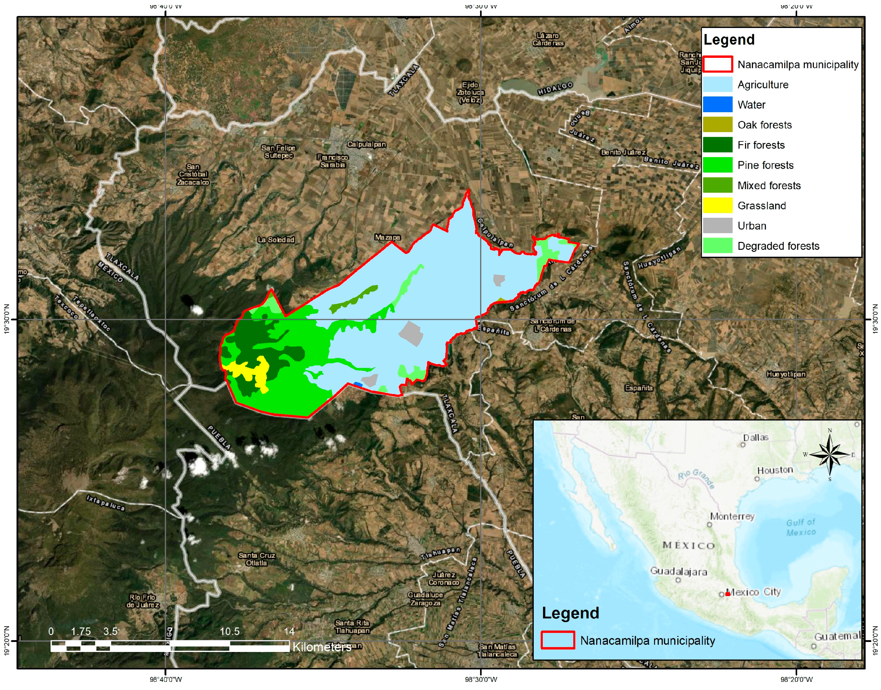
2.1. Study Area

The study area is in the municipality of Nanacamilpa, Tlaxcala, Mexico, between the 19°27′ and 19°34′ north latitude; the meridians −98°26′ and −98°38′ west longitude; altitude between 2600 and 3300 m and it is located within the region known as the Sierra Nevada (19.51° N and −98.65° W). The climate of the study area is temperate sub-humid climates with summer rains, annual precipitation typically 700–1500 mm, and cool summers (~16–20 °C) [2]. The forests of Nanacamilpa, Tlaxcala are considered priority areas for bird conservation, especially for endemic or at-risk species, but are threatened by anthropogenic pressure. The dominant vegetation is coniferous forests made up mainly of pines (Pinus montezumae, P. teocote and P. pseudostrobus), and sacred fir (Abies religiosa Kunth Schltdl. et. Cham.) predominates, growing primarily in the canyons. In contrast, pines, oaks, and cedars are dominant on the hillsides. There are relics of madrone trees (Arbutus xalapensis Kunth) and alder (Alnus firmifolia Fernald). The study area spans approximately 10,018 ha, but the forest area within it is around 2500 ha (Figure 1).

2.2. Forest Inventory Data

2.2.1. Forest Samples

We conducted a forest inventory during the 2020–2021 period and evaluated 82 sampling plots randomly distributed in the study area (square plots of 20 × 20 m, 400 m2). For the establishment and collection of the data, we followed the guidelines from the National Forestry and Soils Inventory databases [21] (INFyS, National Forestry Commission, CONAFOR-Mexico) (Figure 2).
Additionally, during 2021 and 2022, we established eleven 100 × 100 m (1 ha) plots in the Nanacamilpa forests. These plots were numbered consecutively from 1 to 12. Plots numbered 1, 2, 3, 11, and 12 were located within fir forests, whereas the rest of the plots were situated in pine forests with varying levels of management. We measured all trees within these plots and recorded their Diameter at breast height (DBH), height (H), and species names. The idea was to construct an independent database for assessing accuracy, assuming spatial correspondence between the aboveground biomass calculated inside the 1 ha plots and the remote sensing data (Figure 2) [22].

2.2.2. Aboveground Biomass Estimations

The DBH, H, and species name were extracted from each sampling plot and used for calculating individual tree AGB. We used different allometric models for each species (Table 1).
Table 1. This study used allometric models for individual tree aboveground biomass (AGB).
Allometric ModelSpeciesSource
A G B = 0.0713 × D B H 2.5104 Abies religiosa (Kunth) Schltdl. et. Cham.[23]
A G B = 0.0130 × D B H 3.0464 Pinus montezumae Lamb.[24]
A G B = 0.0345 × D B H 2.9334 Quercus sp.[25]
A G B = 0.3764 × D B H 2 ( 2.3146 × D B H ) 1.9106 : Arbutus xalapensis Kunth and Alnus firmifolia Fernald[26]
Individual AGB data (trees) were added on a per-plot basis and used to extrapolate to a per-hectare basis using the “Ratio of Means” [27].

2.3. Remote Sensing Data

2.3.1. ALOS PALSAR

The ALOS (Advanced Land Observing Satellite) PALSAR (Phased Array type L-band Synthetic Aperture Radar) system is a versatile remote sensing technology widely used for various geospatial applications, including biomass estimation. We downloaded ALOS PALSAR mission data from the Google Earth Engine platform, focusing on Level 2 processing imagery for the years 2020–2021. Level 2 data is derived from the raw Level 1 data through processing steps, including radiometric calibration, terrain correction, and geocoding [28]. This processing ensures that the data is georeferenced and that the backscatter values are corrected for terrain and incidence angle factors. However, the data is in digital numbers (DNs), so we transform them to Decibels (dB) using the following equation [29]:
γ0 = 10log10(DN2) − 83.0 dB
Decibels (dB) are a logarithmic unit that expresses the ratio of two values. They are commonly used in the analysis of radar data because they provide a more intuitive representation of the backscatter signal [30]. Then, we performed a speckle filter (a Lee filter with a window size of 3 × 3) to reduce speckle noise without sacrificing the image structure [31]. Later, we obtained images with polarisation HH and HV. The bands HH-HV and HH+HV were derived in the ArcGIS desktop Version 10.8.2 environment through the raster calculators.

2.3.2. Sentinel-1

Sentinel-1 is a synthetic aperture radar (SAR) satellite mission operated by the European Space Agency (ESA). It provides high-resolution imagery that can be used for various purposes, including land cover mapping, natural disaster monitoring, and environmental change detection [32]. We acquired raw Sentinel-1 data from the Copernicus Open Access Hub [33]. Due to the availability and consistency of the imagery, we selected 45 images from the year 2022. Once the images were downloaded, we pre-processed them to correct for various factors that can introduce distortions, such as atmospheric effects, sensor geometry, and radiometric calibration [34]. To convert the Sentinel-1 data to decibels, the following formula was used [33]:
γ0 = 10log10(DN2)
where DN represents the digital number or pixel value in the Sentinel-1 image. All Sentinel-1 processes were carried out under the Sentinel Application Platform (SNAP) environment.
Finally, we computed the mean of all filtered images based on the AOI, date, and polarisation. The result is an image that represents the average backscatter over the specified time (2022) for each of the two polarisations (VH and VV).

2.3.3. Landsat OLI

We used a Landsat 8 Operational Land Imager (OLI) surface image with Level 2 processing, which includes various radiometric and geometric corrections [35]. For consistency purposes, we searched for all Landsat images available in 2022, with less than 10% of clouds. Later, we calculated the median to obtain an image representing the reflectance of the study area. For analysis purposes, we calculated the Normalised Difference Vegetation Index (NDVI) [36], Soil Adjusted Vegetation Index (SAVI) [37], Enhanced Vegetation Index (EVI) [38], Normalised Difference Water Index (NDWI) [39], and the Kernel NDVI (KNDVI) [40], which has been highlighted for its convenience in monitoring terrestrial ecosystems [41].
k N D V I = t a n h ( ( N I R R e d 2 σ ) 2 )
where σ is a length-scale parameter specified in each application and represents the index’s sensitivity to sparsely/densely vegetated regions; a reasonable choice is to take the average value σ = 0.5(NIR + red). NIR is the Near Infrared band.

2.4. Modelling Spatial AGB

To estimate AGB, we constructed a database with the forest inventory’s aboveground biomass values and the corresponding remote sensing data values from ALOS PALSAR, Sentinel-1, and Landsat OLI. We extracted the pixel values from each dataset and stored them as a CSV file for further analysis. We used two machine learning models to model aboveground biomass, but we also performed a linear regression approach for comparison purposes.
Before the AGB modelling, we conducted a Pearson correlation analysis to evaluate and select the best variables derived from the remote sensing data (Table 2). This step ensured efficiency during the modelling process and avoided redundancy.
For correspondence purposes, all images were resampled to the spatial resolution of the Landsat OLI sensor using the Nearest Neighbour method and registered to the same extent. All the spatial analyses were performed inside the ArcGIS Desktop Version 10.8.2 environment. The modelling process was implemented under the R software environment [42] version 4.1.0 (http://www.r-project.org/) with packages “caret” for Random Forest, XGBoost. We used 10-fold cross-validation, a common standard, and hyperparameter tuning for both models.

2.4.1. Linear Regression

Multiple regression analysis was employed to estimate biomass. We evaluated the independent variables using the variance influence factor (VIF), as multicollinearity commonly occurs between remotely sensed values [43]. Following a stepwise procedure, we evaluated each independent variable to select the best predictor for our model. The minimum and maximum values of the dataset were included in the calibration sample set chosen, ensuring that the domain limits of the model, over which the validation process could be applied, were also included in the calibration. The remaining sampling points available were randomly divided into two groups: 80% of the data points for model calibration and 20% for validation. The predictive model was validated using the leave-one-out cross-validation procedure by calculating the corresponding cross-validated coefficient of determination (R2cv) and the root mean square error (RMSEcv).

2.4.2. Machine Learning Algorithms

Random Forest
The Random Forest algorithm is a machine learning algorithm that segments the space of observations. This method randomly chooses conditions on the variables to separate the observations into groups or classes. A set of classes forms the leaves or nodes of a tree. The number and characteristics of the nodes are chosen using criteria that reduce the quadratic error and overfitting of the model [44]. This study used the Random Forest algorithm to estimate the relationships between a dependent variable (AGB) and the independent variables (which came from remote sensing data). We implemented the Random Forest algorithm by following the typical steps [45]: (i) the samples were bootstrapped from the original dataset to generate multiple sets (ntree) of training data; (ii) unpruned regression trees were created with the bootstrapped samples, and in each node of the tree, a subset of variables was selected randomly to define the split (mtry), and the best split was chosen; and (iii) predictions were made by averaging the predictions of the regression trees. The number of logical trees assigned was 500, since a larger number of trees will make the model more stable with new samples. By default, the number of randomly selected variables in each branch was nine [44].
XGBoost
This model was constructed by summing up simpler models based on regression trees. The optimisation algorithm consists of the Gradient Descent of an objective function composed of the sum of individual loss functions for each observation. These loss functions measure the distance between an observation and its prediction based on the sum of its estimate in the previous iteration, plus a new function added sequentially in each iteration [46]. These features allow the overall model to be considered scalable. A greater number of iterations generally returns better prediction results but requires more training time. In this case, an XGBoost model was fitted to the data, using 30 iterations for the optimisation algorithm [47].
Finally, with the two outputs of the machine learning algorithms, we created an ensemble of predictions by using the mean AGB prediction from the two models and calculated the uncertainty associated (standard deviation).
Data analysis and the implementation of the algorithms were conducted using the R software [48] (http://www.r-project.org/), Spyder interface version 5.5.5 (standalone), and Python version 3.8.10 64-bit. Finally, we used ArcGIS Desktop 10.8.2 to represent spatial predictions of aboveground biomass for the study area.

2.5. Independent Assessment

To evaluate the performance of the machine learning algorithms against the linear modelling approach, we conducted an independent accuracy assessment using the database constructed from the eleven one-hectare plots. Then, we used the method “out-of-sample evaluation”. First, we used the coordinates of the central point of each 1 ha plot and extracted the biomass predicted values from the AGB maps created in this study. Later, we calculated the root mean square error (RMSE), the mean absolute error (MAE), and the Spearman Rank correlation coefficient (S) to compare model performance against the data measured in the field. High S and low RMSE values indicated a good fit. Again, we used R software version 4.1.0 and ArcGIS desktop 10.8.2 to analyse the data.

3. Results

3.1. Forest Inventory Plots

The forest inventory data provided crucial field-based measurements for estimating aboveground biomass (AGB). The field data enabled the establishment of baseline biomass values across different plots and facilitated spatial biomass estimations. However, it is worth noting that, because we used plots distributed under different forest conditions, the aboveground biomass values exhibited significant differences (Mean = 60.55 Mg ha−1; Standard Deviation = 33.85 Mg ha−1; Coefficient of Variation = 55.9%). The data range was between 2.71 and 174.09 Mg ha−1.

3.2. Forest Census in One-Hectare Plots

As stated before, the forest inventory performed in one-hectare plots allowed us to construct an independent database for validation purposes. Notably, this database was not utilised during the training phase of the models. The conditions of the Nanacamilpa forests are reflected in the biomass values (Figure 3); since these forests are under management, it was expected that the dimensions of the trees would vary between plots. Additionally, the Nanacamilpa forests are dominated by Sacred fir (Abies religiosa) and three species of Pines (Pinus montezumae Lamb., Pinus teocote Schiede ex Schltdl. & Cham., and Pinus pseudostrobus Lindl.), which have a significant capacity to store aboveground biomass and carbon [23,49,50]. The mean value for AGB in the Nanacamilpa forests was around 140 Mg ha−1 (StD: 47.14 Mg ha−1; CV: 33.67%), although the number of trees per plot varied considerably (Figure 3).
This is particularly important, since it is evident that the heterogeneous conditions of the forest in the study area are not captured in the sampling process.

3.3. Modelling Spatial Aboveground Biomass

Before the modelling process, we performed a Pearson correlation analysis to identify the highly correlated predictors and those with poor correlation (Figure 4).
As shown in Figure 4, not all predictors correlated positively with AGB. As expected, NDVI and kNDVI were highly correlated (r = 0.614 and 0.617, respectively), since both indices are based on reflectance from the photosynthetically active part of vegetation. The Sentinel 1 VH image (r = 0.508), Soil Adjusted Vegetation Index (r = 0.476), Enhanced Vegetation Index (r = 0.446), and ALOS-PALSAR HV (r = 0.461) followed as predictors with the highest correlation coefficients.

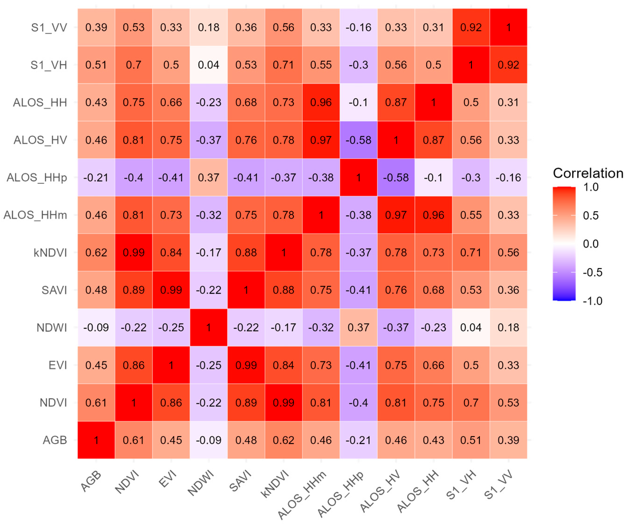
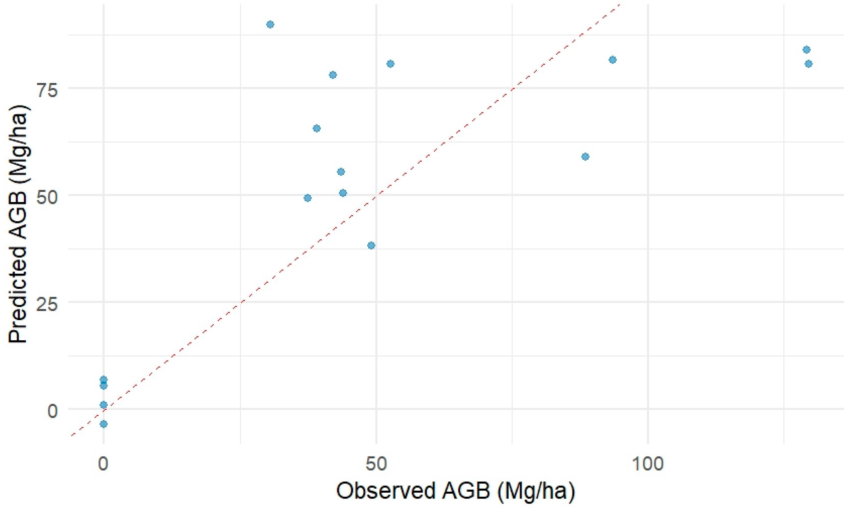
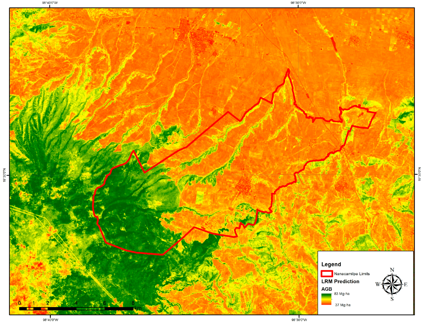
3.3.1. Linear Regression Results

Following the stepwise procedure, the most straightforward linear regression equation was selected based on the Akaike Information Criterion (AIC = 571.67) and the significance of the predictors. The method used selected the simplest linear equation, with the kNDVI as a predictor (Table 3), yielding an acceptable adjustment (R2cv = 0.41; RMSEcv = 25.76) between the observed and predicted values, as determined by the validation process (Figure 5).
Later, we applied the linear model to the data to create a spatial estimation of the aboveground biomass in the study area (Figure 6).

3.3.2. Machine Learning Algorithms

The Random Forest algorithm estimated variable importance by a permutation procedure, which measures the drop in mean accuracy for each variable when this variable is permutated. Meanwhile, XGBoost performs a second-order Taylor expansion for the objective function and uses the second derivative to accelerate the convergence speed of the model while training. The implementation of the models revealed that the variables making significant contributions were those related to the Landsat OLI sensor (NDVI and kNDVI) and the ALOS-Palsar HV polarisation in both cases (Figure 7).
Again, we used the resultant models to predict the spatial distribution of aboveground biomass in the study area. It is worth noting that although both models appear to be visually correct, given that the forest areas are well delineated, the range of biomass differs, especially in areas with no apparent vegetation (Random Forests = 26 to 85 Mg·ha-1 and XGBoost = 9 to 94 Mg·ha−1) (Figure 8).
Although the performance of both models was acceptable according to the metrics used, the Random Forest had a superior performance compared to the XGBoost algorithm (Table 4). However, both models have a relatively small RMSE compared to similar studies [16].
To produce a more explicit spatial distribution map of our models, we ensemble the Random Forests and XGBoost algorithms into one model, allowing us to represent the aboveground biomass with greater detail for the study area (Figure 9).
Finally, we calculated the uncertainty (in the form of standard deviation) for each pixel to identify areas where the models exhibited poor performance. The areas with the highest values of uncertainty were located where the vegetation is denser, such as where the aboveground biomass values were higher (Figure 10).

3.4. Performance Assessment with Independent Data

The comparisons of all estimations against the independent 1 ha forest inventory showed that the XGBoost algorithm performed best, yielding the lowest RMSE and MAE values (73.05 and 58.88 Mg ha−1, respectively) and the second-highest Spearman correlation value (0.64). Our results highlighted that the machine learning algorithms demonstrated superior performance compared to the simple regression model (Table 5); however, all models struggled with higher biomass estimates. It is worth noting that the higher biomass values were registered in pure stands of fir forests (plots 1, 3, 11, and 12). Table 5 reflects this situation, and it is evident that the models used are limited by the capabilities of the sensor used as predictors, as they produced values that are below the actual measurements in the one-hectare plots.

4. Discussion

According to the specialised literature, traditional methods of AGB estimation, such as field-based surveys and inventories, provide reliable data but are limited by spatial coverage and labour intensity [51,52]. The increasing availability of satellite-based remote sensing has introduced a more scalable and efficient approach to AGB estimation, particularly for temperate forests [36,53]. This study uses remote sensing products, freely available to the public, to estimate AGB in forests in central Mexico through two machine learning algorithms and one linear regression approach. In general, the models demonstrated acceptable accuracy levels across different conditions of the study area. For instance, at lower biomass levels (below 90 Mg ha−1), both Random Forest and XGBoost performed adequately, while at higher biomass levels (above 90 Mg ha−1), underestimation became more pronounced. We assume this underestimation is partly due to the saturation effect in the remote sensing signals, where the sensitivity of SAR and optical data diminishes at higher biomass densities [54,55].
Our results demonstrate that combining remote sensing data with machine learning techniques, such as Random Forest and XGBoost, can significantly enhance the accuracy of aboveground biomass (AGB) estimation. They outperform traditional methods by capturing multi-scale image features and integrating various sensor data types, including radar and optical imagery [56]. The models in this study demonstrate superior performance compared to previous work using machine learning algorithms in temperate forest ecosystems in Mexico [57,58]. It is noteworthy that the RMSE in both models is around 20 Mg ha−1, which represents the maximum allowable limit when employing remotely sensed data to estimate aboveground biomass for carbon accounting purposes [59].
It is also important to highlight that the kernel NDVI alone fits the best model in the regression procedure and produces very valuable results. Kernel-based methods have emerged as a powerful tool for non-linear regression and classification, offering the potential to improve the accuracy of biomass estimation by capturing complex relationships between spectral data and biomass [60]. The Kernel NDVI, a modification of the traditional NDVI, incorporates kernel functions to enhance its sensitivity to variations in vegetation structure and biomass. Kernel methods provide a versatile approach to pattern analysis, extending the applicability of linear algorithms to nonlinear problems via the implicit mapping of data into high-dimensional feature spaces. Kernel-based techniques are suitable for handling non-linear relationships between remote sensing data and forest biomass, offering an improved approach to biomass estimation. Kernel NDVI may improve the accuracy of biomass estimation by better representing the complex interactions between vegetation and spectral reflectance [61]. Previous studies have shown that incorporating kernel methods into vegetation indices can improve their performance in estimating vegetation parameters such as leaf area index and biomass [62].
However, problems of overestimation and underestimation remain for all models and predictors. Notably, at higher biomass levels, models underestimated AGB (Table 5) compared to the 1 ha inventory plots. This underestimation is likely due to the saturation effect in synthetic aperture radar (SAR), commonly reported saturation points for L-band SAR (~100 Mg ha−1) [31] and optical data, where signal sensitivity decreases with increasing biomass density. Additionally, the averaging process employed in RF is known to produce results that are biased towards the sample mean. Consequently, estimating both low and high values of aboveground biomass is typically subject to underestimation or overestimation [63]. Nevertheless, it has been demonstrated that XGBoost models of aboveground biomass are more effective than linear regression and RF models in estimating AGB values, irrespective of whether the AGB values are high or low [47].
Our study also highlights the significant contributions found in layers related to the L-band from ALOS PALSAR data (Figure 6). Hensley et al. [64] suggested that L-band backscatter may be more susceptible to aboveground biomass and soil moisture due to surface–volume interactions in less dense forests, such as coniferous forests. This is because it has a high penetration capability through the canopy surface layer and is dispersed by the main trunk and branches of the canopy. Also, the L-band can capture broader scale variation in the horizontal structure of vegetation related to the presence of forest patches with different successional ages and, hence, forest structure [65]. It is also essential to consider the influence of environmental, topographic, and biotic factors on the diverse growing conditions observed in forest areas. These factors affect the distribution of forest biomass and, consequently, the accuracy of biomass estimations [66].
Future research could mitigate this limitation by employing higher-resolution datasets, exploring alternative machine learning algorithms, or utilising hybrid modelling techniques incorporating multiple data sources and methods, as reported by Luo et al. [15]. They employed a hybrid model integrated with four machine learning algorithms (Catboost, XGB, RF, and LightGBM), utilising the entropy weighting method. This model yielded the most accurate predictions compared to the four individual machine learning models for biomass estimations in forest regions of China. Such approaches may help overcome saturation and improve predictions in densely vegetated areas.
Integrating remote sensing data and machine learning provides a robust framework for large-scale biomass estimation, offering significant advantages in terms of spatial coverage, cost-effectiveness, and monitoring capability, as demonstrated in this study. Accurate AGB mapping can support sustainable forest management by identifying areas with high carbon storage potential and tracking changes resulting from natural disturbances or human activities. In addition, more accurate aboveground biomass predictions generated by machine learning algorithms can serve as a basis for predicting aboveground biomass under different future climate scenarios [67]. However, the impact of climate change on aboveground biomass is a relatively long-term process, and long-term field measurement is necessary to predict precise future changes in AGB under changing climate regimes [68].
This information is critical for carbon accounting and climate change mitigation efforts, enabling more effective implementation of forest-based carbon offset programs. Managed temperate forests, such as those in the study area, play a crucial role in climate adaptation strategies. By enhancing carbon sequestration through targeted management practices, these ecosystems contribute to global efforts to mitigate the impacts of climate change. However, there remains a lack of studies assessing the combined effect of future climate change and forest management on biomass and carbon in this region. Furthermore, sustainable forest management supports carbon storage, providing additional ecosystem services, such as water regulation, soil conservation, and biodiversity preservation, which are vital for building resilience against climate impacts.
The findings from this study underscore the potential of multi-sensor approaches and machine learning algorithms for improving biomass estimation accuracy. As remote sensing technologies and modelling techniques continue to advance, further research should focus on refining these methods and exploring the integration of emerging data sources, such as drone-based imagery and advanced hyperspectral sensors. To obtain an accurate estimation of AGB, the fusion of multi-source remotely sensed data and the utilisation of various platforms are necessary.
Additionally, accounting for forest age, species composition, and phenological stages can improve model precision and transferability across forest types. Ultimately, this study supports the idea that the combined use of remote sensing and machine learning represents a promising avenue for improving AGB estimation and informing forest management strategies, thereby contributing to global climate change mitigation and ecosystem conservation efforts.

5. Conclusions

The models used in this study demonstrated varying accuracy across different biomass ranges, with better performance at lower biomass levels and underestimation at higher levels, due to remote sensing signal saturation. The machine learning algorithm Random Forest outperformed (R2cv = 0.54; RMSEcv = 19.17) the regression method (R2cv = 0.41; RMSEcv = 25.76), according to the metrics used. An independent accuracy assessment, utilising additional field data, revealed that machine learning techniques were superior (r = 0.68) to traditional methods (r = 0.50), according to Spearman correlation coefficients. However, all models struggled with higher biomass estimates. Ultimately, we conclude that our findings highlight the potential of integrating machine learning techniques with remote sensing data to improve the reliability of AGB estimation in temperate forests.

Author Contributions

Conceptualisation, M.E.R.-S., A.G.-H. and E.V.-B.; methodology, M.E.R.-S., A.G.-H., E.V.-B., R.P.-M., A.C.-D. and A.D.O.-R.; formal analysis, M.E.R.-S., E.V.-B. and R.P.-M.; investigation A.C.-D. and A.D.O.-R.; writing—original draft preparation, M.E.R.-S., E.V.-B. and A.C.-D.; writing—review and editing, E.V.-B., R.P.-M., A.C.-D. and A.D.O.-R. All authors have read and agreed to the published version of the manuscript.

Funding

This research was funded by the National Institute of Forestry, Agriculture and Livestock Research of Mexico, through the project Explicit spatial estimation of forest aboveground biomass under different remote sensing approaches in the Sierra Nevada, Tlaxcala, Mexico; grant number 12251135086.

Institutional Review Board Statement

Not applicable.

Informed Consent Statement

Not applicable.

Data Availability Statement

Part of the datasets presented in this article are not readily available because the data are part of an ongoing study. Requests to access the datasets should be directed to the corresponding author. The Satellite Imagery used here is available on the Google Earth Engine Platform.

Acknowledgments

The authors acknowledge Nicolas Abad-Zabaleta and Gil Espinoza-Lopez for their technical assistance during the field campaign, and the “Ejido San Jose Nanacamilpa”, Nanacamilpa, Tlaxcala, Mexico, for their support during the development of this research. The authors are deeply grateful for comments and suggestions during the review process, which helped improve the manuscript.

Conflicts of Interest

The authors declare no conflicts of interest. The funders had no role in the study’s design; in the collection, analyses, or interpretation of data; in the writing of the manuscript; or in the decision to publish the results.

References

  1. Reich, P.B.; Bolstad, P. Productivity of Evergreen and Deciduous Temperate Forests. In Terrestrial Global Productivity; Elsevier: Amsterdam, The Netherlands, 2001; pp. 245–283. [Google Scholar]
  2. Ávila-Akerberg, V.; Rosaliano-Evaristo, R.; González-Martínez, T.; Pichardo-García, B.; Serrano-González, D. Classification and Nomenclature of Temperate Forest Types in Mexico. Veg. Classif. Surv. 2023, 4, 329–341. [Google Scholar] [CrossRef]
  3. Canadell, J.G.; Schulze, E.D. Global Potential of Biospheric Carbon Management for Climate Mitigation. Nat. Commun. 2014, 5, 5282. [Google Scholar] [CrossRef] [PubMed]
  4. Law, B.E.; Hudiburg, T.W.; Berner, L.T.; Kent, J.J.; Buotte, P.C.; Harmon, M.E. Land Use Strategies to Mitigate Climate Change in Carbon Dense Temperate Forests. Proc. Natl. Acad. Sci. USA 2018, 115, 3663–3668. [Google Scholar] [CrossRef] [PubMed]
  5. Case, M.J.; Johnson, B.G.; Bartowitz, K.J.; Hudiburg, T.W. Forests of the Future: Climate Change Impacts and Implications for Carbon Storage in the Pacific Northwest, USA. For. Ecol. Manag. 2021, 482, 118886. [Google Scholar] [CrossRef]
  6. Kumar, L.; Sinha, P.; Taylor, S.; Alqurashi, A.F. Review of the Use of Remote Sensing for Biomass Estimation to Support Renewable Energy Generation. J. Appl. Remote Sens. 2015, 9, 097696. [Google Scholar] [CrossRef]
  7. Gómez, C.; White, J.C.; Wulder, M.A. Optical Remotely Sensed Time Series Data for Land Cover Classification: A Review. ISPRS J. Photogramm. Remote Sens. 2016, 116, 55–72. [Google Scholar] [CrossRef]
  8. Aziz, G.; Minallah, N.; Saeed, A.; Frnda, J.; Khan, W. Remote Sensing Based Forest Cover Classification Using Machine Learning. Sci. Rep. 2024, 14, 69. [Google Scholar] [CrossRef]
  9. Ortiz-Reyes, A.D.; Barrera-Ortega, D.; Velasco-Bautista, E.; Romero-Sánchez, M.E.; Correa-Díaz, A. Predicting Forest Parameters through Generalized Linear Mixed Models Using GEDI Metrics in a Temperate Forest in Oaxaca, Mexico. Int. J. Remote Sens. 2024, 45, 8037–8060. [Google Scholar] [CrossRef]
  10. Xu, D.; Wang, H.; Xu, W.; Luan, Z.; Xu, X. LiDAR Applications to Estimate Forest Biomass at Individual Tree Scale: Opportunities, Challenges and Future Perspectives. Forests 2021, 12, 550. [Google Scholar] [CrossRef]
  11. Coops, N.C. Characterizing Forest Growth and Productivity Using Remotely Sensed Data. Curr. For. Rep. 2015, 1, 195–205. [Google Scholar] [CrossRef]
  12. GOFC-GOLD. A Sourcebook of Methods and Procedures for Monitoring and Reporting Anthropogenic Greenhouse Gas Emissions and Removals Associated with Deforestation, Gains and Losses of Carbon Stocks in Forests Remaining Forests, and Forestation; Land Cover Project Office, Wageningen University: Wageningen, The Netherlands, 2015. [Google Scholar]
  13. Chen, L.; Ren, C.; Zhang, B.; Wang, Z.; Xi, Y. Estimation of Forest Above-Ground Biomass by Geographically Weighted Regression and Machine Learning with Sentinel Imagery. Forests 2018, 9, 582. [Google Scholar] [CrossRef]
  14. Issa, S.; Dahy, B.; Ksiksi, T.; Saleous, N. Non-Conventional Methods as a New Alternative for the Estimation of Terrestrial Biomass and Carbon Sequestered. World J. Agric. Soil Sci. 2019, 4, 1–8. [Google Scholar] [CrossRef]
  15. Luo, M.; Anees, S.A.; Huang, Q.; Qin, X.; Qin, Z.; Fan, J.; Han, G.; Zhang, L.; Shafri, H.Z.M. Improving Forest Above-Ground Biomass Estimation by Integrating Individual Machine Learning Models. Forests 2024, 15, 975. [Google Scholar] [CrossRef]
  16. Zhang, Y.; Ma, J.; Liang, S.; Li, X.; Li, M. An Evaluation of Eight Machine Learning Regression Algorithms for Forest Aboveground Biomass Estimation from Multiple Satellite Data Products. Remote Sens. 2020, 12, 4015. [Google Scholar] [CrossRef]
  17. Fan, D.; Biswas, A.; Ahrens, J.P. Explainable AI Integrated Feature Engineering for Wildfire Prediction. arXiv 2024, arXiv:2404.01487. [Google Scholar]
  18. Dittmann, S.; Thiessen, E.; Hartung, E. Applicability of Different Non-Invasive Methods for Tree Mass Estimation: A Review. For. Ecol. Manag. 2017, 398, 208–215. [Google Scholar] [CrossRef]
  19. Jensen, D.; Cavanaugh, K.C.; Simard, M.; Okin, G.S.; Castañeda-Moya, E.; McCall, A.; Twilley, R.R. Integrating Imaging Spectrometer and Synthetic Aperture Radar Data for Estimating Wetland Vegetation Aboveground Biomass in Coastal Louisiana. Remote Sens. 2019, 11, 2533. [Google Scholar] [CrossRef]
  20. Popescu, S.C. Estimating Biomass of Individual Pine Trees Using Airborne Lidar. Biomass Bioenergy 2007, 31, 646–655. [Google Scholar] [CrossRef]
  21. CONAFOR. National System of Forest Information: National Forest and Soils Inventory; CONAFOR: Zapopan, Mexico, 2012. [Google Scholar]
  22. Heris, M.P.; Bagstad, K.J.; Troy, A.R.; O’neil-Dunne, J.P.M. Assessing the Accuracy and Potential for Improvement of the National Land Cover Database’s Tree Canopy Cover Dataset in Urban Areas of the Conterminous United States. Remote Sens. 2022, 14, 1219. [Google Scholar] [CrossRef]
  23. Avendaño Hernandez, D.M.; Acosta Mireles, M.; Carrillo Anzures, F.; Etchevers Barra, J.D. Estimación de Biomasa y Carbono En Un Bosque de Abies Religiosa. Rev. Fitotec. Mex. 2009, 32, 233–238. [Google Scholar] [CrossRef]
  24. Carrillo Anzúres, F.; Acosta Mireles, M.; Flores Ayala, E.; Juárez Bravo, J.E.; Bonilla Padilla, E. Estimación de Biomasa y Carbono en dos Especies Arboreas en la Sierra Nevada, México. Rev. Mex. Cienc. Agric. 2018, 5, 779–793. [Google Scholar] [CrossRef]
  25. Ruiz-Aquino, F.; Valdez-Hernández, J.I.; Manzano-Méndez, F.; Rodríguez-Ortiz, G.; Romero-Manzanares, A.; Fuentes-López, M.E. Ecuaciones de Biomasa Aérea Para Quercus Laurina y Q. Crassifolia En Oaxaca. Madera Bosques 2014, 20, 33–48. [Google Scholar] [CrossRef]
  26. Aguilar-Hernández, L.; García-Martínez, R.; Gómez-Miraflor, A.; Martínez-Gómez, O. Estimación de Biomasa Mediante La Generación de Una Ecuación Alométrica Para Madroño (Arbutus xalapensis). In Proceedings of the IV Congreso Internacional y XVIII Congreso Nacional de Ciencias Agronómicas, Texcoco, Mexico, 20–22 April 2016; pp. 529–530. (In Spanish). [Google Scholar]
  27. Šmelko, Š.; Merganič, J. Some Methodological Aspects of the National Forest Inventory and Monitoring in Slovakia. J. For. Sci. 2008, 54, 476–483. [Google Scholar] [CrossRef]
  28. Ao, W.; Xu, F. Robust Ship Detection in SAR Images from Complex Background. In Proceedings of the 2018 IEEE International Conference on Computational Electromagnetics (ICCEM), Chengdu, China, 26–28 March 2018; IEEE: Piscataway, NJ, USA, 2018; pp. 1–2. [Google Scholar]
  29. Shimada, M.; Itoh, T.; Motooka, T.; Watanabe, M.; Shiraishi, T.; Thapa, R.; Lucas, R. New Global Forest/Non-Forest Maps from ALOS PALSAR Data (2007–2010). Remote Sens. Environ. 2014, 155, 13–31. [Google Scholar] [CrossRef]
  30. Duong-Nguyen, T.-B.; Hoang, T.-N.; Vo, P.; Le, H.-B. Water Level Estimation Using Sentinel-1 Synthetic Aperture Radar Imagery and Digital Elevation Models. arXiv 2020, arXiv:2012.07627. [Google Scholar]
  31. Hernández-Stefanoni, J.L.; Castillo-Santiago, M.Á.; Mas, J.F.; Wheeler, C.E.; Andres-Mauricio, J.; Tun-Dzul, F.; George-Chacón, S.P.; Reyes-Palomeque, G.; Castellanos-Basto, B.; Vaca, R.; et al. Improving Aboveground Biomass Maps of Tropical Dry Forests by Integrating LiDAR, ALOS PALSAR, Climate and Field Data. Carbon Balance Manag. 2020, 15, 15. [Google Scholar] [CrossRef]
  32. Imangholiloo, M.; Rasinmäki, J.; Rauste, Y.; Holopainen, M. Utilizing Sentinel-1A Radar Images for Large-Area Land Cover Mapping with Machine-Learning Methods. Can. J. Remote Sens. 2019, 45, 163–175. [Google Scholar] [CrossRef]
  33. Radočaj, D.; Obhođaš, J.; Jurišić, M.; Gašparović, M. Global Open Data Remote Sensing Satellite Missions for Land Monitoring and Conservation: A Review. Land 2020, 9, 402. [Google Scholar] [CrossRef]
  34. Kakoullis, D.; Fotiou, K.; Ibarrola Subiza, N.; Brcic, R.; Eineder, M.; Danezis, C. An Advanced Quality Assessment and Monitoring of ESA Sentinel-1 SAR Products via the CyCLOPS Infrastructure in the Southeastern Mediterranean Region. Remote Sens. 2024, 16, 1696. [Google Scholar] [CrossRef]
  35. Yan, L.; Roy, D.; Zhang, H.; Li, J.; Huang, H. An Automated Approach for Sub-Pixel Registration of Landsat-8 Operational Land Imager (OLI) and Sentinel-2 Multi Spectral Instrument (MSI) Imagery. Remote Sens. 2016, 8, 520. [Google Scholar] [CrossRef]
  36. Zhu, X.; Liu, D. Improving Forest Aboveground Biomass Estimation Using Seasonal Landsat NDVI Time-Series. ISPRS J. Photogramm. Remote Sens. 2015, 102, 222–231. [Google Scholar] [CrossRef]
  37. Huete, A.R. A Soil-Adjusted Vegetation Index (SAVI). Remote Sens. Environ. 1988, 25, 295–309. [Google Scholar] [CrossRef]
  38. Waring, R.H.; Coops, N.C.; Fan, W.; Nightingale, J.M. MODIS Enhanced Vegetation Index Predicts Tree Species Richness across Forested Ecoregions in the Contiguous U.S.A. Remote Sens. Environ. 2006, 103, 218–226. [Google Scholar] [CrossRef]
  39. Gao, B. NDWI—A Normalized Difference Water Index for Remote Sensing of Vegetation Liquid Water from Space. Remote Sens. Environ. 1996, 58, 257–266. [Google Scholar] [CrossRef]
  40. Camps-Valls, G.; Campos-Taberner, M.; Moreno-Martínez, Á.; Walther, S.; Duveiller, G.; Cescatti, A.; Mahecha, M.D.; Muñoz-Marí, J.; García-Haro, F.J.; Guanter, L.; et al. A Unified Vegetation Index for Quantifying the Terrestrial Biosphere. Sci. Adv. 2021, 7, eabc7447. [Google Scholar] [CrossRef]
  41. Wang, Q.; Moreno-Martínez, Á.; Muñoz-Marí, J.; Campos-Taberner, M.; Camps-Valls, G. Estimation of Vegetation Traits with Kernel NDVI. ISPRS J. Photogramm. Remote Sens. 2023, 195, 408–417. [Google Scholar] [CrossRef]
  42. R Core Team. R: A Language and Environment for Statistical Computing, version 4.1.0; R Foundation for Statistical Computing: Vienna, Austria, 2020. [Google Scholar]
  43. Romero-Sanchez, M.E.; Ponce-Hernandez, R. Assessing and Monitoring Forest Degradation in a Deciduous Tropical Forest in Mexico via Remote Sensing Indicators. Forests 2017, 8, 302. [Google Scholar] [CrossRef]
  44. Breiman, L. Random Forests. Mach. Learn. 2001, 45, 5–32. [Google Scholar] [CrossRef]
  45. Luan, J.; Zhang, C.; Xu, B.; Xue, Y.; Ren, Y. The Predictive Performances of Random Forest Models with Limited Sample Size and Different Species Traits. Fish Res. 2020, 227, 105534. [Google Scholar] [CrossRef]
  46. Chen, T.; Guestrin, C. Xgboost: A Scalable Tree Boosting System. In Proceedings of the 22nd ACM SIGKDD International Conference on Knowledge Discovery and Data Mining, San Francisco, CA, USA, 13–17 August 2016; pp. 785–794. [Google Scholar]
  47. Li, Y.; Li, M.; Li, C.; Liu, Z. Forest Aboveground Biomass Estimation Using Landsat 8 and Sentinel-1A Data with Machine Learning Algorithms. Sci. Rep. 2020, 10, 9952. [Google Scholar] [CrossRef]
  48. Rossiter, D.G. Spatial Analysis with the R Project for Statistical Computing; Cornell University: Wageningen, The Netherlands, 2008. [Google Scholar]
  49. Carlón Allende, T.; Mendoza, M.E.; Pérez-Salicrup, D.R.; Villanueva-Díaz, J.; Lara, A. Climatic Responses of Pinus Pseudostrobus and Abies Religiosa in the Monarch Butterfly Biosphere Reserve, Central Mexico. Dendrochronologia 2016, 38, 103–116. [Google Scholar] [CrossRef]
  50. Torres-Rojas, G.; Romero-Sánchez, M.E.; Velasco-Bautista, E.; González-Hernández, A. Estimación de Parámetros Forestales En Bosques de Coníferas Con Técnicas de Percepción Remota. Rev. Mex. Cienc. For. 2016, 7, 7–24. [Google Scholar]
  51. Moreno-Fernández, D.; Cañellas, I.; Hernández, L.; Adame, P.; Alberdi, I. Nested Plot Designs Used in Forest Inventory Do Not Accurately Capture Tree Species Richness in Southwestern European Forests. Ann. For. Sci. 2024, 81, 20. [Google Scholar] [CrossRef]
  52. Shendryk, Y. Fusing GEDI with Earth Observation Data for Large Area Aboveground Biomass Mapping. Int. J. Appl. Earth Obs. Geoinf. 2022, 115, 103108. [Google Scholar] [CrossRef]
  53. Wulder, M.A.; Hermosilla, T.; White, J.C.; Coops, N.C. Biomass Status and Dynamics over Canada’s Forests: Disentangling Disturbed Area from Associated Aboveground Biomass Consequences. Environ. Res. Lett. 2020, 15, 094093. [Google Scholar] [CrossRef]
  54. Häme, T.; Rauste, Y.; Antropov, O.; Ahola, H.A.; Kilpi, J. Improved Mapping of Tropical Forests with Optical and Sar Imagery, Part Ii: Above Ground Biomass Estimation. IEEE J. Sel. Top. Appl. Earth Obs. Remote Sens. 2013, 6, 92–101. [Google Scholar] [CrossRef]
  55. Urbazaev, M.; Thiel, C.; Cremer, F.; Dubayah, R.; Migliavacca, M.; Reichstein, M.; Schmullius, C. Estimation of Forest Aboveground Biomass and Uncertainties by Integration of Field Measurements, Airborne LiDAR, and SAR and Optical Satellite Data in Mexico. Carbon Balance Manag. 2018, 13, 5. [Google Scholar] [CrossRef]
  56. Schwartz, M.; Ciais, P.; Ottlé, C.; De Truchis, A.; Vega, C.; Fayad, I.; Brandt, M.; Fensholt, R.; Baghdadi, N.; Morneau, F.; et al. High-Resolution Canopy Height Map in the Landes Forest (France) Based on GEDI, Sentinel-1, and Sentinel-2 Data with a Deep Learning Approach. Int. J. Appl. Earth Obs. Geoinf. 2024, 128, 103711. [Google Scholar] [CrossRef]
  57. Cartus, O.; Kellndorfer, J.; Walker, W.; Franco, C.; Bishop, J.; Santos, L.; Fuentes, J. A National, Detailed Map of Forest Aboveground Carbon Stocks in Mexico. Remote Sens. 2014, 6, 5559–5588. [Google Scholar] [CrossRef]
  58. Rosas-Chavoya, M.; López-Serrano, P.M.; Vega-Nieva, D.J.; Hernández-Díaz, J.C.; Wehenkel, C.; Corral-Rivas, J.J. Estimating Above-Ground Biomass from Land Surface Temperature and Evapotranspiration Data at the Temperate Forests of Durango, Mexico. Forests 2023, 14, 299. [Google Scholar] [CrossRef]
  59. Zolkos, S.G.; Goetz, S.J.; Dubayah, R. A Meta-Analysis of Terrestrial Aboveground Biomass Estimation Using Lidar Remote Sensing. Remote Sens. Environ. 2013, 128, 289–298. [Google Scholar] [CrossRef]
  60. Jin, Y.; Yang, X.; Qiu, J.; Li, J.; Gao, T.; Wu, Q.; Zhao, F.; Ma, H.; Yu, H.; Xu, B. Remote Sensing-Based Biomass Estimation and Its Spatio-Temporal Variations in Temperate Grassland, Northern China. Remote Sens. 2014, 6, 1496–1513. [Google Scholar] [CrossRef]
  61. Bhandari, A.K.; Kumar, A.; Singh, G.K. Feature Extraction Using Normalized Difference Vegetation Index (NDVI): A Case Study of Jabalpur City. Procedia Technol. 2012, 6, 612–621. [Google Scholar] [CrossRef]
  62. Xu, H.; Yin, H.; Liu, J.; Wang, L.; Feng, W.; Song, H.; Fan, Y.; Qi, K.; Liang, Z.; Li, W.; et al. Prediction of Spatial Winter Wheat Yield by Combining Multiscale Time Series of Vegetation and Meteorological Indices. Agronomy 2025, 15, 1114. [Google Scholar] [CrossRef]
  63. Xu, L.; Saatchi, S.S.; Yang, Y.; Yu, Y.; White, L. Performance of Non-Parametric Algorithms for Spatial Mapping of Tropical Forest Structure. Carbon Balance Manag. 2016, 11, 18. [Google Scholar] [CrossRef]
  64. Hensley, S.; Oveisgharan, S.; Saatchi, S.; Simard, M.; Ahmed, R.; Haddad, Z. An Error Model for Biomass Estimates Derived from Polarimetric Radar Backscatter. IEEE Trans. Geosci. Remote Sens. 2014, 52, 4065–4082. [Google Scholar] [CrossRef]
  65. Huang, H.; Liu, C.; Wang, X.; Zhou, X.; Gong, P. Integration of Multi-Resource Remotely Sensed Data and Allometric Models for Forest Aboveground Biomass Estimation in China. Remote Sens. Environ. 2019, 221, 225–234. [Google Scholar] [CrossRef]
  66. Tian, L.; Wu, X.; Tao, Y.; Li, M.; Qian, C.; Liao, L.; Fu, W. Review of Remote Sensing-Based Methods for Forest Aboveground Biomass Estimation: Progress, Challenges, and Prospects. Forests 2023, 14, 1086. [Google Scholar] [CrossRef]
  67. Li, Y.; Li, M.; Wang, Y. Forest Aboveground Biomass Estimation and Response to Climate Change Based on Remote Sensing Data. Sustainability 2022, 14, 14222. [Google Scholar] [CrossRef]
  68. Zhang, Y.; Liang, S.; Yang, L. A Review of Regional and Global Gridded Forest Biomass Datasets. Remote Sens. 2019, 11, 2744. [Google Scholar] [CrossRef]
Figure 1. Localisation of the study area.
Geomatics 05 00030 g001
Figure 2. Forest inventory in Nanacamilpa, Tlaxcala. A green square equals 1 ha.
Geomatics 05 00030 g002
Figure 3. Distribution of aboveground biomass among 1 ha plots.
Geomatics 05 00030 g003
Figure 4. Correlation Heatmap of AGB and predictors.
Geomatics 05 00030 g004
Figure 5. Predicted vs. observed aboveground biomass.
Geomatics 05 00030 g005
Figure 6. Aboveground biomass estimation with a linear regression model.
Geomatics 05 00030 g006
Figure 7. Variable importance across models.
Geomatics 05 00030 g007
Figure 8. Aboveground biomass predictions: Random Forest (left) and XGBoost (right).
Geomatics 05 00030 g008
Figure 9. Aboveground biomass prediction with the ensemble models.
Geomatics 05 00030 g009
Figure 10. Uncertainty associated with the model predictions.
Geomatics 05 00030 g010
Table 2. Variables derived from remote sensing sensors.
SensorLayer
ALOS PALSARHH, HH+HV, HH-HV, HV
Sentinel 1VH, VV, VV+VH, V-VH
Landsat OLINDVI, EVI, SAVI, NDWI, kNDVI
Table 3. Metrics for linear regression performance.
CoefficientsEstimateStd. Errort-ValuePr (>|t|)
Intercept53.7424.24912.65<0.001
kNDVI23.8114.1485.74<0.001
Table 4. Metrics for model performance.
ModelR2cvRMSEcv (Mg ha−1)
Random Forest0.5419.17
XGBoost0.3926.32
Table 5. Values of aboveground biomass for comparison purposes.
PlotAGB
(Measured)
LMEnsembledRandom ForestXGBoost
Mg ha−1
1198.4777.4275.5672.1878.94
284.4375.5473.5170.2476.77
3154.6480.0576.7573.4780.04
4164.0374.8273.9171.0576.77
5111.6573.6873.6970.6276.76
673.1172.8573.7970.8276.76
7142.3272.6773.7970.8276.76
8105.5873.8873.7870.7976.76
9102.1772.8070.4071.6769.13
11142.1678.8175.7772.6178.94
12219.4077.6875.4371.9378.94
S0.500.680.590.64
RMSE74.1775.5077.9973.05
MAE60.7062.0864.7058.88
Disclaimer/Publisher’s Note: The statements, opinions and data contained in all publications are solely those of the individual author(s) and contributor(s) and not of MDPI and/or the editor(s). MDPI and/or the editor(s) disclaim responsibility for any injury to people or property resulting from any ideas, methods, instructions or products referred to in the content.

