Land Use and Land Cover (LULC) Mapping Accuracy Using Single-Date Sentinel-2 MSI Imagery with Random Forest and Classification and Regression Tree Classifiers

Abstract

The use of Google Earth Engine (GEE), a cloud-based computing platform, in spatio-temporal evaluation studies has increased rapidly in natural sciences such as forestry. In this study, Sentinel-2 satellite imagery and Shuttle Radar Topography Mission (SRTM) elevation data and image classification algorithms based on two machine learning techniques were examined. Random Forest (RF) and Classification and Regression Trees (CART) were used to classify land use and land cover (LULC) in western Oregon (USA). To classify the LULC from the spectral bands of satellite images, a composition consisting of vegetation difference indices NDVI, NDWI, EVI, and BSI, and a digital elevation model (DEM) were used. The study area was selected due to a diversity of land cover types including research forest, botanical gardens, recreation area, and agricultural lands covered with diverse plant species. Five land classes (forest, agriculture, soil, water, and settlement) were delineated for LULC classification testing. Different spatial points (totaling 75, 150, 300, and 2500) were used as training and test data. The most successful model performance was RF, with an accuracy of 98% and a kappa value of 0.97, while the accuracy and kappa values for CART were 95% and 0.94, respectively. The accuracy of the generated LULC maps was evaluated using 500 independent reference points, in addition to the training and testing datasets. Based on this assessment, the RF classifier that included elevation data achieved an overall accuracy of 92% and a kappa coefficient of 0.90. The combination of vegetation difference indices with elevation data was successful in determining the areas where clear-cutting occurred in the forest. Our results present a promising technique for the detection of forests and forest openings, which was helpful in identifying clear-cut sites. In addition, the GEE and RF classifier can help identify and map storm damage, wind damage, insect defoliation, fire, and management activities in forest areas.

1. Introduction

Natural disasters are a frequent occurrence and can sometimes have devastating impacts. However, in recent years, the increasing frequency of natural disasters with significant effects on people has reached new levels. It is observed that natural disasters mostly occur in Asia followed by Africa, America, and Europe. Asian countries were among the most affected by the devastating natural events that occurred between 1995 and 2022 [1]. To prevent natural disasters and raise awareness, scientists have conducted numerous studies that have dealt with important issues such as the political, cultural, social, and economic aspects that concern both management and individuals [2,3]. In these studies, satellite images with varying temporal and spatial resolutions have been used to monitor land changes and forest ecosystems in mountainous regions, helping to mitigate the impact of devastating natural disasters and human disturbances on Earth.

Forests provide many direct and indirect ecosystem services to human beings such as protecting biodiversity, storing carbon, and regulating the water cycle. In engineering-based activities, technological measurement tools and applications have been used to conduct research, observation, and detection studies before and after natural disasters. Studies involving the monitoring of land use and land cover (LULC) changes can be carried out on local or regional scales as well as on global scales [4,5]. Remote sensing (RS) techniques can be very beneficial in detecting and monitoring natural disasters, especially those affecting natural habitats [6]. It is almost impossible to completely prevent catastrophic natural events in dynamic ecosystems. However, in order to reduce the impact of natural disasters, it is necessary to conduct more studies particularly in lakes, coral reefs, oceans, forests, and arid lands [7]. For the purpose of the sustainable planning of large ecosystems such as forests, effective data analysis tools and approaches that can be flexibles over time are rapidly increasing [8]. The use of advanced mathematical calculations and cloud computing platforms with traditional RS- and geographical information systems (GIS)-based techniques is increasing in natural resource research.

Traditional research methods are not time effective or cost efficient in monitoring large ecosystems. Modern tools such as RS technologies and GIS can provide faster and more comprehensive data in larger areas. The algorithms and data libraries developed in recent years have been effectively used in individual or institutional research in spatial data analysis with tools such as GEE. Hence, the popularity of RS- and GIS-based analyses in large study areas such as forestry has increased through the use of GEE-based studies. This increase can be expected to accelerate in the coming years as GEE provides access to cost-effective RS and GIS tools with data at local, regional, and global scales [9,10,11]. Many LULC change analyses have been carried out using RS and geographic data [12]. Most recently, machine learning-based studies have become increasingly popular for land change and cover classification models.

In many countries, especially in the USA, mapping and analyses are increasingly carried out by using the GEE platform for various research topics such as forest mapping, drought monitoring, land use/land cover, fire, surface water detection, paddy rice, flood, snow, mine mapping, disease risk mapping, lake and river mapping, crop yield estimation, evapotranspiration, shoreline, wetland, albedo trend, urban, soil, species habitat monitoring, and natural hazard management [10,13,14,15,16,17,18,19]. Factors such as increased human activities and climate change put pressure on forest–agricultural ecosystems. As a result of this pressure, changes in LULC require more attention for successful land management. Monitoring forest and agricultural areas and detecting land change are vital elements in environmental sustainability and successful planning. In other words, the negative effects of rapid and unplanned construction on different ecosystems can be reduced by creating land suitability models. As a result, planners are guided by creating models that can prevent the human-induced degradation of human environments [20,21].

There are challenges in analyzing multiple data sources (vegetation difference indices and topographic, climatic, social, and economic data) with machine learning techniques. However, high accuracy image classifiers such as RF and CART can overcome these difficulties and are widely used methods for LULC [22,23,24]. In the classification studies of RS data using machine learning techniques, data quality and preferred decision tree size have an effect on classification success [25]. Classification performed with satellite images uses data types obtained with band ratio techniques rather than using a single band. The aim of this is to increase the classification success and reduce noise while performing satellite image classification [4]. In addition, the use of multiple data sources, such as the use of topographic data and time series, which can increase accuracy, affects accuracy, especially in big data classification studies [23,26]. Therefore, LULC studies have investigated using satellite images, the content of the planning and the accuracy of the classification performed, the choice of classifier, and the size of the area.

We created LULC maps for a small city with multiple land cover types on the GEE cloud computing platform. Our objectives were to use a cloud environment to test LULC classification accuracies and the influence of spectral indices, different numbers of test points, and elevation data. Our LULC classification process applied the RF and CART algorithms, which are well-known machine learning techniques. LULC was estimated with the composition of the indices produced by the ratio of the spectral bands of Sentinel-2 and a DEM. The sensitivities and responses of the classifiers to the data composition used, and the training and test data were examined. This study not only explains LULC mapping precision but also presents applicable insights for forest management, including the detection of disturbances such as clear-cutting. These insights can help inform decision makers and researchers in geomatics and environmental monitoring.

2. Materials and Methods

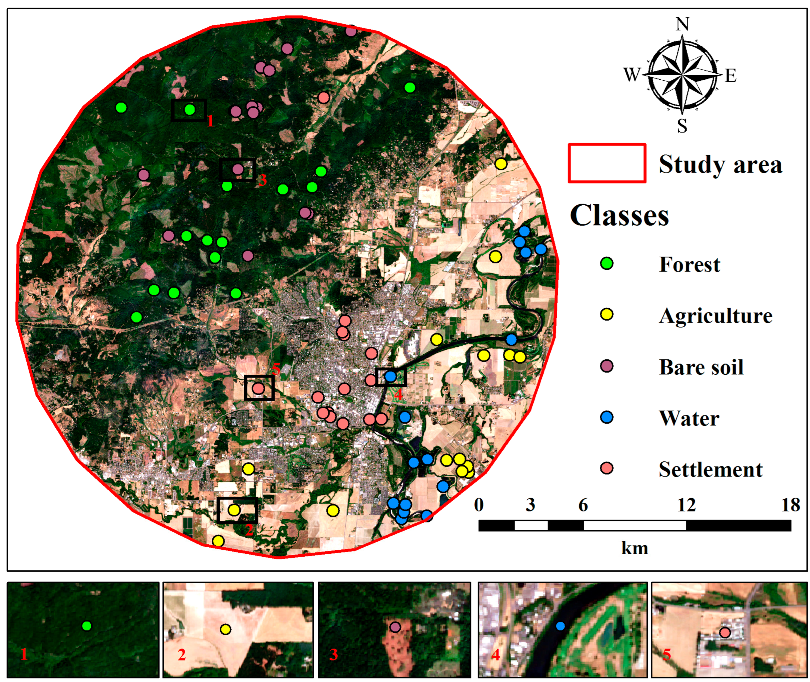
2.1. Study Area

Land use/cover classification involved areas surrounding the city of Corvallis (OR, USA) with the RF and CART machine learning algorithms. The main study area, situated at approximately 44.603° N, −123.301° W, has a temperate oceanic climate with rainy winters and dry summers, which influences vegetation patterns and seasonal land cover dynamics—an important factor for LULC modeling using remote sensing data. The GEE code editor and its provider services were used as a calculation platform. Sentinel-2R satellite images involving the summer season (between 1 April 2023 and 31 July 2023) were analyzed. To compare and check the accuracy of the classifiers, additional training and test subsets were added for each class. In the study, five land classes were evaluated with a range spanning 75 to 2500 ground sampling points created for each class (Figure 1). An accuracy analysis of classifications was also performed for both the RF and CART techniques. Then, differences in the generated land use/cover maps were used to compare the results of CART and RF. For image classification, different training and test datasets were used for different combinations. In this study, land use/cover classes were divided into five groups, which were represented as “1 = forest”, “2 = agriculture”, “3 = bare soil”, “4 = water”, and “5 = settlement”. The settlement category includes urban features such as buildings, roadways, and all infrastructure components in the area.

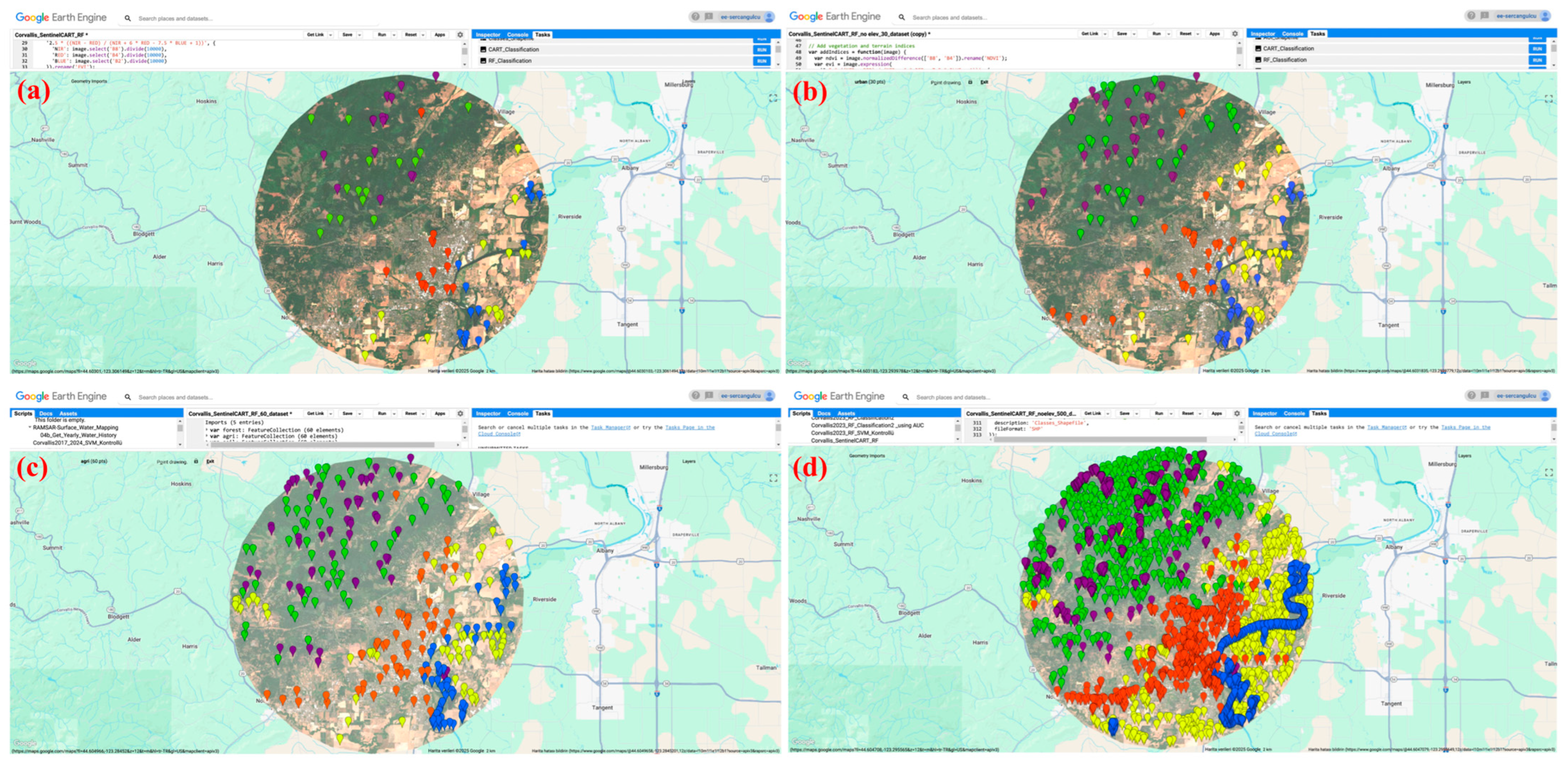
2.2. Data Acquisition and Processing

We used Sentinel-2 (S2) surface reflectance (SR) image satellite bands to generate surface reflectance data from 1 April 2023 to 31 July 2023. A cloud cover filter was applied to include only images with less than 20% cloudy pixels. Clouds and shadows were also masked using the QA60 band [27]. A total of 48 images (“COPERNICUS/S2_SR”) belonging to the specified date range were processed in the GEE environment for the purpose of creating a mosaic [28]. The best 48 images were selected for analysis based on cloud-free conditions. Calculations were made by increasing the accuracy effect of the dataset distribution and amount on the multi-layer (indices and DEM) classification by doubling the existing dataset. Group labels were used for classification methods for ease of use.

The filtered Sentinel-2 images were mosaicked to create a single composite image. The mosaic was cut into a 10 km radius area from the defined center point (lat: 44.603 and lon: −123.301) to focus on the study area (Figure 1). In this study, SRTMGL1_003 data created by the United States Geological Survey (USGS) were used to determine the topographic features of the region [29]. Elevation values on the study area were used for classification purposes. In addition, B2 (blue), B3 (green), B4 (red), B8 (near infrared), and B11 (shortwave infrared) bands of S2 satellite were preferred to calculate the spectral indices from the images (

Table 1. Specification of S2 bands used in this study.

Band Number	Central Wavelength (nm)	Resolution (m)
2	490	10
3	560	10
4	665	10
8	842	10
11	1610	20

). The final database was created by making a median composite of all bands.

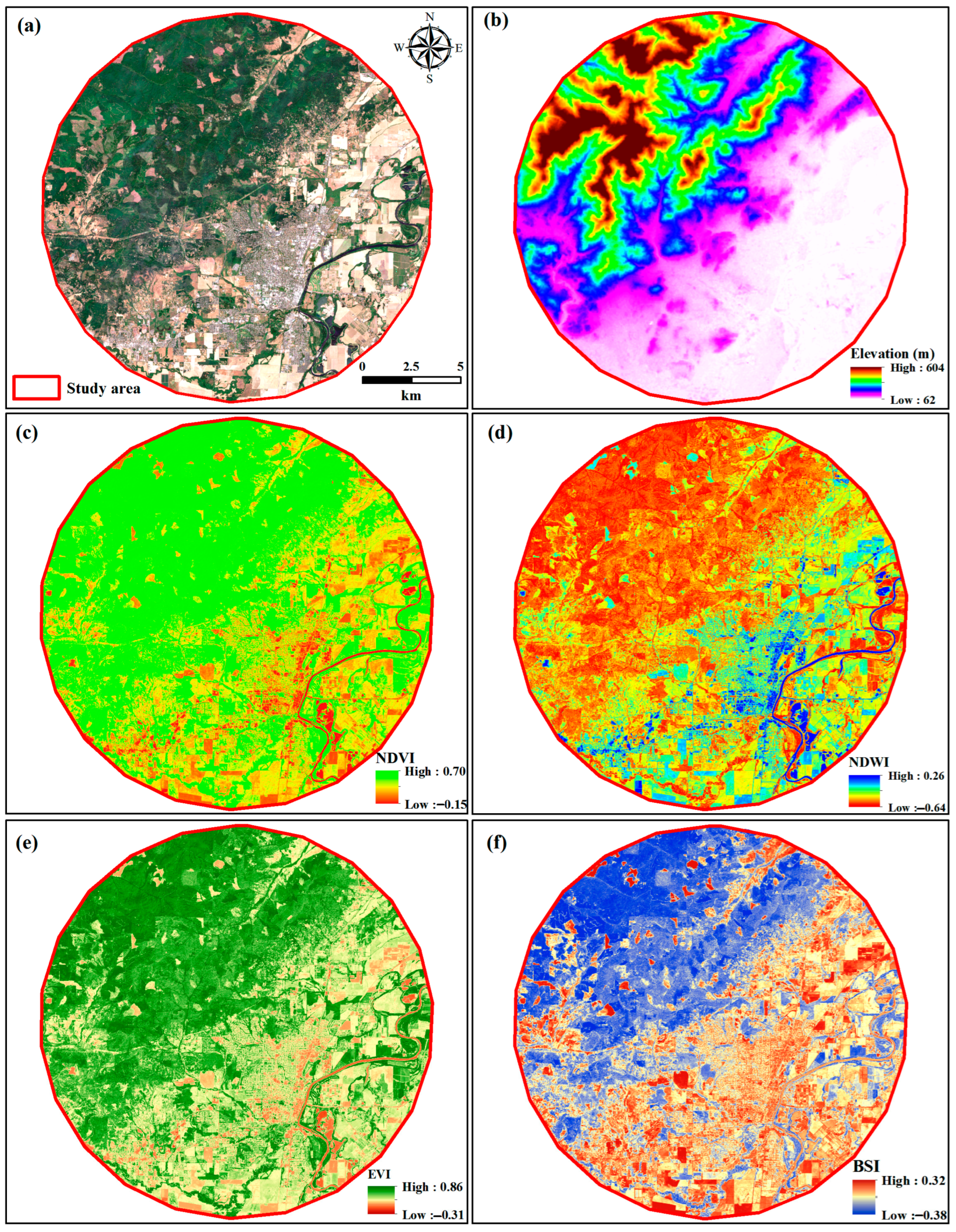
2.3. Vegetation Indices and Terrain Data

Considering mostly preferred bands for land, water, and atmospheric analysis, vegetation indices and terrain were derived on the GEE platform and the resulting values were evaluated in the classification and analysis stages. A global-scale DEM with a resolution of approximately 30 m was provided in GEE as USGS/SRTMGL1_003. The elevation data has an error rate ranging from 16 to 20 m, and was collected by the Shuttle Radar Topography Mission (STRM) [29,30]. In order to increase the success of LULC classification, indices produced by band ratio techniques are widely used. Therefore, various spectral indices were calculated using S2 satellite bands (Figure 2). The java code block used in indices calculations for S2 bands is indicated below. Each index is calculated on the GEE platform with the help of the formulas presented in the code block for the defined band combinations.

var addIndices = function(image) {   var ndvi = image.normalizedDifference(['B8', 'B4']).rename('NDVI');   var evi = image.expression(     '2.5 * ((IR - RED)/(IR + 6 * RED - 7.5 * BLUE + 1))', {       'IR': image.select('B8').divide(10000),       'RED': image.select('B4').divide(10000),       'BLUE': image.select('B2').divide(10000)     }).rename('EVI');   var ndwi = image.normalizedDifference(['B3', 'B8']).rename('NDWI');   var bsi = image.expression(       '((SWIR1 + RED) - (NIR + BLUE))/((SWIR1 + RED) + (NIR + BLUE))', {       'SWIR1': image.select('B11'),       'RED': image.select('B4'),       'NIR': image.select('B8'),       'BLUE': image.select('B2')     }).rename('BSI');   return image.addBands([ndvi, evi, ndwi, bsi]); };

The Normalized Difference Vegetation Index (NDVI) is often used to assess the health and density of vegetation. NDVI represents unitless values between −1 and +1. In areas where there is healthy and dense vegetation, index values approach +1. This index was calculated using the near infrared (B8) and red (B4) bands [31].

The Enhanced Vegetation Index (EVI) was developed to better monitor vegetation, especially in areas with high biomass. The range of values for EVI is unitless and spans −1 to 1, with healthy vegetation generally around 0.20 to 0.80. EVI was calculated using the near infrared (B8), red (B4), and blue (B2) bands [32,33,34].

The Normalized Difference Water Index (NDWI) is represented by unitless values between −1 and +1 and is obtained by dividing the green wavelength (B3) and the near infrared wavelength (B8) by their sum in order to separate the water surfaces from soil and vegetation cover. In areas where there is a lot of vegetation, the index values approach −1. In areas with water bodies, the value increases towards +1 [35].

The Bare Soil Index (BSI) is designed to describe bare soil surfaces using the shortwave infrared (B11), red (B4), near infrared (B8), and blue (B2) bands. In areas where soil mass increases, the unitless value increases towards +1.

2.4. RF and CART Classifiers

RF has a very compatible algorithm for studies such as nonlinear LULC classification [36]. The RF classifier (smileRandomForest function in GEE) was trained using 50 decision trees for all parameters. It can be summarized as a simple decision tree-based classifier and is similar to the classification and regression tree (CART) algorithm, which was first introduced by [37]. The classifier.smileCart command was used on the GEE platform. Both the RF and CART methods are part of the supervised classification category under machine learning techniques [38]. A total of 75, 150, 300, and 2500 spatial points were generated for the training and accuracy dataset from the S2 red–green–blue (RGB) composite (Figure 3). We chose these sample point distributions to represent a wide range of values for comparison and used these distributions for all algorithm comparisons. Training data for five land cover classes—forest, agriculture, water, urban, and bare land—were created. The dataset was randomly split into training (75%) and testing (25%) subsets for classification accuracy assessment. The classified maps and comparison map were exported (with the use of the Export.image.toDrive function of the GEE) to Google Drive as Geotiff images for further analysis.

2.5. Accuracy Assessment

Overall accuracy (OA) is commonly used with parametric data for estimating the accuracy of image classification. Considering the test dataset, OA was calculated as a percentage unit for the correctly classified imagery. Additionally, confusion matrix, user accuracy, producer accuracy, and kappa statistics (measure of agreement) were utilized to further evaluate the class-level performance of RF and CART [39,40,41,42]. To calculate accuracy parameters, 25% of the ground sampling points were randomly used. The classifier.confusionMatrix(), the errorMatrix(), and ConfusionMatrix.kappa() functions in the GEE database were used [25]. Accuracy metrics were exported to Google Drive as *.CSV files for further analysis. In order to compare the LULC maps produced with a small number of test and training data points, the prediction map produced with the test and training dataset was used. In addition to the training and testing datasets, an independent set of 500 control points was used for the accuracy assessment of the produced LULC maps. Using confusion matrix tables, the overall accuracies and kappa coefficients of the resulting thematic maps were calculated.

3. Results

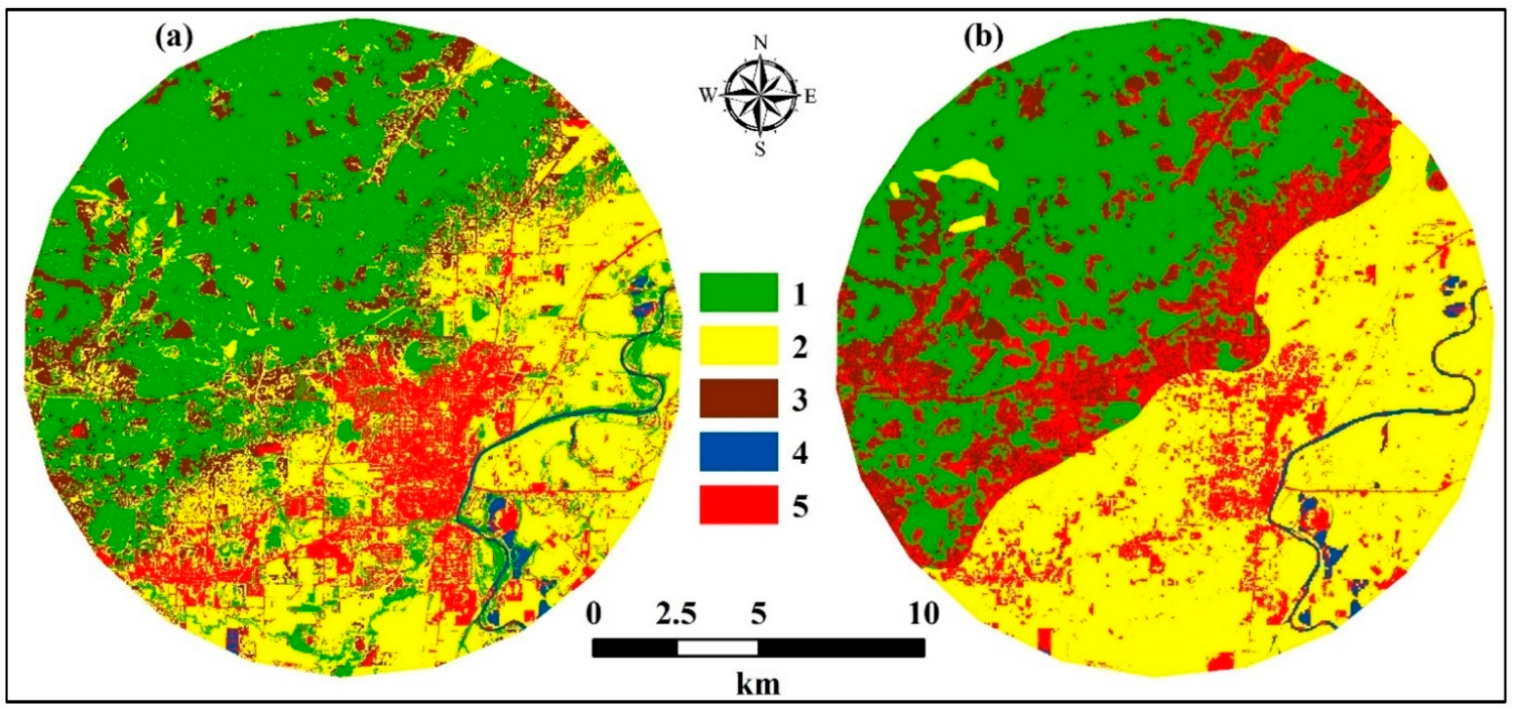
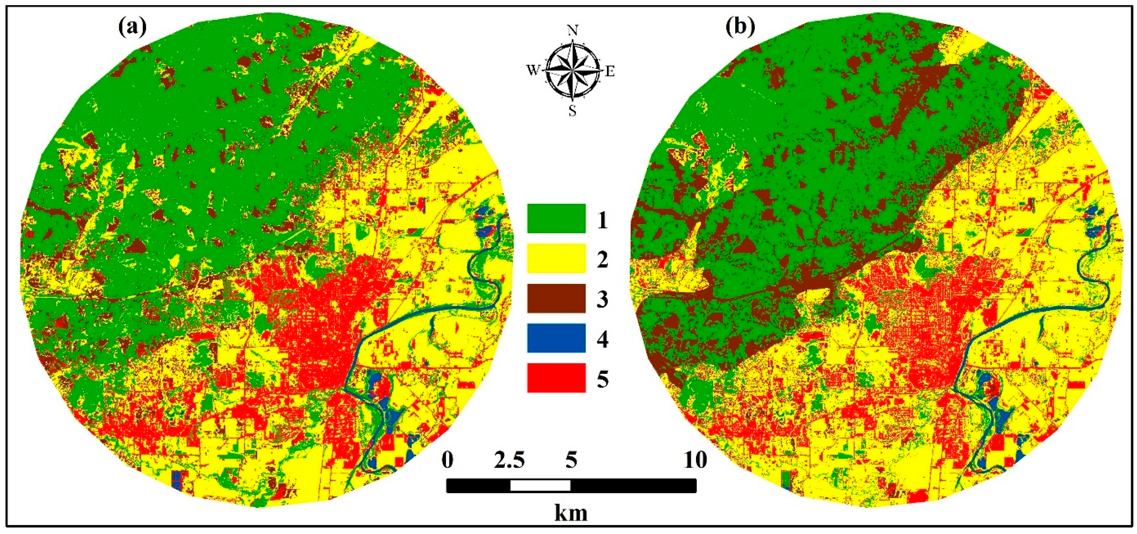
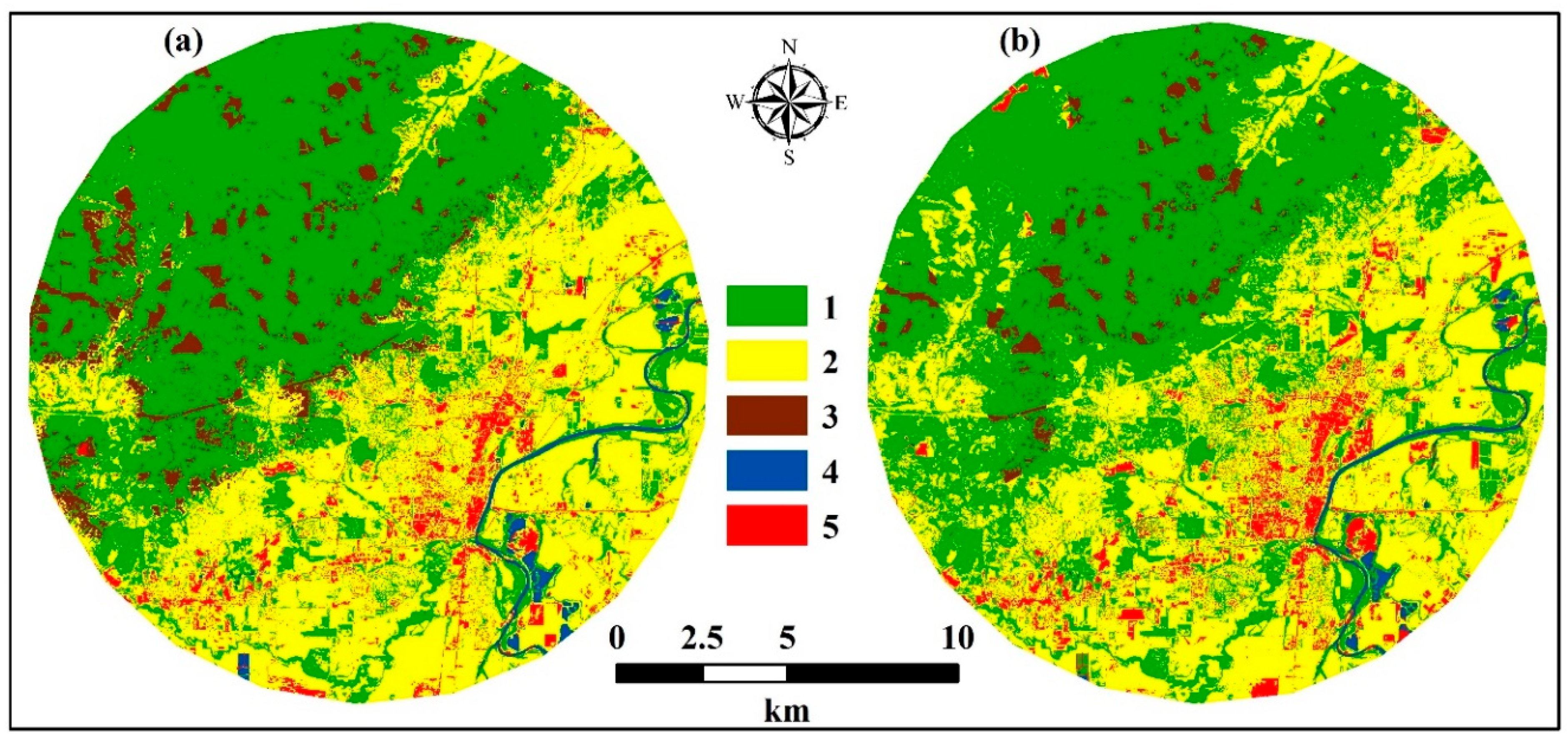
3.1. LULC Classification Maps Without Elevation

The LULC map was divided into five classes with two methods, Random Forest (RF) and CART, with an initial total of 75 training and test points. The composite layers in the classification process included NDVI, NDWI, EVI, and BSI (Figure 4). The RF method estimated 44.63% of the total area as “forest”, while the CART method estimated this rate slightly lower at 43.74%. RF estimated 34.82% of the area as “agriculture” while CART estimated it as 29.02%; CART classified less area in this class and tended to underestimate compared with RF. RF was estimated at 12.48% in the “bare soil” class, and CART at 15.97%. Thus, CART overestimated the bare soil class compared with RF. CART estimated 1.16% of the total area as the “water” class while RF estimated 1.07% which indicated a very small difference in water body classification between the two methods. While CART included 10.10% of the total area in the “settlement” class, RF produced an estimate of 7.01%. Therefore, RF underestimated the settlement class when compared with CART. The accuracy assessment of image classification included an overall accuracy of 90% and a kappa coefficient of 0.87 for RF, while the overall accuracy was 90% and kappa was 0.87 for CART. With the stratified random 500 control points, when only spectral indices were used, the RF- and CART-based models achieved overall accuracies of 72% and 76%, and kappa coefficients of 0.65 and 0.70, respectively.

LULC maps were created in five terrain classes with RF and CART with an increased total of 150 training and test points (Figure 5). The RF method estimated 42.79% of the total area as “forest”, while the CART method estimated a lower rate of 33.94%. RF estimated 33.72% of the area as “agriculture” while CART estimated it higher at 38.61%. RF estimated 11.24% in the “bare soil” class, and CART 10.36%. The CART algorithm produced a terrain estimate close to the bare soil class of RF. While CART estimated 1.11% of the total area as the “water” class, RF estimated it as 1.10%, indicating a very small difference in the water body classifications between the two methods. While CART included 15.98% of the total area in the “settlement” class, RF produced an estimate of 11.16%, which demonstrated that RF underestimates the settlement class. In addition, CART estimated settlement distribution to an extent that does not reflect reality. When 15 new datasets (150 total) were added for each class, the accuracy rate for RF increased to 92.80% and the kappa value increased to 0.89. The overall accuracy and kappa value for CART increased to 91.9% and 0.89, respectively. With 500 independent control points and when only spectral indices were used, the RF and CART models achieved overall accuracies of 77% and 66%, and kappa coefficients of 0.71 and 0.57, respectively.

When the training and test data points of the RF and CART classifiers were increased to 300, the RF method estimated 43.15% of the total area as “forest”, while the CART method estimated this area lower at 36.10% (Figure 6). RF underestimated the area as 32.88% “agriculture”, while CART underestimated it as 35.09%. RF predicted 8.13% in the “bare soil” class, while CART predicted 15.09%. CART predicted more land in the bare soil class than RF. CART estimated 1.21% of the total area as the “water” class, while RF estimated 1.25%. Thus, there was a very small difference between the two methods in this regard. While CART included 12.52% of the total area in the “settlement” class, RF produced an estimate of 14.58%. The overall accuracy and kappa value for RF reached 0.96 and 0.95, respectively, while for CART, they reached 0.94 and 0.92, respectively. When the stratified random 500 control points were used, the accuracy of the RF- and CART-based LULC maps achieved overall accuracies of 79% and 77%, and kappa coefficients of 0.74 and 0.72, respectively.

When the training and test data of the RF and CART classifiers were increased to 2500, the RF method estimated 44.22% of the total area as “forest”, while the CART method estimated a lower area of 40.67% (Figure 7). RF estimated 29.86% of the area as “agriculture”, while CART estimated it as 25.82%, which is lower than RF. RF predicted 9.19% of the land as “bare soil” class while CART predicted 16.42%. CART predicted more land as bare soil class than RF. CART estimated 1.42% of the total area as the “water” class, while RF estimated 1.37%. Both methods revealed a very small area difference in the water body. While CART included 15.66% of the total area in the “settlement” class, RF estimated 15.35%. CART and RF have shown similar predictions for the settlement class. The overall accuracy and kappa value for RF were 0.98 and 0.97, respectively, and were 0.95 and 0.93 for CART, respectively. Considering the stratified random 500 control points, the RF and CART models achieved overall accuracies of 86% and 84%, and kappa coefficients of 0.82 and 0.80, respectively.

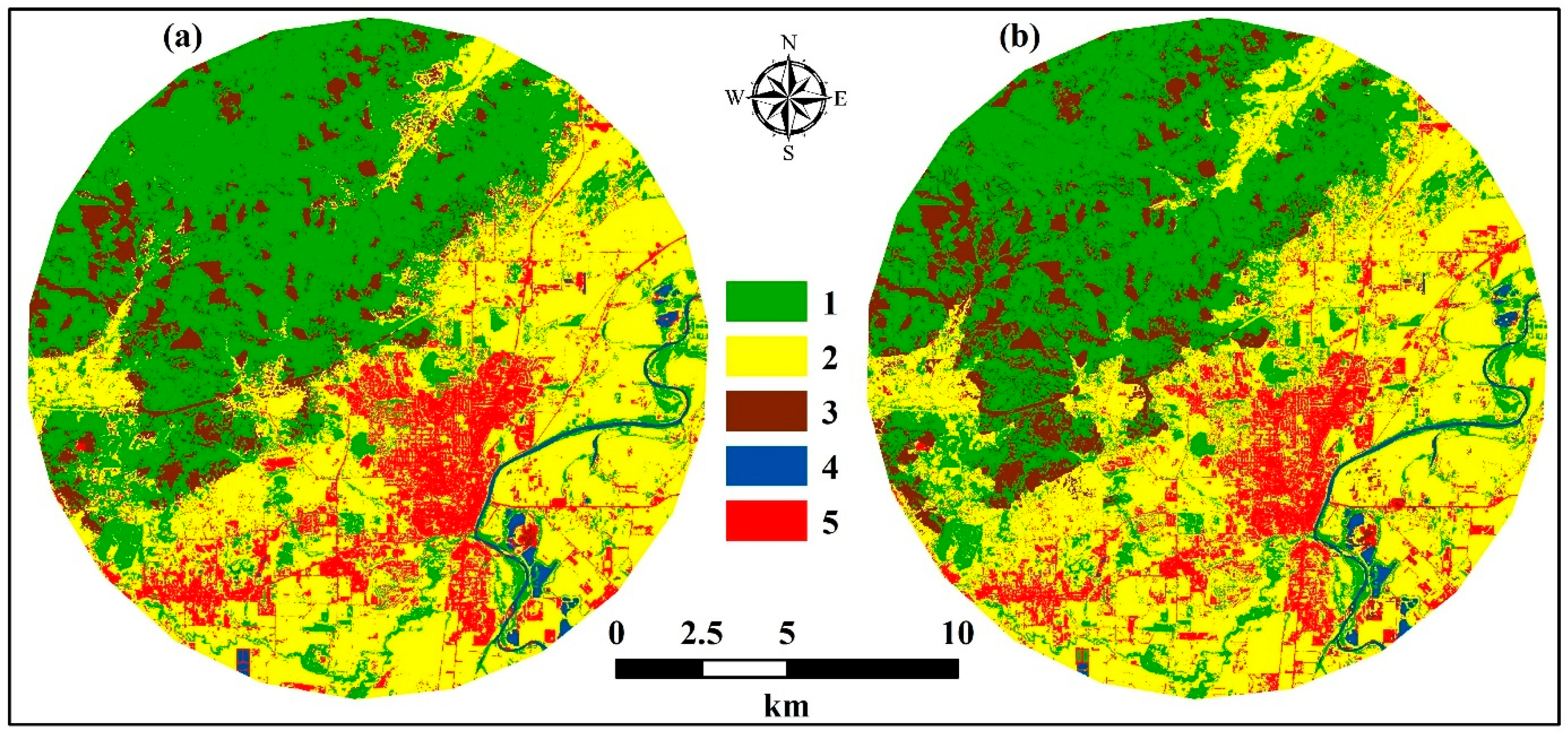
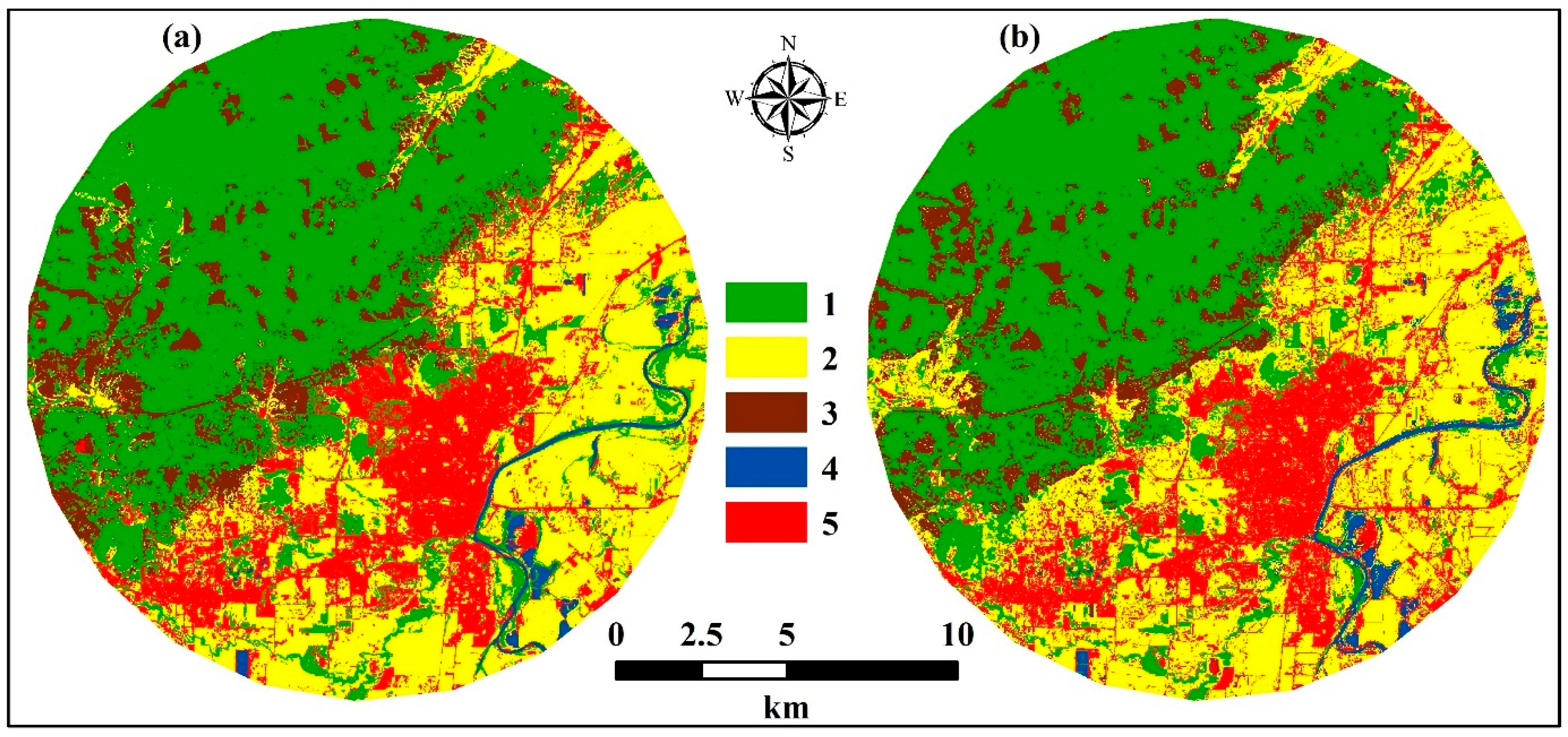
3.2. LULC Classification Maps with Elevation Data

LULC prediction maps with combinations of NDVI, NDWI, EVI, BSI, and the DEM for the study area were produced with 75 training and test data points by two methods based on machine learning techniques (Figure 8). While the CART forest class prediction result was 51.35%, the RF classification prediction decreased to 48.28%. In the agriculture class area estimation, CART was the second largest class with 39.84%. The estimate of agricultural lands increased to 40.39% with RF. This resulted in a slight increase in RF for the agricultural area estimate. The “bare soil” estimate in the CART classification was 2.48% and 5.82% with RF. The water body area estimates of CART and RF were calculated as 0.97% and 1.25%, respectively. The settlement area estimate with CART was 5.37% and RF was 4.27%. Including study area topography and the current LULC status resulted in an increase in forest and agricultural area estimates and a decrease in bare soil and settlement estimates. Additionally, the distribution of bare soil areas became more pronounced at average elevations. Classification accuracies were calculated with an overall accuracy of 85.71% and kappa of 0.82 for RF, while the overall accuracy was 76.19% and the kappa was 0.70 for CART. For the Random Forest (RF) model incorporating the DEM and spectral indices, the accuracy assessment conducted using 500 stratified random points independent of the training and testing datasets yielded an overall accuracy of 69% and a kappa coefficient of 0.62. For the CART-based LULC map generated using the DEM and indices, the overall accuracy was calculated as 77%, with a kappa value of 0.71.

The amount of training and test data was increased to 150, and the classification estimations were performed using RF and CART (Figure 9). RF estimated 41.39% of the total area as “forest”, while the CART method estimated this area lower at 35.74%. RF estimated the “agriculture” as 32.73%, while CART underestimated it as 25.13%. RF estimated the “bare soil” class as 10.38%, CART estimated it as 12.83%. While CART estimated 1.11% of the total area as “water body” class, RF estimated it as 1.05%. Thus, a very small difference emerged between the two methods for water bodies. CART estimated 25.20% of the total area as the “settlement” class, while RF estimated it as 14.46%.

The accuracy metrics for RF increased to 93.8% and the kappa value increased to 0.918. The overall accuracy and kappa value for CART was 87.5% and 0.837, respectively. As the number of datasets increased, CART increased the settlement estimate in areas covered with “bare soil” and partially “vegetation”. The CART classifier predicted the edge of the forest lands as settlement. As the training and test data numbers were increased, the RF classifier increased the density of the settlement area. For the Random Forest (RF) model incorporating the DEM and spectral indices, the accuracy assessment conducted using 500 stratified random points independent of the training and testing datasets yielded an overall accuracy of 77% and a kappa coefficient of 0.71. For the CART-based LULC map generated using the DEM and indices, the overall accuracy was calculated as 71%, with a kappa value of 0.64.

Another classification estimation was performed by increasing the dataset amount to 60 for each class with the combination of indices and DEM data (Figure 10). The total number of training and testing data for the RF and CART classifiers was increased to 300. RF estimated 41.38% of the total area as “forest”, while CART estimated this area lower at 37.96%. RF estimated the area of “agriculture” as 38.22%, while CART overestimated it as 40.31%. RF and CART estimated the “bare soil” class as 8.05% and 10.61%, respectively. Thus, CART predicted more land in the “bare soil” class than RF. RF and CART predicted the area of “water body” as 0.99% and 1.13%, respectively. CART estimated 10.13% of the area as “settlement” and RF estimated it as 11.21%. When 300 training and test points were used, the accuracy rate for RF increased to 91.46% and the kappa value increased to 0.892. The overall accuracy and kappa value for CART decreased to 87% and 0.832, respectively. For the Random Forest (RF) model incorporating the DEM and spectral indices, the accuracy assessment conducted using 500 stratified random points independent of the training and testing datasets yielded an overall accuracy of 76% and a kappa coefficient of 0.70. For the CART-based LULC map generated using the DEM and indices, the overall accuracy was calculated as 70%, with a kappa value of 0.62.

When the total number of training and testing data points for RF and CART classifiers was increased to 2500, RF estimated 45.55% of the total area as “forest” while CART estimated it as 41.49% (Figure 11). RF estimated 27.45% of the area as “agriculture” and CART estimated it as 29.90%. The RF and CART estimates of the “bare soil” class were 9.32% and 9.72%, respectively. CART estimated 1.93% of the total area to be in the “water” class, while RF estimated it as 1.37%. CART estimated 16.19% of the total area as the “settlement” class, while RF estimated it as 16.31%. The overall accuracy and the kappa value for RF increased to 98% and 0.97, respectively. The overall accuracy and the kappa value for CART decreased to 95% and 0.94, respectively. For the Random Forest (RF) model incorporating the DEM and spectral indices, the accuracy assessment conducted using 500 stratified random points independent of the training and testing datasets yielded an overall accuracy of 92% and a kappa coefficient of 0.90. For the CART-based LULC map generated using the DEM and indices, the overall accuracy was calculated as 83% with a kappa value of 0.78.

4. Discussion

We determined that the elevation data was particularly effective in correctly classifying forest types. Adding elevation information to the classification study made the terrain prediction classes of the RF classifier more balanced and realistic. The RF classifier, with elevation data added to the classification and increasing the number of test points, had an increased classification accuracy especially in bare soil estimates. The CART classifier appeared to predict a simpler and more clustered class when elevation data was added to the classification. This is evidence that the classification behavior of CART is more sensitive to variables and shows a more linear classification tendency than RF. The estimation of the water body class was not greatly affected by the addition of the DEM and the increased number of data test points. The elevation variable caused the settlement land and bare soil estimates to decrease for both methods. The overestimated classes are likely due to the lack of a subset for training and test points. Therefore, analysts should ground truth or use high-resolution images of a study area to ensure the reliability of the results from LULC classifications. Adding elevation data caused larger areas to be estimated in the forest class. CART predicted higher areas in the forest class with elevation added to the analysis when compared with RF. However, when the subset amount was increased, the forest class estimate decreased. We observed that there was an increase in the estimated areas of agricultural lands due to the effect of elevation data. The use of elevation data caused a decrease in the estimations of the bare soil class. Previous studies determined that elevation data is particularly effective in the prediction success of forest land classification and has an impact on classification accuracy [23]. The success rate of employing indices obtained from the spectral band ratio approach varied. An explanation for this is that indices more sensitive to plant reflectance values, such as NDVI, tend to produce different results in images taken during the summer, winter, and spring seasons [43]. Furthermore, since the CART classifier was sensitive to small changes in a similar investigation, RF provided more accurate LULC classifications [44].

We added a DEM to the composite of indices and increased the amount of data used for training and testing points. These varying approaches were used to examine the sensitivity of CART in classification results. The training and test data points were increased from 75 to 150, 300, and then 2500, and the field area attributes of the classification were comparatively reported (Figure 12). For the training and testing points (150 and 300) that were increased with a composition solely made up of indices, a significant discrepancy appeared in the settlement and agriculture estimations made by the CART classifier. The ranges of differences are less in the classifications produced by RF (Figure 12a–c).

The RF75 (75 training and test points), RF150, and RF300 methods showed very similar results, which indicates that these methods have similar performances. The CART150 and CART150 + DEM methods have similar performance results (Figure 12). In addition, the CART300 and CART300 + DEM methods have similar results, but they appear different from the CART results. The CART500 and CART500 + DEM methods produce similar results. In summary, while the RF methods show a more consistent and homogeneous distribution within themselves, there are more significant performance differences between the CART methods. The effect of including a DEM caused similar effects in some methods. Both the RF500 and CART500 methods appeared to have an independent performance level from other classes and the effect of DEM usage on these methods was limited. As the size of the data test points increased, a more consistent distribution appeared within the forest and agriculture land classes. For example, the “forest” class was predicted at similar rates (about 40–50%) at each realization. As the size of the data test points increased, the agriculture land estimation areas decreased. Agricultural activities could be influenced by changes across seasons. As a result, the effectiveness of identifying agricultural land was impacted by the vegetation indices that were examined.

The time required to classify the processed S2 images using the RF and CART classifiers on the GEE platform was almost the same. Other studies have determined that RF is more successful in land classification when compared with CART. However, it should be noted that the purpose of the study, dataset, decision tree levels, and study area size may cause small differences in classifier prediction success. Ref. [24] carried out fourteen different land classifications with indices and topography values for the summer and spring seasons. They reported that the elevation variable was especially effective in areas where oak species were dominant. In addition, the RF algorithm calculated a high classification with 92% overall accuracy and a 0.92 kappa value. Ref. [45] conducted a land classification study with Landsat images and reached a maximum overall accuracy of 95.2% and a maximum kappa coefficient value of 0.87 with RF. The CART results calculated a maximum overall accuracy of 89.7% with a kappa value of 0.79. In a study conducted by [46], the average overall accuracy of SVM, RF, and CART classifiers for Landsat-8 images was 90.88%, 94.85%, and 82.88%, respectively, and 93.8%, 95.8%, and 86.4% for Sentinel-2 images. These results indicate that RF classifiers outperform both SVM and CART classifiers in terms of accuracy. Ref. [47] calculated the kappa coefficients of CART and RF for Sentinel-2 images at 94% and 97%, respectively, while the average overall accuracy was 96.25%, and 98.68%, respectively. Ref. [48] analyzed Sentinel-2 and Landsat-8 images using machine learning methods by using the GEE platform for seven different years. The classification accuracy results of the study on Sentinel imagery showed that RF was more successful than CART. The overall accuracy and kappa values for RF and CART from the year 2021 were 94.42% and 0.899, and 84.62% and 0.711, respectively. Ref. [49] used two different ML algorithms for land classification with Landsat imagery. The average overall accuracy results for RF and Gradient Tree Boosting (GTB) were 96.8% and 97.1%, respectively. The kappa of RF and GTB was reported at 95.6% and 96.0%, respectively. The results revealed that GTB performed better than RF in their study. Ref. [43] examined LULC classification in a large area using Sentinel-2 and Landsat-8 datasets of Dehradun as a test case. Their results showed that RF achieved higher accuracy and kappa values compared with the CART method. For Sentinel-2 data, RF had an overall accuracy of 91.45% and a kappa value of 88.59% while CART reached an accuracy of 89.24% and a kappa value of 85.64%. In addition, the overall accuracy value of the 2019 NLCD (land cover and use model prepared with field studies and photointerpretation) study is 77.5% ± 1% for Level II classes and 83.1% ± 0.9% for Level I products [50]. In the study conducted by Lin et al. (2023) [51], a multi-level classification approach was adopted in land cover classification using both general level (e.g., broad categories such as forest, agriculture, and water) and detailed sub-classifications (e.g., coniferous forest, broadleaf forest, and rice field). The study revealed that the RF model provided high accuracy (89%) for the first level (general classes), while a decrease in accuracy rates was observed (79%) due to the increase in similarities between classes in more detailed sub-classes (second and third levels). In a similar study, Kadri et al. (2023) [52], using the RF model, demonstrated high classification success with 96–99% overall accuracy and 0.93–0.98 kappa coefficient on training and testing data. In addition, validation with independent ground control points increased the reliability of the results by supporting the spatial validity of the model. In this study, the overall accuracy of RF reached 90% and above. The variables contributing to these accuracy differences are likely (1) the temporal and spatial resolution of the satellite imagery, (2) the reduced size and management practices of the study area, (3) the smaller diversity in land classes, and (4) the classification methods. Kappa values and overall accuracy are typically higher in small datasets (15–30 samples per class). Therefore, it is difficult to conclusively evaluate the success of our results. It is possible that classification performance could be explained in more detail with metrics such as Quantity Disagreement and Allocation Disagreement [53]. Considering our results, future research could integrate higher-resolution images or time series to improve classification accuracy over heterogeneous landscapes. Additionally, the machine learning framework implemented here could be tested in different ecological zones to assess its transferability and robustness. In addition, it has been shown that integrating local knowledge is a powerful tool in understanding the cause of changes [52]. Past, current, and future LULC research has high potential for use in cloud computing with machine learning techniques supported by multi-disciplinary studies [54].

5. Conclusions

We made land classification estimates using data representing five land cover categories. In the study area, the largest area was forest cover, followed by agricultural land, residential areas, bare soil, and water bodies. Considering the size of the area, both classifiers showed classification success within reasonable ranges despite using a small number of data test points. However, the RF classifier came to the fore in LULC class estimation. CART showed high sensitivity to the smallest change (height, number of data test points, and rate). When the amount of training points was decreased, the elevation variable became more effective in the classification results. The use of elevation data was also effective in determining forest openings. We recommend that both RF and CART’s bare soil and settlement land class estimation results could be evaluated more thoroughly and that the appropriate number of training and test data points could be further investigated. According to the data and techniques used in this study, the least affected class was the water body estimations. RF was successful in estimating forest and agricultural lands more effectively than CART. The obtained accuracy metrics indicated that the ensemble-based RF approach was more robust and accurate than the CART algorithm. Increasing the data test points was not very effective in estimating the water body class in the study area. However, as the data test points increased, the accuracies increased in estimating settlement land. Platforms that combine cloud computing and deep learning techniques can undoubtedly save time over ground-based data collection approaches in land classification. In future studies, more advanced techniques and compositions for forestry could be investigated by adding slope, aspect, and stand type maps as data. RS and cloud-based analysis have the potential to be an effective method in sustainable land management and environmental planning processes.

References

1. Tin, D.; Cheng, L.; Le, D.; Hata, R.; Ciottone, G. Natural disasters: A comprehensive study using EMDAT database 1995–2022. Public Health 2024, 226, 255–260. [Google Scholar] [CrossRef] [PubMed]
2. Daimon, H.; Miyamae, R.; Wang, W. Navigating theories of actions on disaster prevention: A systematic review on disaster research in Japan. Nat. Hazards Rev. 2023, 24, 03123002-1–03123002-15. [Google Scholar] [CrossRef]
3. Pratiti, R. An ecological approach to disaster mitigation: A literature review. Cureus 2023, 15, e45500. [Google Scholar] [CrossRef] [PubMed]
4. Gómez, C.; White, J.C.; Wulder, M.A. Optical remotely sensed time series data for land cover classification: A review. ISPRS J. Photogramm. Remote Sens. 2016, 116, 55–72. [Google Scholar] [CrossRef]
5. Loveland, T.R.; Reed, B.C.; Brown, J.F.; Ohlen, D.O.; Zhu, Z.; Yang, L.; Merchant, J.W. Development of a global land cover characteristics database and IGBP DISCover from 1 km AVHRR data. Int. J. Remote Sens. 2000, 21, 1303–1330. [Google Scholar] [CrossRef]
6. Khan, S.M.; Shafi, I.; Butt, W.H.; Diez, I.D.L.T.; Flores, M.A.L.; Galán, J.C.; Ashraf, I. A systematic review of disaster management systems: Approaches, challenges, and future directions. Land 2023, 12, 1514. [Google Scholar] [CrossRef]
7. Scheffer, M.; Carpenter, S.; Foley, J.A.; Folke, C.; Walker, B. Catastrophic shifts in ecosystems. Nature 2001, 413, 591–596. [Google Scholar] [CrossRef]
8. Hahn, W.A.; Knoke, T. Sustainable development and sustainable forestry: Analogies, differences, and the role of flexibility. Eur. J. For. Res. 2010, 129, 787–801. [Google Scholar] [CrossRef]
9. Gorelick, N.; Hancher, M.; Dixon, M.; Ilyushchenko, S.; Thau, D.; Moore, R. Google Earth Engine: Planetary-scale geospatial analysis for everyone. Remote Sens. Environ. 2017, 202, 18–27. [Google Scholar] [CrossRef]
10. Zhao, Q.; Yu, L.; Li, X.; Peng, D.; Zhang, Y.; Gong, P. Progress and trends in the application of Google Earth and Google Earth Engine. Remote Sens. 2021, 13, 3778. [Google Scholar] [CrossRef]
11. Benhammou, Y.; Alcaraz-Segura, D.; Guirado, E.; Khaldi, R.; Achchab, B.; Herrera, F.; Tabik, S. Sentinel2GlobalLULC: A Sentinel-2 RGB image tile dataset for global land use/cover mapping with deep learning. Sci. Data 2022, 9, 681. [Google Scholar] [CrossRef]
12. Talukdar, S.; Singha, P.; Mahato, S.; Shahfahad; Pal, S.; Liou, Y.-A.; Rahman, A. Land-use land-cover classification by machine learning classifiers for satellite observations—A review. Remote Sens. 2020, 12, 1135. [Google Scholar] [CrossRef]
13. Gülci, S.; Gülci, N.; Yüksel, K. Monitoring water surface area and land cover change by using Landsat imagery for Aslantas Dam Lake and its vicinity. J. Inst. Sci. Technol. 2019, 9, 100–110. [Google Scholar] [CrossRef]
14. Gülci, S.; Yüksel, K.; Gümüş, S.; Wing, M. Mapping Wildfires Using Sentinel 2 MSI and Landsat 8 Imagery: Spatial Data Generation for Forestry. Eur. J. For. Eng. 2021, 7, 57–66. [Google Scholar] [CrossRef]
15. Tamiminia, H.; Salehi, B.; Mahdianpari, M.; Quackenbush, L.; Adeli, S.; Brisco, B. Google Earth Engine for geo-big data applications: A meta-analysis and systematic review. ISPRS J. Photogramm. Remote Sens. 2020, 164, 152–170. [Google Scholar] [CrossRef]
16. Farhadi, H.; Najafzadeh, M. Flood risk mapping by remote sensing data and random forest technique. Water 2021, 13, 3115. [Google Scholar] [CrossRef]
17. Amani, M.; Mahdavi, S.; Afshar, M.; Brisco, B.; Huang, W.; Mohammad Javad Mirzadeh, S.; Hopkinson, C. Canadian wetland inventory using Google Earth Engine: The first map and preliminary results. Remote Sens. 2019, 11, 842. [Google Scholar] [CrossRef]
18. Lobo, F.D.L.; Souza-Filho, P.W.M.; Novo, E.M.L.D.M.; Carlos, F.M.; Barbosa, C.C.F. Mapping mining areas in the Brazilian amazon using MSI/Sentinel-2 imagery (2017). Remote Sens. 2018, 10, 1178. [Google Scholar] [CrossRef]
19. Senay, G.B.; Friedrichs, M.; Morton, C.; Parrish, G.E.; Schauer, M.; Khand, K.; Huntington, J. Mapping actual evapotranspiration using Landsat for the conterminous United States: Google Earth Engine implementation and assessment of the SSEBop model. Remote Sens. Environ. 2022, 275, 113011. [Google Scholar] [CrossRef]
20. Franklin, S.E.; Dickson, E.E.; Hansen, M.J.; Farr, D.R.; Moskal, L.M. Quantification of landscape change from satellite remote sensing. For. Chron. 2000, 76, 877–886. [Google Scholar] [CrossRef]
21. Agdas, M.G.; Yenen, Z. Determining land use/land cover (LULC) changes using remote sensing method in Lüleburgaz and LULC change’s impacts on SDGs. Eur. J. Sustain. Dev. 2023, 12, 1–24. [Google Scholar] [CrossRef]
22. Lawrence, R.L.; Wright, A. Rule-based classification systems using classification and regression tree (CART) analysis. Photogramm. Eng. Remote Sens. 2001, 67, 1137–1142. [Google Scholar]
23. Gislason, P.O.; Benediktsson, J.A.; Sveinsson, J.R. Random forests for land cover classification. Pattern Recognit. Lett. 2006, 27, 294–300. [Google Scholar] [CrossRef]
24. Rodriguez-Galiano, V.F.; Ghimire, B.; Rogan, J.; Chica-Olmo, M.; Rigol-Sanchez, J.P. An assessment of the effectiveness of a random forest classifier for land-cover classification. ISPRS J. Photogramm. Remote Sens. 2012, 67, 93–104. [Google Scholar] [CrossRef]
25. Pande, C.B.; Srivastava, A.; Moharir, K.N.; Radwan, N.; Mohd Sidek, L.; Alshehri, F.; Zhran, M. Characterizing land use/land cover change dynamics by an enhanced random forest machine learning model: A Google Earth Engine implementation. Environ. Sci. Eur. 2024, 36, 84. [Google Scholar] [CrossRef]
26. Phan, T.N.; Kuch, V.; Lehnert, L.W. Land cover classification using google earth engine and random forest classifier—The role of image composition. Remote Sens. 2020, 12, 2411. [Google Scholar] [CrossRef]
27. European Space Agency (ESA). Sentinel-2 MSI: MultiSpectral Instrument, Level-2A. Available online: https://s2.pages.eopf.copernicus.eu/pdfs-adfs/MSI/L2/PDFS_S2_MSI_L2.myst.html (accessed on 22 June 2025).
28. Google Earth Engine Team. Google Earth Engine: A Planetary-Scale Geospatial Analysis Platform. Available online: https://earthengine.google.com (accessed on 12 January 2025).
29. Farr, T.G.; Rosen, P.A.; Caro, E.; Crippen, R.; Duren, R.; Hensley, S.; Kobrick, M.; Paller, M.; Rodriguez, E.; Roth, L.; et al. The shuttle radar topography mission. Rev. Geophys. 2007, 45, RG2004. [Google Scholar] [CrossRef]
30. USGS. SRTMGL1 v003 NASA Shuttle Radar Topography Mission Global 1 Arc Second. Available online: https://lpdaac.usgs.gov/products/srtmgl1v003/ (accessed on 16 December 2024).
31. Tucker, C.J. Red and photographic infrared linear combinations for monitoring vegetation. Remote Sens. Environ. 1979, 8, 127–150. [Google Scholar] [CrossRef]
32. Huete, A.R.; Liu, H.Q.; Batchily, K.; van Leeuwen, W. A comparison of vegetation indices global set of TM images for EOS-MODIS. Remote Sens. Environ. 1997, 59, 440–451. [Google Scholar] [CrossRef]
33. Huete, A.; Didan, K.; Miura, T.; Rodriguez, E.P.; Gao, X.; Ferreira, L.G. Overview of the radiometric and biophysical performance of the MODIS vegetation indices. Remote Sens. Environ. 2002, 83, 195–213. [Google Scholar] [CrossRef]
34. Wu, C.; Chen, J.M.; Huang, N. Predicting gross primary production from the enhanced vegetation index and photosynthetically active radiation: Evaluation and calibration. Remote Sens. Environ. 2011, 115, 3424–3435. [Google Scholar] [CrossRef]
35. McFeeters, S.K. The use of the normalized difference water index (NDWI) in the delineation of open water features. Int. J. Remote Sens. 1996, 17, 1425–1432. [Google Scholar] [CrossRef]
36. Breiman, L. Random forests. Mach. Learn. 2001, 45, 5–32. [Google Scholar] [CrossRef]
37. Breiman, L.; Friedman, J.H.; Olshen, R.A.; Stone, C.J. Classification and Regression Trees, 1st ed.; Chapman and Hall/CRC: New York, NY, USA, 1984; pp. 1–368. [Google Scholar] [CrossRef]
38. GEE. The “Classifier” Package Handles Supervised Classification by Traditional ML Algorithms Running in Earth Engine. Available online: https://developers.google.com/earth-engine/guides/classification (accessed on 2 February 2025).
39. Cohen, J. A coefficient of agreement for nominal scales. Educ. Psychol. Meas. 1960, 20, 37–46. [Google Scholar] [CrossRef]
40. Stehman, S.V. Selecting and interpreting measures of thematic classification accuracy. Remote Sens. Environ. 1997, 62, 77–89. [Google Scholar] [CrossRef]
41. Congalton, R.G.; Green, K. Assessing the Accuracy of Remotely Sensed Data: Principles and Practices, 2nd ed.; CRC Press: Boca Raton, FL, USA, 2008; pp. 1–200. [Google Scholar] [CrossRef]
42. Foody, G.M. Impacts of ignorance on the accuracy of image classification and thematic mapping. Remote Sens. Environ. 2021, 259, 112367. [Google Scholar] [CrossRef]
43. Srivastava, A.; Bharadwaj, S.; Dubey, R.; Sharma, V.B.; Biswas, S. Mapping vegetation and measuring the performance of machine learning algorithm in LULC classification in the large area using Sentinel-2 and Landsat-8 datasets of Dehradun as a test case. Int. Arch. Photogramm. Remote Sens. Spat. Inf. Sci. 2022, 43, 529–535. [Google Scholar] [CrossRef]
44. Yimer, S.M.; Bouanani, A.; Kumar, N.; Tischbein, B.; Borgemeister, C. Comparison of different machine-learning algorithms for land use land cover mapping in a heterogenous landscape over the Eastern Nile River basin, Ethiopia. Adv. Space Res. 2024, 74, 2180–2199. [Google Scholar] [CrossRef]
45. Zafar, Z.; Zubair, M.; Zha, Y.; Fahd, S.; Nadeem, A.A. Performance assessment of machine learning algorithms for mapping of land use/land cover using remote sensing data. Egypt. J. Remote Sens. Space Sci. 2024, 27, 216–226. [Google Scholar] [CrossRef]
46. Loukika, K.N.; Keesara, V.R.; Sridhar, V. Analysis of land use and land cover using machine learning algorithms on google earth engine for munneru river basin, India. Sustainability 2021, 13, 13758. [Google Scholar] [CrossRef]
47. Zhao, Z.; Islam, F.; Waseem, L.A.; Tariq, A.; Nawaz, M.; Islam, I.U.; Hatamleh, W.A. Comparison of three machine learning algorithms using google earth engine for land use land cover classification. Rangel. Ecol. Manag. 2024, 92, 129–137. [Google Scholar] [CrossRef]
48. Arpitha, M.; Ahmed, S.A.; Harishnaika, N. Land use and land cover classification using machine learning algorithms in google earth engine. Earth Sci. Inform. 2023, 16, 3057–3073. [Google Scholar] [CrossRef]
49. Ayalke, G.Z.; Şişman, A. Machine learning-based improved land cover classification using Google Earth Engine: Case of Atakum, Samsun. Geomatik 2024, 9, 375–390. [Google Scholar] [CrossRef]
50. Wickham, J.; Stehman, S.V.; Sorenson, D.G.; Gass, L.; Dewitz, J.A. Thematic accuracy assessment of the NLCD 2019 land cover for the conterminous United States. GIScience Remote Sens. 2023, 60, 2181143. [Google Scholar] [CrossRef]
51. Lin, C.; Doyog, N.D. Challenges of retrieving LULC information in rural-forest mosaic landscapes using random forest technique. Forests 2023, 14, 816. [Google Scholar] [CrossRef]
52. Kadri, N.; Jebari, S.; Augusseau, X.; Mahdhi, N.; Lestrelin, G.; Berndtsson, R. Analysis of four decades of land use and land cover change in semiarid Tunisia using Google Earth Engine. Remote Sens. 2023, 15, 3257. [Google Scholar] [CrossRef]
53. Pontius, R.G.; Millones, M. Death to Kappa: Birth of quantity disagreement and allocation disagreement for accuracy assessment. Int. J. Remote Sens. 2011, 32, 4407–4429. [Google Scholar] [CrossRef]
54. Abdelsamie, E.A.; Mustafa, A.-r.A.; El-Sorogy, A.S.; Maswada, H.F.; Almadani, S.A.; Shokr, M.S.; El-Desoky, A.I.; Meroño de Larriva, J.E. Current and potential land use/land cover (LULC) scenarios in dry lands using a CA-Markov simulation model and the Classification and Regression Tree (CART) method: A cloud-based Google Earth Engine (GEE) approach. Sustainability 2024, 16, 11130. [Google Scholar] [CrossRef]
Figure 1. Mosaic of Sentinel-2 red, green, and blue (RGB) images and the spatial distribution of 75 training and test datasets in the study area.
Geomatics 05 00029 g001
Figure 2. Visible S2 bands composites (a), DEM (b), NDVI (c), NDWI (d), EVI (e), and BSI (f) for the study area.
Geomatics 05 00029 g002
Figure 3. GEE code editor interface and the spatial distribution of 75 (a), 150 (b), 300 (c), and 2500 (d) training and testing datasets. (Each colored pinpoint represents a LULC class: forest is green, agriculture is yellow, bare soil is purple, water is blue, and settlement is red).
Geomatics 05 00029 g003
Figure 4. Classification maps of RF (a) and CART (b) created using 75 training and test data points for composite indices.
Geomatics 05 00029 g004
Figure 5. Classification maps of RF (a) and CART (b) created using 150 training and test data points for composite indices.
Geomatics 05 00029 g005
Figure 6. Classification maps of RF (a) and CART (b) created using 300 training and test data points for composite indices.
Geomatics 05 00029 g006
Figure 7. Classification maps of RF (a) and CART (b) created using 2500 training and test data points for composite indices.
Geomatics 05 00029 g007
Figure 8. Classification maps of RF (a) and CART (b) created using 75 training and test data points for composite indices and DEM.
Geomatics 05 00029 g008
Figure 9. Classification maps of RF (a) and CART (b) created using 150 training and test data points for composite indices and DEM.
Geomatics 05 00029 g009
Figure 10. Classification maps of RF (a) and CART (b) created using 300 training and test data points for composite indices and DEM.
Geomatics 05 00029 g010
Figure 11. Classification maps of RF (a) and CART (b) created using 2500 training and test data points for composite indices and DEM.
Geomatics 05 00029 g011
Figure 12. The heatmap presents the area (%) information of LULC classes for 75 (a), 150 (b), 300 (c), and 2500 (d) training and test points.
Geomatics 05 00029 g012