Review of the Problem of the Earth Shape

Abstract

The determination of the shape of the Earth has been one of the fundamental problems geodesy was supposed to solve; it has been and possibly still is the main geodetic problem. It is thus appropriate for geodesists to look at this problem periodically, and this is what the authors of this paper aim to do. About 50 years ago, geodesists started using satellites as a new and very powerful tool. Many problems that were either impossible to solve or that presented almost unsurmountable hurdles to solutions have now been solved relatively simply, so much so that in the eyes of some people, satellites can solve all geodetic problems, and attempts are being made to show that this is indeed the case. We feel that the time has come to show that even satellites have their limitations, the main one being that for them to remain in their orbit, they must fly quite high, typically at several hundred kilometres. The gravitational field of the Earth (and that of any celestial body) smoother as one gets higher and higher. In other words, the gravitational field at the satellite orbit altitude loses detailed information that one can see at the surface of the Earth. In this contribution, we shall try to explain what satellites have contributed to the study of the shape of the Earth and what issues remain to be sorted out.

1. Historical Perspective

The term “Shape of the Earth” has had different meanings since it was first realized that it would be good to understand this particular property of the Earth, probably about 1000 years BC. The first real attempt to discuss the shape of the Earth dates back to Aristotle, to about 350 BC.

(1)

The first experiment to determine the size of the Earth, considered to be a sphere (as part of a geocentric Ptolemaic system described later in Hypotheseis tōn planōmenōn or Planetary Hypotheses) was conducted by Claudius Ptolemy (100–170 AD) in Egypt [1]. The Ptolemaic estimate was about 18% too small. Eratosthenes’ estimate, made a bit later, was probably accurate to 1–2%. The idea of a spherical Earth remained valid until the eighteenth century. A proof of this is the Globus cruciger, a Christian symbol of authority, in which the Earth is represented by an orb bearing a cross; see Figure 1.

(2)

The next step was the adoption of an ellipsoid of revolution after a French versus English dispute over whether the ellipsoid was oblate or prolate was won by Newton. The official measurement of the size of the Earth was carried out under the auspices of the French Academy of Science in the period 1792 to 1799, assuming the flattening to be 1/308.6 instead of the correct value of 1/298.257 [2].

(3)

The next estimate occurred more quickly this time and was made by the German geodesist Carl Friedrich Gauss, who suggested using the equipotential surface of the Earth gravity field as a more realistic Earth shape [3]. The equipotential surface he had in mind was the one that was supposed to follow the mean sea level, as this would represent the Earth shape well over the oceans, which was later named the geoid by Gauss’s student Listing [4].

(4)

Now, we can deal with the physical surface of the Earth as the most realistic representation of the shape of the Earth on dry land. Over the oceans, the geoid may still be the best representation of the Earth.

2. Geometrical Aspects

Let us concentrate first on the problems encountered with the ellipsoid of revolution. This ellipsoid is also called biaxial (to distinguish it from the triaxial ellipsoid that some geodesists were unsuccessfully trying to introduce instead of the ellipsoid of revolution) or the geodetic reference ellipsoid because of its role in the description of the other two much more irregular surfaces, the geoid and the physical surface of the Earth. The geodetic reference ellipsoid is defined by two parameters, the semi-major axis a and the semi-minor axis b or alternatively by a and the flattening f:

$$f={\displaystyle \frac{a-b}{a}}.$$

(1)

Other pairs of parameters are sometime used. The geodetic coordinate system [5] (p. 324) $(\phi ,\lambda ,h)$, where $\phi$ is the geodetic latitude, $\lambda$ is the geodetic longitude, and h is the geodetic height, is defined vis-à-vis the geodetic reference ellipsoid in such a way that $(\phi ,\lambda )$, referred to as $\mathsf{\Omega }$, are the curvilinear horizontal coordinates on the ellipsoid and h is reconned from the geodetic reference ellipsoid, up in the direction normal to the ellipsoid. Clearly, the coordinate system is ellipsoidal, but it was specifically designed for geodetic uses, hence the name “geodetic”. The geodetic coordinate system is clearly a purely geometrical quantity.

Successive geodetic reference ellipsoids have been introduced through international acclamations. The “French” ellipsoid mentioned earlier was accepted at the beginning of the 19th century following the recommendation by the French Academy of Science as part of their attempt to introduce the Système international d’unités (International System of Units). The size and shape of the Earth were to be the basis for the universally used length system: one metre was to be and still is supposed to be, according to the original definition, a ten-millionth part of the Earth quadrant, understood at the time of the definition’s acceptance as a quadrant of the best-fitting ellipsoid to the shape of the Earth. As a remark, let us mention that this accepted metre is short by 200 μm. While the French measurement conducted at the end of the 18th century was good to 4 μm, the subsequent calculations were wrong because of their lack of knowledge of Earth’s gravity field [6].

The reference ellipsoid (biaxial and geocentric) is defined as a part of the Geodetic Reference System. Its latest version, called Geodetic Reference System 1980, was adopted by the International Association of Geodesy (IAG) in 1979 [7]. Its biaxial ellipsoid has its major semi-axis a defined by the mean equatorial radius of the Earth, 6,378,137 m, and its inverse value of flattening is 298.257222101. Such an ellipsoid fitted to a sphere of radius a would be 21.385 km short of the radius of that sphere at the poles.

We should, perhaps, mention that even though the geodetic reference ellipsoid is a purely geometrical construction, it was shown by Pizzeti [8] and Somigliana [9] that it can also be considered an equipotential surface of the normal gravity field [10] (Section 2-8) and thus the normal shape of the geoid as well, giving it some physical meaning. We will not use this feature of the geodetic reference ellipsoid directly in this contribution. Geodetic heights are of little use in practice [11], as we can appreciate from Figure 2.

Even for other uses, besides the shape of the Earth, the need for a physically meaningful system exists because physics must not be neglected and any applications, for instance, engineering applications, will have to take physics into account. Let us just mention here that it was impossible to measure geodetic coordinates directly before the appearance of satellites, i.e., say, 50 years ago.

3. Physical Aspects

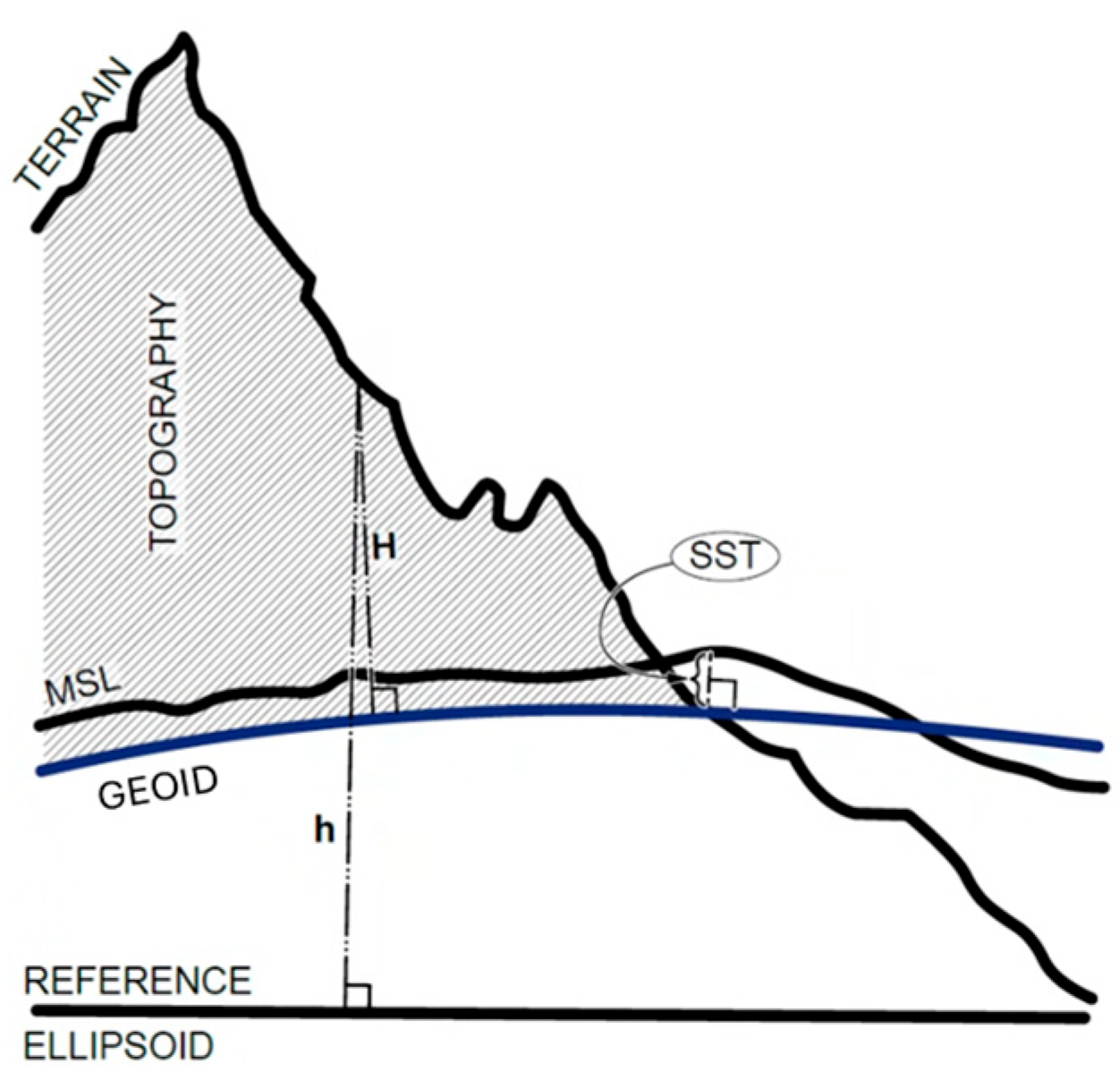
The geoid is a purely physical surface (an equipotential surface of the Earth gravity field that is convex everywhere) referred to the reference ellipsoid by geodetic heights called geoidal heights (denoted by N), which can be positive or negative depending on whether the point of interest is above or below the surface of the reference ellipsoid, respectively. It is possibly the most important surface in geodesy as it is one of the forms of the Earth’s shape and, at the same time, a reference surface for physically meaningful heights. The (constant) gravity potential on the geoid is chosen so that the geoid (surface) is globally as close as possible to the mean sea level (MSL), determined from tide gauge measurements and sea surface altimetry over a “long period of time”. This global mission is a difficult one; consequently, the links to the MSL are the weakest links yet in the determination of the shape of the Earth. In principle, measurements of the instantaneous sea level by tide gauges and satellite altimetry (with radio waves and other instruments used to measure sea level heights globally) are corrected for all known dynamic and other effects responsible for the fact that the real sea level is not really level, i.e., does not follow an equipotential surface, and averaged over time to obtain the mean sea level (mean for the span of available data). Geoidal heights, N (if we were to follow the misapprehension in geodesy of calling the “geodetic height” “ellipsoidal height”, we would have to call them “ellipsoidal heights of the geoid”, which just shows another reason why the term “ellipsoidal heights” should NOT be used), range roughly between −100 and +100 metres. Let us just mention the fact that the geoid, being an equipotential surface of the Earth’s gravity field, varies in time. The variations are minute (millimetres per year), but when talking about it as the surface representing the shape of the Earth, its temporal changes should be considered. So far, this problem has not been dealt with in practice.

Physically meaningful (practical) heights, called orthometric [10] (Section 4-4), are referred to the geoid; i.e., points on the geoid have an orthometric height equal to 0. Orthometric (ortho means straight, upright, correct) height is the distance between the point of interest and the geoid measured along the plumbline that goes through the point of interest, measured with an exact metre yardstick; it is a Euclidean metric. This length is indistinguishable from the length of the straight line connecting the point of interest to the intersection of the plumbline with the geoid; see, e.g., [12]. This line is, for all intents and purposes, orthogonal to the geoid. The remarks about the temporal variations of the geoid given at the end of the immediately preceding paragraph are even more applicable to orthometric heights, as these variations are much larger than those of the geoid.

Orthometric heights are determinable from terrestrial levelling measurements. Levelling lines connect the points of interest to the “datum points for physical heights”, measured with tide gauges where the sea level has been observed for a long time. At these points, the orthometric height of the MSL above the geoid, called, predictably, “Sea Surface Topography” (SST), should be known to enable us to associate the orthometric heights with the geoid rather than with the MSL, but, as stated above, this is the weakest link yet in the process of the determination of the Earth’s shape. The most accurate orthometric heights must be obtained considering the effect of the gravity field, as the orthometric heights are heights that are based on physical (understand gravitational) laws. Not many countries have orthometric heights based on sound gravitational principles, and those countries that do not, use a simple approximative approach introduced by Helmert in [13]. The accuracy of Helmert’s approximate orthometric heights is within a few decimetres. These approximate heights can and should be converted into rigorous orthometric heights following the procedures described in [14], which improve the accuracy of orthometric heights by one order of magnitude. Orthometric heights determined by levelling thus lead to high costs as well as an unwelcome accumulation of errors; see, e.g., [15]. But before the appearance of geodetic satellites, some 50 years ago, there was no other way of measuring them. With the appearance of navigation satellites, it became possible to measure the 3D positions of points on and above the Earth surface directly. Thus, geodetic heights became determinable, relatively cheaply and accurately. But, as mentioned above, geodetic heights are of little use in practice. For practical applications and for the determination of the actual (physical) shape of the Earth, it is necessary to convert the geodetic heights to orthometric heights, which is carried out by the “basic congruency equation”, an equation that makes sure that geodetic and orthometric heights can be transformed back and forth freely. In other words, the geodetic height system (geometric) is congruent with the physical terrestrial height system. Or, in other words, the existing height system based on terrestrially determined orthometric heights is congruent with the modern geometrical, satellite-based geodetic system of heights.

The basic congruency Equation (2) is a more complete version of Equation (3) from [11], with the difference being that SST(Ω), the orthometric height (above the geoid) of the mean sea level (MSL), makes an appearance here as the link between the real datum of orthometric heights (geoid) and the datum of terrestrially observed orthometric heights (MSL):

$$H_{ter}\left(\mathsf{\Omega }\right)+SST\left(\mathsf{\Omega }\right)=h\left(\mathsf{\Omega }\right)-N\left(\mathsf{\Omega }\right),$$

(2)

where $H_{ter}$ is the orthometric height determined by terrestrial observations, referred to the MSL. (Let us mention that the source quoted here does not mean that the authors were the first ones to formulate the equation.) We have already defined the geodetic height h and orthometric height H. The other two quantities, the Sea Surface Topography, SST, also known as the dynamic ocean topography, and geoidal heights, N, are of a physical nature, and their accurate determination is somewhat more challenging than the purely geometrical determination of geodetic heights.

4. Physical Problems Encountered

The SST represents the highs and lows of the mean ocean surface relative to the geoid; see Figure 3. It is estimated by satellite altimeters, which measure the distance from the sensor in orbit to the surface of the water. The satellite’s altitude is taken with respect to the reference ellipsoid using their positions estimated by onboard GNSS receivers. The SST is routinely estimated within an accuracy of a few centimetres by several institutions around the world. However, there is currently no international service that could coordinate these efforts and/or combine individual solutions and produce one official product, as is the case with the geoid (International Geoid Service) or the Earth’s gravitational field (International Gravity Field Service). To the best of our knowledge, the biggest contribution to the SST is due to the permanent difference of the (average) temperature, and thus density, of oceanic waters between the polar and equatorial regions, which lowers the mean sea level in polar regions by about 1.5 m and adds 1.5 m to the mean level in equatorial regions. It should be clear that N($\mathsf{\Omega })$ + SST($\mathsf{\Omega })$ describes the MSL with respect to the reference ellipsoid, which is, possibly, an even better representation of the physical shape of the Earth over the oceans than the geoid. The accuracy of the SST term changes from place to place, depending on how many orthometric datum points have been used in the establishment of the local/regional terrestrial levelling networks. If only one datum point was used in the country, or in the wider region, then we are talking about just one number, but if there are more datum points used, the situation will get more complicated.

Geoidal heights can be determined nowadays to a sub centimetre accuracy in a region of modest elevation (up to 2000 m) if the observed gravity data, topographic elevations, and topographic density variations are known to a reasonable spatial resolution and accuracy [16]. Though it has to be emphasized that the approach to geoid determination, such as the one described in [16], has to follow rigorous physical principles. But, of the four quantities that appear in the basic congruency equation (Equation (2)), the geoidal height can now probably be determined the most accurately. The accuracy of geodetic heights, as measured by GNSS, is about 2 cm, while the accuracy of orthometric heights obtained from levelling is about 2 to 3 cm in a region of good geodetic coverage, such as Europe and North America [17].

This is probably a good place to mention an alternative height system, invented by Russian geodesist M.S. Molodensky [18], that is now being used in some countries. Molodensky’s approach does not use the geoid, neither as one of the shapes of the Earth nor as a reference surface for heights, but uses a non-physical surface called the quasi-geoid instead; see Figure 4.

This surface is not suitable for any application as it contains folds, corners, edges, and shapes that are not easy to work with mathematically [11]. And quasigeoid has no physical meaning at all. But Molodensky’s heights can be, and are being, used in an alternative way, in which case they are called normal heights. They may be referred to the geoid, but the price one pays for using this alternative is that the magnitude of the normal height is not measured by a Euclidean metric. This is why we do not talk about these heights in this paper.

As we are reviewing here also height systems other than the orthometric heights, it is probably justified to mention dynamic heights as well. They should be included in this presentation as they should be of interest to people who use heights to solve physical problems rather than being interested in the shape of the Earth as such. The difference between orthometric and dynamic heights is that orthometric heights are measured in fixed metres while dynamic heights are measured on a scale varying according to gravity force, which changes from place to place. Thus, a lake water level (above the sea level) expressed as an orthometric height will show that the water level does not have the same height everywhere, even though the mean lake level follows an equipotential surface as physics requires it to do. In other words, orthometric heights, by using a fixed metric, give us a geometrical view of reality when portraying the shape of the Earth and not an understanding of the physical laws in action. If we want to use heights that reflect the physical laws in action above the geoid, we must go for dynamic heights [5] (Section 4-5), which use a metric that changes with location. When referring to dynamic heights here, we are talking about drainage, irrigation, sea level rise or fall, and other geodynamical applications and not about the physical surface of the Earth.

In any case, as far as the shape of the Earth is concerned, it appears now that the geoid can be determined most accurately if a reasonable topographical mass density, as well as other data (e.g., gravity anomaly, digital terrain model), is available. The recent work of [19] has contributed a great deal to the availability of a global lateral topographical mass density distribution and thus contributed to the accuracy of geoid determination, as well as the improvement in the accuracy of orthometric heights. As databases are being improved daily, we should mention the recent availability of airborne gravimetry and the abundance of data that comes from it [20]. The hope is that soon orthometric heights will become determinable to sufficient accuracy so that even the real shape of the solid Earth can be determined to an accuracy compatible with the accuracy of the geoid.

In the derivation of the geoid, the two main data sources are terrestrial gravity observations and the satellite-observed gravity. The former are available as point observations, and the latter are more often used in the form of computed coefficients in spherical harmonic series representations of the gravitational potential [10] (Equation 1-54); the data are therefore dealt with in a spatial manner and spectral manner, respectively. It is known that spatial expressions can be transformed to equivalent spectral expressions and vice versa at any stage. But it should be understood that spectral representations (global solutions expressed in series form) are the most suitable form to use in global applications, while spatial representations are more suitable for local/regional representations, which are usually more accurate.

The real problem with global (satellite-only) solutions for the gravitational field is that the gravitational field becomes smoother and smoother as one gets further away from the attracting masses. At the height of satellite orbits, higher measured frequency constituents are either too noisy (and thus filtered out) or at least attenuated sufficiently so that they are not observable at those satellite heights. Thus, satellite global solutions have a natural physical upper limit of validity in terms of frequencies and thus cannot be used to an arbitrarily high degree of harmonic series. Thus, global satellite solutions are excellent and necessary for long-wavelength constituents, but they have a physical validity limit at high frequencies. If providers wish to present degrees higher than those supported by collected satellite data, they must use also terrestrial observations in one form or another.

Smoothing of the field works according to the horizontal extent of the feature (the bump, the wave amplitude); the smaller the horizontal extent of the feature, the faster it is going to disappear with height. This is usually formulated in terms of the “attenuation factor” (a function of frequency—degree n, the reciprocal of the feature’s horizontal extent, and the height h of the equipotential surface), whose shape is of interest. The attenuation factor, derived from [5] (Equation 20.44), when we look at the changes in the radial function [a/(a + h)]ⁿ with heigh h, reads

$$f\left(n,h\right)={\left({\displaystyle \frac{1}{1+\raisebox{1ex}{$h$}\!\left/ \!\raisebox{-1ex}{$a$}\right.}}\right)}^n,$$

(3)

where the frequency n is also the degree of the element in the spherical harmonic series of the potential. Gravity-dedicated satellite missions include CHAMP, with an orbital height of 450 km, GRACE, with an orbital height of 485–300 km, and GOCE, with an orbital height of 250–270 km. A plot of the disturbing gravitational field potential wave amplitude values in terms of the magnitudes of disturbing equipotential surface waves (of degree n) as functions of the height, h, is shown in

Table 1. Wave amplitudes of degree n in centimetres as functions of height h in km.

. The line that corresponds to an amplitude of 1 cm divides the space above the Earth into the part below the line where pure satellite solutions can be obtained, and the space above the line, where pure satellite solutions cannot be obtained. The values at the geoid level are taken from EIGEN-6C4 [21], reduced for a GRS80 normal field.

To illustrate the situation further, for instance, the amplitude of the n-th degree term of the global spherical harmonic series at an elevation h = 200 km is going to be diminished by a factor of 0.9696 compared to its value at the Earth’s surface. For a degree of n = 90 (equivalent to a horizontal extent of 222 km), the attenuation factor is equal to 0.062, and the radial magnitude of the feature of interest at the satellite level is only 6.2% of the corresponding magnitude at the Earth’s surface. For a degree of 180, the attenuation is equal to 0.0039. For an elevation of 300 km (and a degree of 180), we obtain an attenuation of 0.00026. If we apply this attenuation factor (for 300 km) to an amplitude of 10 cm at the Earth surface (for a horizontal extent of 200 km), we obtain 2.6 × 10⁻⁵ m; this is 26 μm, or about 1/3 of the thickness of an average human hair. Looking at this amplitude with common sense, it is hardly distinguishable from 0. It would clearly be next to impossible to measure quantities with a 26 μm thickness and an extent of 200 km at the elevation of 300 km with any degree of certainty with any technique, including measurements of horizontal gravity gradients, i.e., gradiometry. That is what physics tells us about the real world.

If providers wish to present degrees higher than those supported solely by the collected satellite data, they must obtain the information from terrestrial data. This is where the combined global solutions came from: it is, of course, possible to combine this extremely useful satellite-only global solution of degree of 60 or so—where the amplitude of the coefficients at the satellite level is over 1 cm—with information obtained from terrestrial observations. At the Earth surface, there is no physical limit to the frequency to which one can go other than the natural tapering off gravitational features, depicted by the covariance function, as described in [22]. These combined global solutions are very useful not only for areas with oceans but even for countries that do not have sufficiently good coverage from gravity These denser data are the determinants in the construction of global terrestrial series; consequently, these series are not very trustworthy in areas with poor data coverage. As the Earth gravity field is neither homogeneous nor isotropic and the terrestrial information used in these combined models relies more heavily on areas with better gravity coverage, the accuracy of these models in regions with sparse gravity data coverage may be quite poor.

In general, these combined models are more accurate in areas where terrestrial gravity data are available in abundance and less accurate in areas with poor or no data coverage, where these models are most needed. Combined solutions are, in many places, the best representation of the geoid there is, even when errors may become as large as metres. But, in countries or regions with decent coverage of terrestrial gravity data of reasonable quality, there is no reason at all to use these combined models to higher degree than absolutely necessary. For the most accurate approach is to use the satellite alone gravitational field, starting from n = 3 and going to n = 60, or possibly n = 90, in conjunction with the proper (physically meaningful) treatment of terrestrial data to obtain the best solution for the geoid. There is nothing to gain by trying to use “satellite-only” contribution to any degree higher than 60 as the real information contained in the series for degrees higher than 60 is also contained in decent terrestrial gravity data. And the terms of degrees higher than 60 in the “satellite-only” contribution are probably already contaminated by the constraint/regularization that uses the terrestrial information; this should be avoided if the geoid solution is required to also contain an internal estimate of the solution uncertainty.

5. Conclusions

From the above discussion, one can surmise that there is still a lot of work to be carried out on the problem of the Earth shape determination. The SST has to be determined through cooperation between oceanographers and geodesists, which, to our knowledge, has not yet been established. The evaluation of the geoid in regions with good gravity data coverage, Europe and North America, should be performed as a combination of pure satellite solutions up to a degree of n = 60 and terrestrial gravity data for degrees higher than this in a physically meaningful spatial way, leaving out, among others, Molodensky’s non-physical technique.

What accuracy is really needed when studying the shape of the Earth? From what we have seen so far, the accuracy of the estimated shape of the Earth varies from place to place. There are places where the geoid, and it is the regional geoid that we are talking about here, is known quite accurately, to perhaps a few centimetres or even better. And there are places where the geoid, and we are talking about the global geoid here, is accurate to perhaps a couple of metres. As far as the accuracy of the physical surface of the Earth is concerned, the geodetic heights of the selected points are determinable to an accuracy of a few centimetres, but orthometric height accuracy could be as much as two orders of magnitude lower, depending on the accuracy of the geoid. Also, generally, the higher the mountains, the lower the accuracy of both the geoid and the terrestrially determined orthometric heights.

Many applications that are calling for higher accuracy are concerned with the temporal variations in the Earth’s shape. The Earth deforms under different forces, the most conspicuous being the tidal force, which makes the Earth breath with tidal frequencies, and the observable change in the solid Earth shape (the geoid) reaches up to 52 cm. The ocean tide has a much larger range, up to 16.3 m in Minas Basin, Bay of Fundy, in Canada [5]. Tidal deformations are naturally short and periodical and thus of an elastic nature, and they are dealt with in two different ways: either the tidal deformations are neglected all together, i.e., the Moon, the Sun, and all the planets are considered non-existent, or the temporally averaged tidal deformation is considered, adding 14 cm to the length of a and shortening b by 28 cm. Thus, when we deal with the shape of the Earth, we should specify which of the two forms we want to use. The depression of the Earth under the load of the oceanic tide is a second-order effect, but it does affect measurements at the centimetre level and should be considered for very accurate work [23].

Other forces, like post-glacial or other isostatic rebound and tectonic uplift or subsidence, are more difficult to deal with as they are not of a periodic nature and thus not a result of an elastic response. These deformations would also be limited horizontally to an area of an unknown extent. Their extents may reach several centimetres per year and, perhaps, should feature in the evaluation of the shape of the Earth. We should mention here that as data collection for the determination of the Earth’s shape is usually a long-term process, taking up to a century long, the effect of these motions on the resulting shape of the Earth may be considerable. Taking into account the effect of long-term deformations should be fairly high on the list of problems concerning the shape of the Earth.

Are we trying to solve the old geodetic problem of the Earth’s shape determination to an accuracy that is not needed today? Science should be looking ahead and working for applications that are yet to be invented. As always, science should precede applications by years and decades. When it becomes known that something can be done to a higher accuracy than it presently is done, applications will naturally follow.