Energy Dissipation in Engineering Materials and Structures by Using the Laws of Thermodynamics

Abstract

Based on the First and the Second laws of Thermodynamics the energy dissipated in engineering materials and structures is calculated in a multidimensional mechanics framework. The existing practice of computing the dissipated energy by the area of the stress-strain (or force-displacement) curve is objected to. The conditions under which the area of a stress-strain diagram correctly measures the dissipated energy are derived and clearly presented. A general mathematical form for the dissipated energy when those conditions are not satisfied is provided. An internal variables formulation is employed in this work. Erroneous results from the literature calculating the dissipated energy are given. Erroneous calculations are abundant in publications, Theses and Dissertations, books, and even engineering codes. The terms hysteresis and hysteretic loss are technically explained and their wrong use in cases other than in viscoelasticity is explicated.

1. General Considerations—Introduction

Energy is a very important concept in structural and applied mechanics and more generally in all physical science and it also “makes [it] possible to relate different phenomena to one another, as well as to evaluate their relative significance in a given process” [1]. In particular, energy dissipation is fundamental in structural mechanics and material modeling and it has been used extensively in engineering publications and is an important part of engineering codes. It is directly related to the concept of damping, which is important in structural and earthquake engineering as well as in mechanical engineering, among other engineering disciplines.

In this work, we will first study energy dissipation according to the laws of thermodynamics. First, we will study energy dissipation in linear viscoelastic materials and then in more general cases, i.e., materials modeled by the use of internal variables, such as elastic-plastic and elastic-viscoplastic materials. Linear viscoelasticity may also be modeled by using internal variables. Linear viscoelasticity is an important subject as an important field theory of mechanics and since many engineering materials are modeled with its use, in the realm of small strains. Such materials include concrete, asphalt (the binder), asphalt concrete, geomaterials, polymers, elastomers, and many others. With respect to concrete, it should be added that within the framework of viscoelasticity its basic properties, such as creep and relaxation, can be studied in a substantial mechanics framework as opposed to an empirical one [2,3]. In case strains are higher and an unloading produces permanent strains materials may be also studied as elastic-plastic or elastic-viscoplastic materials [1,4]. The theory of viscoelasticity can also model permanent strains by using the appropriate models, such as, for example, Maxwell and generalized Maxwell elements.

The theoretical conclusions of this work will be compared to results from the literature concerning energy dissipation.

The aim of this work is to place “energy dissipation” for materials and structures in a firm mechanics framework. Common fallacies in computing energy dissipation will be addressed and emphasized. Also, mistakes in terminology will be identified.

This paper is organized as follows: In Section 2 the steady-state excitation and response, which are part of general cyclic processes, are studied in linear viscoelasticity. The important concepts of phase angle and hysteresis are explained. In Section 3 the dissipated energy in a process is computed by using the First and the Second laws of Thermodynamics and important conclusions are drawn. At the end of Section 3.2, crucial remarks are made and erroneous results in structural engineering, structural mechanics, and soil mechanics are presented.

In Section 3.3 the dissipated energy is computed in terms of the tangent of phase angle δ in linear viscoelasticity and useful relations are obtained. This way, Section 3.2 completes the development of Section 3.1.

Finally, a discussion with remarks and conclusions as well as recommendations for further work follows.

2. Steady State Excitation and Response in Linear Viscoelasticity

By way of background, it is recalled that if an oscillatory strain of angular frequency ω and amplitude ${\epsilon }_0$,

$$\epsilon (t)={\epsilon }_0\sin (\omega t)$$

(1)

is applied to a linear viscoelastic material specimen, the steady-state stress response σ will also be oscillatory of the same angular frequency ω but of phase with the strain. Especially, the stress leads the strain by a phase angle $\delta (\omega )$ and is given by the following relation (Figure 1)

$$\begin{array}{l}\\ \sigma (t)={\sigma }_0\sin (\omega t+\delta (\omega ))\\ \end{array}$$

(2)

From now on for simplicity, the explicit dependence of the phase angle δ on the frequency ω will be dropped. From the above relations, it is seen that in the steady state conditions the excitation and the response return at the end of each cycle to the same values that had at the beginning of it. The dissipated energy, as will be seen (Section 3.3), is associated with the phase angle δ by which the strain lags behind the stress and is sometimes called hysteretic loss, a name derived from the Greek verb “hysterein”, which means to fall behind or lag. Starting with viscoelasticity the term is used frequently to describe energy losses and in other phenomena, like elastoplastic, although in these cases there is no “hysteresis” (i.e., lag) between excitation and response. Therefore, it is clear that in those cases the term is used erroneously. It can be shown [5] that the angle δ is always positive, which means that the strain will always lag behind stress. If ωt is eliminated between Equations (1) and (2) the following equation reads

$${\displaystyle \frac{{\sigma }^2(t)}{{\sigma }_0^2}}+{\displaystyle \frac{{\epsilon }^2(t)}{{\epsilon }_0^2}}-2\sigma (t)\epsilon (t){\displaystyle \frac{\cos \delta }{{\epsilon }_0{\sigma }_0}}={\sin }^2(\delta ).$$

(3)

This equation describes an ellipse in the σ-ε plane. Therefore, for a steady-state excitation, the stress-strain diagram is an ellipse for a material modeled by the linear viscoelasticity theory in general and not only for a Kelvin-type material. It should be mentioned here that linear viscoelasticity does not mean that the stress-strain curve (in a one-dimensional case) is linear (see, e.g., [6]).

3. Calculation of Energy Dissipation

The dissipated energy will be calculated by appealing to the first and second laws of thermodynamics, within the framework of small strains. It should be recalled that non lastic materials are dissipative materials, i.e., for any process in those materials some mechanical energy is dissipated as heat, see e.g., [7].

3.1. Calculation of Dissipated Energy by the First Law of Thermodynamics

The first law of thermodynamics (or principle of conservation of energy) in its local form is stated in small deformations as follows, see e.g. [1].

$$\rho \dot{u}=\mathit{\sigma }\mathit{:}\dot{\mathit{\epsilon }}+\rho r-div\mathit{q},$$

(4)

where u stands for the internal energy density, ρ for the material density, r is the rate of body heating or radiation per unit mass and q is the heat flux vector. It is recalled that q = q.n is the heat outflow per unit time per unit surface with normal vector n (heat conduction). Lower case non-bold letters denote scalar quantities; lower case bold face letters denote vectors while upper case bold face letters denote tensors (with the usual notable exception of σ and ε for the Cauchy stress and strain tensors). The superimposed dot stands for the material time derivative and the symbol: denotes the double contraction (inner product) between two second-order tensors defined as, e.g., for the second-order tensors A and B

$$\mathit{A}\mathit{:}\mathit{B}=tr({\mathit{A}}^T\mathit{B}),$$

where tr stands for the trace, the superimposed T indicates the transpose of a tensor, and A^TB indicates the product of the two tensors A^T and B. It can be shown that in indicial notation the double contraction is given by

$$\mathit{\sigma }:\dot{\mathit{\epsilon }}={\mathit{\sigma }}_{ij}{\dot{\epsilon }}_{ij},$$

where the summation convention (introduced by Einstein) between the same indices (taking the values from 1 to 3) applies.

The essence of the first law of thermodynamics is that there exists a state function u so that Equation (4) holds at any time for all points of any material! The local form of the first law of thermodynamics (i.e., a field equation) can be derived from its global form, see e.g. [1]. In the case of finite deformations, for the global form of the energy balance in the current configuration, one may consult [7] and for the resulting local form (field equation) [7,8].

The inner product (the double contraction) between the stress and the strain rate tensor represents the mechanical power (also called deformation power or stress power) per unit volume.

Let us now consider that a material element undergoes a cyclic process, i.e., a process in which the kinematic and response functions defining the state of the representative material element under consideration, are having the same values at the beginning (time t₁) and at the end of the process (time t₂). By integrating Equation (4) from t₁ to t₂ we obtain

$${\displaystyle {\int }_{t_1}^{t_2}}\rho \dot{u}dt={\displaystyle {\int }_{t_1}^{t_2}}\mathit{\sigma }:\dot{\mathit{\epsilon }}dt+{\displaystyle {\int }_{t_1}^{t_2}}(\rho r-div\mathit{q})dt.$$

(5)

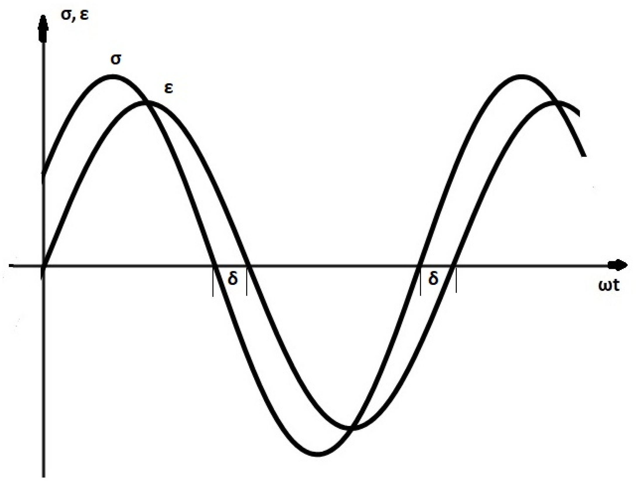
For small strains the mass density ρ can be considered as constant and it can therefore be put outside of the integral. The integral from t₁ to t₂ of $\dot{u}dt$ is equal to $u_2-u_1=0,$ since the internal energy u is a state function, and hence it has the same value at the end (time t₂) and the beginning (time t₁) of the cyclic process. The steady-state excitation, which we presented in Section 2, is a particular case of a cyclic process. Therefore, from the above Equation (5), whose left-hand side is equal to zero, it follows that the integral of the deformation power over a period is equal to the amount of heat produced, i.e., to the mechanical energy dissipated during this time. The integral of the deformation power is equal to the area of the stress versus the strain diagram in the one-dimensional case and to the summation of the areas of the conjugate stress-strain diagrams in multidimensional cases. It can be mentioned here that Tschoegl [9] arrives at the same result on the basis of the assumption that the kinetic energy can be neglected for a viscoelastic material. This assumption is unnecessary and is wrong in general.

The steady-state process, which we examined represents a “simple” case of loading-unloading of engineering materials and is frequently met in experimental works and in applications. If this is modeled by linear viscoelasticity the energy dissipated can be computed by the area of the stress-strain curve and by the summation of the areas of the conjugate stress-strain curves in multidimensional cases.

It should be noted that a thermodynamics framework, in addition to its other advantages, e.g., consistency between assumptions made and constitutive models, gives us the tools to identify the different mechanisms contributing to energy dissipation such as viscoelasticity and damage [4].

3.2. Calculation of Dissipated Energy by the Second Law of Thermodynamics

We will now compute the dissipated energy by using the second law of thermodynamics for comparison purposes with the results obtained by the first law and for completeness and moreover in order to address more general material descriptions (constitutive hypotheses) and loading conditions. In particular, dissipative materials which can be described by the use of internal variables are addressed. Internal variables in mechanics and constitutive modeling is a rich and vast subject, which has been very successful. Modern inelasticity, computational inelasticity, and damage mechanics models are based on internal variables.

There are many publications on this subject and we refer here to some of them, e.g., [1,2,10,11] for nonlinear finite viscoelasticity, [12,13,14,15] for a new concept in internal variables. Within the framework of internal variables, the linear and nonlinear theories of viscoelasticity for small as well as finite deformations have been successfully formulated and applied for material modeling. The same is true for the theories of elasto-plasticity, elasto-viscoplasticity, and damage mechanics. Material models that are developed within the framework of internal variables are usually amenable to efficient implementation into computational mechanics codes, such as finite elements. Important finite element frameworks, such as ABAQUS, ANSYS, and OPENSEES to name a few use the concept of internal variables. The second law of thermodynamics may be expressed by the Clausius-Duhem inequality, which has as a result the Kelvin inequality (dissipation inequality), see e.g., [1,16,17]. i.e.,

$$D\ge 0,$$

(6)

where D is the intrinsic dissipation given by

$$D={\displaystyle {\sum }_{\alpha }{p}_{\alpha }}{\dot{\xi }}_{\alpha }.$$

(7)

In Equation (7) $p_{\alpha }$ are the “thermodynamic forces” conjugate to the internal variables ξ_α, which constitute the internal variable vector ξ. The subscript α in the internal variables ξ denotes their number (α = 1…n). The “thermodynamic forces” $p_{\alpha }$ are given as

$$p_{\alpha }=-\rho {\displaystyle \frac{\partial \psi }{\partial {\xi }_{\alpha }}},$$

(8)

where ψ is the Helmholtz free-energy density per unit mass, see e.g., [1,13,16,17].

By employing the summation convention over the index α and by combining Equations (7) and (8) we have the following expression for the dissipation

$$D=-\rho {\displaystyle \frac{\partial \psi }{\partial {\xi }_{\alpha }}}{\dot{\xi }}_{\alpha }.$$

(9)

The decomposition of the strain tensor ε additively, in the case of small strains, into an elastic ε^e and an inelastic part ε^ι is equivalent to the decomposition of the free energy into elastic and inelastic components as follows [18]

$$\psi (\mathit{\epsilon },\theta ,\xi )={\psi }^e(\mathit{\epsilon }-{\mathit{\epsilon }}^i(\xi ),\theta )+{\psi }^i(\xi ,\theta ),$$

(10)

where θ is the absolute temperature.

As is well known the free energy density ψ serves as a potential for the (Cauchy) stress tensor σ, i.e.,

$$\mathit{\sigma }=\rho {\displaystyle \frac{\partial \psi }{\partial \mathit{\epsilon }}}$$

(11)

see e.g., [13].

Therefore, from Equations (10) and (11) we obtain the following useful expression for the stress tensor σ since ${\psi }^i$ is independent of ε,

$$\mathit{\sigma }=\rho {\displaystyle \frac{\partial {\psi }^e}{\partial {\mathit{\epsilon }}^e}}.$$

(12)

Because of Equations (10)–(12) and by using the relation ${\dot{\mathit{\epsilon }}}^i={\displaystyle \frac{\partial {\mathit{\epsilon }}^i(\xi )}{\partial {\xi }_{\alpha }}}{\dot{\xi }}_{\alpha }$ the dissipation now (Equation (9)) reads:

$$D=\mathit{\sigma }:{\dot{\mathit{\epsilon }}}^i-\rho {{\displaystyle \frac{\partial \psi }{\partial {\xi }_{\alpha }}}}^i{\dot{\xi }}_{\alpha }$$

(13)

where the term $\mathit{\sigma }:{\dot{\mathit{\epsilon }}}^i$ represents the rate of the inelastic work per unit volume. We will now consider a cyclic process from time t₁ to time t₂ and will compute the dissipation, through this cyclic process, by integrating D. We will proceed by first integrating the first term of D, in Equation (13).

We then obtain

$${\displaystyle {\int }_{t_1}^{t_2}\mathit{\sigma }:{\dot{\epsilon }}^i}dt={\displaystyle {\int }_{t_1}^{t_2}\mathit{\sigma }:\dot{\epsilon }dt}-{\displaystyle {\int }_{t_1}^{t_2}\mathit{\sigma }:{\dot{\epsilon }}^e}dt.$$

(14)

By using Equation (12) the second integral of the right-hand side is equal to ρ[Ψ^e(t₂) − Ψ^e(t₁)] and is zero for isothermal conditions. (Material density ρ has been taken out of the integral because of small strains.) This is because the elastic free energy is a function of ε^e and θ (see Equation (10)).

Since σ is a function of ε^e and θ, i.e., σ = σ(ε^e, θ) because of Equation (12), it holds that ε^e = ε^e(σ, θ) because of the inverse mapping theorem of advanced calculus. At times t₁ and t₂ the stress has the same values (cyclic process) and therefore the elastic strains also under isothermal conditions and subsequently the elastic free energy components Ψ^e(t₁) and Ψ^e(t₂).

Therefore, the dissipated energy in a cyclic process from t₁ to t₂ is

$$\begin{array}{l}{W}_d={\displaystyle {\int }_{t_1}^{t_2}Ddt}={\displaystyle {\int }_{t_1}^{t_2}\mathit{\sigma }:\dot{\epsilon }dt}-{\displaystyle {\int }_{t_1}^{t_2}\rho {\frac{\partial \psi }{\partial {\xi }_{\alpha }}}^i{\dot{\xi }}_{\alpha }dt.}\\ \end{array}$$

(15)

Strains ε and stresses σ attain the same values at the beginning and end of the cycle. If we assume that in such a cycle and for isothermal conditions the internal variable vector ξ also has the same values at the beginning and end of the cycle then the second integral of the Equation (15) becomes $\rho ({\psi }^i(t_2)-{\psi }^i(t_1))=0,$ since Ψⁱ = ψⁱ(ξ, θ).

Therefore,

$$W_d={\displaystyle {\int }_{t_1}^{t_2}Ddt}={\displaystyle {\int }_{t_1}^{t_2}\mathit{\sigma }:\dot{\epsilon }dt}.$$

(16)

Therefore, we arrived at the same result as before, i.e., the dissipated energy is given by the area of the stress-strain diagram—in the one-dimensional case—when a complete cycle is considered, as for example in steady-state dynamic excitations over one period.

It is noted that the derivations above were carried in a direct tensorial notation.

One may want to use indicial notation and obtain the same results.

Remarks

1. From Equation (16) it is clear that in a multi-dimensional case, the dissipated energy is equal to the sum of the areas of the conjugate stress-strain diagrams. To the best of our knowledge, this is a new result, which has not been reported elsewhere.

2. It is reasonable to assume that since ε(σ, θ, ξ) and σ attain the same values at the beginning and end of the cycle then in such a process and for isothermal conditions the internal variable vector ξ also has the same value at the beginning and end of the cycle. In this case, Equation (16) follows from (15) under isothermal conditions only.

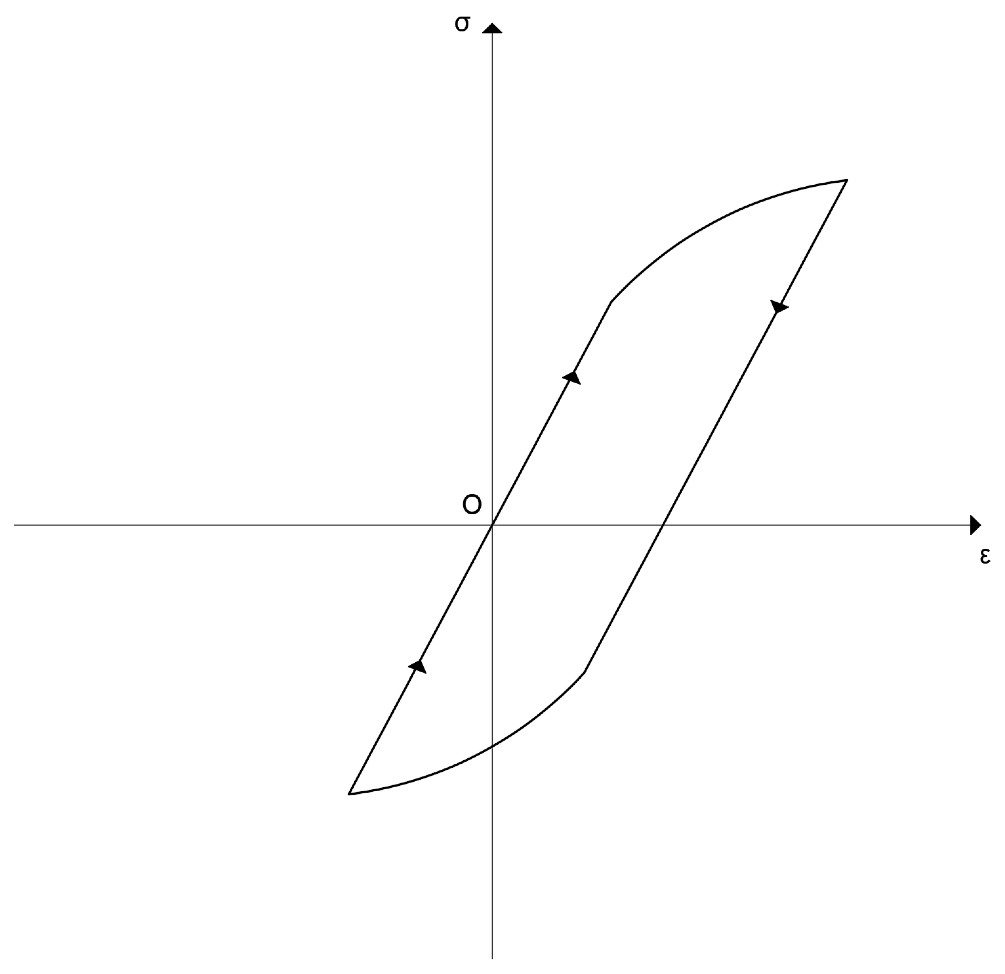
However, as pointed out by Lubliner [1] (page 64 and figure on this page) it is possible that a situation like the following arises in an inelastic material (see the following Figure 2, which is reproduced from Lubliner for the reader’s convenience). The loading starts from point O and returns to it. At the end of the cycle, the stress σ has returned to its initial value, i.e., zero, as well as the total strain ε. Nevertheless, the internal state of the material may be different from its initial state, which means that some of the internal variables introduced for the description of the material’s behavior and modeling have not returned to their initial values at the end of the cycle.

Therefore, in such a case Equation (16) does not hold and we must use Equation (15), in order to include the contribution of the internal variables, for the computation of the dissipated energy.

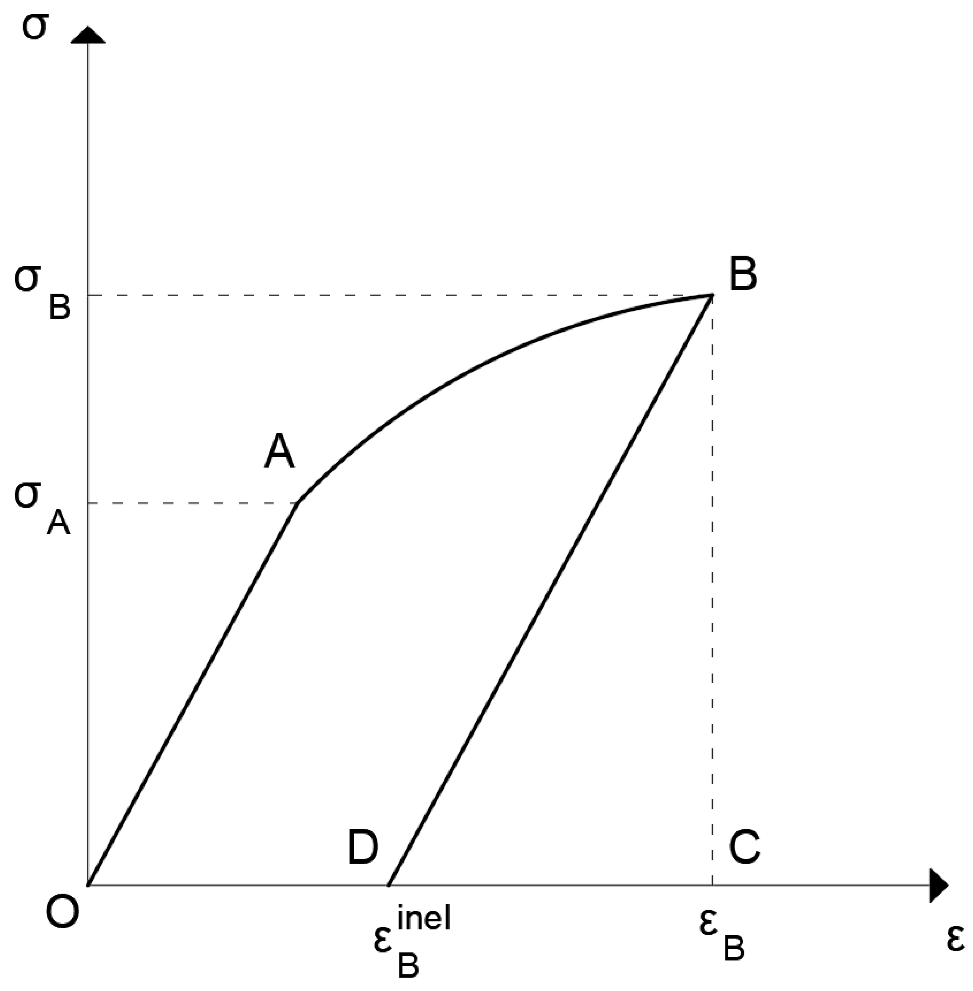
3a. In the following figure (Figure 3) the typical one-dimensional loading-unloading curve of an elastoplastic material is shown, with a single internal variable being the ${\epsilon }^{inel}$ (permanent strain). If we consider the loading path from O to A to B and then start unloading from point B to point D, i.e., until the stress becomes zero and the strain is equal to ${{\epsilon }_B}^{inel}$, then clearly in this path the stress returns to its initial value (zero) but neither the total strain ε, which is equal to ${{\epsilon }_B}^{inel}$ does nor the internal variable, which is equal to ${{\epsilon }_B}^{inel}$. It is noted that in the figure the segment DC represents the elastic strain (the recoverable strain) at point B. Therefore, in this case, even under isothermal conditions the area of the loop OABD does not represent the dissipated energy!

It is emphasized that in publications, including papers, theses, doctoral dissertations, and even books, this is a common mistake made by their authors designating this area as dissipated energy. See, e.g., the book [19] (Figure 3.18, p. 114).

3b. A similar mistake is found in cases of one cycle or of repeated cycles of loading- unloading. This error frequently appears again in publications, including papers, theses, doctoral dissertations, books, and even engineering codes. For example, in [20], p. 99, Figure 7.1, (see also Figure 7.7N, p. 115) it is stated that the dissipated energy per cycle is equal to the area of the loop. This is wrong according to our development. It should have been stated that this is valid for isothermal conditions and therefore Eurocode’s 8 assertion is an assumption. Moreover, it should have been reported if the internal variables of the model used in order to obtain Figure 7.1 are returning to their initial values in each cycle. The same remarks apply to many papers in structural engineering, see e.g., [21] among many others.

3c. Apart from structural engineering and structural mechanics, similar erroneous calculations are found in soil mechanics works. For example, such results are usually found in energy methods for the evaluation of soil liquefaction, where the area under a stress-strain curve is assumed to represent the dissipated energy, see e.g., [22,23] among others.

4. In case the internal variables do not return to their initial values in an isothermal loading process the dissipated energy is given, as we proved, by Equation (15), which is repeated below, i.e., as

$$W_d={\displaystyle {\int }_{t_1}^{t_2}\mathit{\sigma }:\dot{\epsilon }dt}-{\displaystyle {\int }_{t_1}^{t_2}\rho {\frac{\partial \psi }{\partial {\xi }_{\alpha }}}^i{\dot{\xi }}_{\alpha }dt}$$

(17)

Therefore, it is not given by just the sum of the areas of the conjugate stress-strain diagrams but it consists of two parts. Both parts should be taken into account for the correct computation of the dissipated energy. This result also underlines the importance of the choice of the internal variables, i.e., of the constitutive modeling.

A developer of a model knows the model’s internal variables and their evolution equations as well the form of the inelastic part of the free energy ψⁱ. Therefore, the model’s developer knows if the internal variables return to their initial values at the end of a cycle and in case the second part of Equation (17) is needed the modeler can compute it. If this is the case, the contribution of each term of Equation (17) to the dissipated energy W_d. is calculated,

5. It is worth mentioning that there are more general cases in inelastic constitutive modeling in which the material neighborhood has structure, and its geometry should be represented by a non—Euclidean metric g, called a material metric (or physical metric) [15]. Modeling by material metric is within the area of internal variables. Therefore, the results presented here regarding the dissipated energy are valid for these more general cases too, with the new internal variable g included in the relevant computations.

3.3. Dissipated Energy in Terms of Loss Tangent

We now use the results obtained in Section 3 and we return to Section 2 in order to calculate the dissipated energy per unit volume in a complete cycle and for a linear viscoelastic material.

For this purpose, by using Equations (1) and (2) in Equation (16) we obtain the following expression for the dissipated energy

$$W_d={\displaystyle \int \sigma d\epsilon ={\displaystyle {\int }_0^{2\pi /\omega }{\sigma }_0}}\sin (\omega t+\delta ){\epsilon }_0\omega \cos (\omega t)dt,$$

and by performing the integration over a period the above relation yields,

$$W_d={\sigma }_0{\epsilon }_0\pi \sin \delta .$$

(18)

Hence, the tangent of the phase angle δ, known as the loss tangent, is

$$\tan \delta ={\displaystyle \frac{W_d}{\pi {\sigma }_0{\epsilon }_0\cos \delta }}.$$

(19)

From this equation the direct relation of the loss tangent with the dissipated energy is clear, and therefore so is its significance in applications.

The strain attains its maximum value ε₀ at t = T/4 and the corresponding value of the stress is σ = σ₀cos δ. If W_s denotes the stored energy of a linear elastic material strained up to ε₀ with corresponding stress σ = σ₀cosδ, then W_s is

$$W_s=1/2{\sigma }_0{\epsilon }_0\cos \delta .$$

Hence,

$$\tan \delta ={\displaystyle \frac{W_d}{2\pi W_s}}.$$

(20)

Relation (20) is frequently used in applications.

4. Discussion and Conclusions

In this work, we related the frequently used term hysteresis to linear viscoelasticity and steady-state excitations, and we pointed out the misleading way this term is used for any inelastic constitutive law and without hysteresis being present.

By using the laws of thermodynamics, we computed the energy dissipated in a viscoelastic material, and more generally in an inelastic material modeled with the use of internal variables. Our results were derived in a multidimensional framework being indispensable for calculations in multiaxial stress and strain conditions. We identified the conditions under which the area of the σ-ε curve, or more generally in multiaxial cases the sum of the areas of the conjugate stress-strain diagrams, represents the dissipated energy. There is an abundance of papers in the literature calculating the “energy dissipated” by computing the area of a strain-stress curve, or an area of a curve of other conjugate quantities (i.e., cross-section resultant forces and generalized displacements), without any explanation or proof of why this is so.

We have not seen a work that calculates the dissipated energy and explains why an area measures the dissipated energy. Moreover, nowhere has been reported as to why in multiaxial cases the dissipated energy is computed as the sum of the areas of the conjugate stress-strain diagrams.

In addition, we showed why those calculations are erroneous unless specific conditions, which we identified, hold. In isothermal conditions the exact form of the dissipated energy is given by Equation (17) (or Equation (15)). Isothermal conditions can be attained in a laboratory environment, but it may be difficult otherwise. In case the internal variables do not return to their initial values in an isothermal loading process Equation (17) should be used.

Therefore, in this case, the area of a “stress-strain curve” is part of the energy dissipated as it was shown here; see Remark 4 in Section 3.2. In this case for the correct computation of the dissipated energy the second part of Equation (17) i.e., the term ${\displaystyle {\int }_{t_1}^{t_2}\rho {\frac{\partial \psi }{\partial {\xi }_{\alpha }}}^i{\dot{\xi }}_{\alpha }dt}$ must be included in the energy dissipated.

We note in passing that this is another example of the importance of internal variables in constitutive modeling.

If this part is not included the dissipated energy calculated is an approximation of its correct value.

It should be added that such approximate computations of the dissipated energy by an area are found in many domains of solid mechanics and material modeling and applications, e.g., in soils, metals, fatigue, shape-memory alloys, and so on.

In addition, there are many textbooks and even engineering codes that make the same mistake.

The calculations which we presented here are in the domain of small strains and rotations. It is interesting and important that our formulation be extended to the range of moderate and large strains. With respect to this remark, the following note is worth mentioning here: Apart from the fully finite deformation cases (i.e., large strains and large rotations) there are many cases in engineering applications and modeling with moderate or large rotations and small strains. These cases can be addressed correctly only within the framework of fully finite deformation theories. The extension of our approach to finite deformations will be pursued in a forthcoming publication.

Furthermore, the work presented here constitutes a solid and very useful application of thermodynamics to material and structural modeling and description.

It also provides an answer to criticisms that thermodynamics is a formalistic framework with little if any use in constitutive modeling.

References

1. Lubliner, J. Plasticity Theory; Macmillan Publishing Company: New York, NY, USA, 1990. [Google Scholar]
2. Lubliner, J.; Panoskaltsis, V.P. The Modified Kuhn Model of Linear Viscoelasticity. Int. J. Solids Struct. 1992, 29, 3099–3112. [Google Scholar] [CrossRef]
3. Mehta, P.K.; Monteiro, P.J.M. Concrete, Microstructure, Properties and Materials, 3rd ed.; McGraw-Hill: New York, NY, USA, 2006. [Google Scholar]
4. Panoskaltsis, V.P.; Bahuguna, S. Micro and Macromechanical Aspects of the Behavior of Concrete Materials with Special Emphasis on Energy Dissipation and on Cyclic Creep. J. Mech. Behav. Mater. 1996, 6, 119–134. [Google Scholar] [CrossRef]
5. Golden, J.M.; Graham, G.A.C. Boundary Value Problems in Linear Viscoelasticity; Springer: New York, NY, USA, 1988. [Google Scholar]
6. McCrum, N.G.; Buckley, C.P.; Bucknall, C.B. Principles of Polymer Engineering, 2nd ed.; Oxford University Press: Oxford, UK, 1997. [Google Scholar]
7. Green, A.E.; Naghdi, P.M. On Thermodynamics and the Nature of the Second Law. Proc. R. Soc. Lond. 1977, 357, 253–270. [Google Scholar]
8. Morro, A.; Giorgi, C. Techniques for the Thermodynamic Consistency of Constitutive Equations. Thermo 2023, 3, 260–276. [Google Scholar] [CrossRef]
9. Tschoegl, N.W. The Phenomenological Theory of Viscoelastic Behavior: An Introduction; Springer: New York, NY, USA, 1989. [Google Scholar]
10. Dafalias, Y.F.; Popov, E.P. Plastic Internal Variables Formalism of Cyclic Plasticity. J. Appl. Mech. 1976, 43, 645–651. [Google Scholar] [CrossRef]
11. Simo, J.C. On a Fully Three-dimensional Finite-Strain Viscoelastic-Damage Model: Formulation and Computational Aspects. Comput. Methods Appl. Mech. Eng. 1987, 60, 153–173. [Google Scholar] [CrossRef]
12. Maugin, G.A. The saga of internal variables of state in continuum thermo-mechanics (1893–2013). Mech. Res. Commun. 2015, 69, 79–86. [Google Scholar] [CrossRef]
13. Ottosen, N.S.; Ristinmaa, M. The Mechanics of Constitutive Modeling, 1st ed.; Elsevier: New York, NY, USA, 2005. [Google Scholar]
14. Horstemeyer, M.F.; Bamman, D.F. Historical review of internal state variables for inelasticity. Int. J. Plasticity 2010, 26, 1310–1334. [Google Scholar] [CrossRef]
15. Panoskaltsis, V.P.; Soldatos, D.; Triantafyllou, S.P. The Concept of Physical Metric in Rate–Independent Generalized Plasticity. Acta Mech. 2011, 221, 49–64. [Google Scholar] [CrossRef]
16. Besson, J.; Cailletaud, G.; Chaboche, J.-L.; Forest, S.; Bletry, M. Non-Linear Mechanics of Materials; Springer: New York, NY, USA, 2010. [Google Scholar]
17. Lemaitre, J.; Chaboche, J.-L. Mechanics of Solid Materials; Cambridge University Press: Cambridge, UK, 1990. [Google Scholar]
18. Lubliner, J. On the Thermodynamic Foundations of Nonlinear Solid Mechanics. Int. J. Nonlinear Mech. 1972, 7, 237–254. [Google Scholar] [CrossRef]
19. Popov, E.P. Engineering Mechanics of Solids, 2nd ed.; Prentice Hall: Hoboken, NJ, USA, 1999. [Google Scholar]
20. EN 1998-2:2005+A2; Design of Structures for Earthquake Resistance—Part 2: Bridges; Eurocode 8, English Version. European Committee for Standardization: Brussels, Belgium, 2011.
21. Golias, E.; Vougioukas, E.A.; Wittemannc, K.; Kalogeropoulos, G.I.; Karayannis, C. Cyclic Response of RC Beam-Column Joints Strengthened with Transverse Steel Bars and with C-FRP Diagonal Ties. Acta Polytech. 2022, 62, 274–282. [Google Scholar] [CrossRef]
22. Figueroa, J.L.; Saada, A.S.; Liang, L. Effect of the Grain Size on the Energy per Unit Volume at the Onset of Liquefaction. In Proceedings of the Third International Conferences on Recent Advances in Geotechnical Earthquake Engineering and Soil Dynamics, St. Louis, MO, USA, 2–7 April 1995; Volume 1, pp. 197–202. [Google Scholar]
23. Alavi, A.H.; Gandomi, A.H. Energy-based numerical models for assessment of soil liquefaction. Geosci. Front. 2012, 3, 541–555. [Google Scholar] [CrossRef]
Figure 1. Oscillatory stress and strain in linear viscoelasticity showing phase angle δ (hysteresis angle).
Thermo 05 00020 g001
Figure 2. Closed stress-strain cycle for an inelastic material. Stress and strain return to zero at the end of the cycle, point O but the material’s internal state may have changed (from [1]).
Thermo 05 00020 g002
Figure 3. Typical stress-strain curve of an inelastic material. Loading-unloading.
Thermo 05 00020 g003
Disclaimer/Publisher’s Note: The statements, opinions and data contained in all publications are solely those of the individual author(s) and contributor(s) and not of MDPI and/or the editor(s). MDPI and/or the editor(s) disclaim responsibility for any injury to people or property resulting from any ideas, methods, instructions or products referred to in the content.