Abstract
Thermal modelling of additive manufacturing is a key method for furthering the quality of the components produced, as it allows for analysis that is not possible via experimental methods due to the difficulties involved with in situ monitoring. The thermal gradients present during the additive manufacturing process have a large impact on the formation of defects, such as porosity, residual stress, and cracking. The thermal gradients also have a large impact on material properties by controlling the microstructure formed. Thermal modelling methods are often based on numerical solutions of the heat conduction equation. Whilst numerical methods can be more accurate, they are often very slow because of the fine mesh requirements to capture high thermal gradients and iterative solvers to approximate the real-world solution to the required thermal field equations. An analytical model was developed to provide a fast solution to the problem. The analytical model used in this research was based on the Rosenthal equation and was analysed under a range of process parameters. A temperature-dependent Rosenthal model was also created with the aim of improving the results. The analytical model was then compared with a finite element numerical model to act as verification for the results. The analytical model accurately predicted the meltpool width over a range of process conditions. The analytical model underestimated the meltpool length compared to the numerical model, especially at high velocities. When using the standard Rosenthal model, the use of room-temperature or high-temperature thermal conductivities underestimated or overestimated the cooling rates from the meltpool, respectively. A temperature-dependent Rosenthal model was shown to produce more accurate cooling rates compared to the original Rosenthal equation.
1. Introduction
Additive manufacturing (AM) has been a rapidly growing method of manufacturing that offers numerous advantages over conventional methods. Metal additive manufacturing refers to the production of a component via the deposition and selective melting of subsequent metal powder layers via an external heat source. There are multiple different types of additive manufacturing, with the main distinctions being the type of heat source used and the powder deposition method. Laser powder bed fabrication (L-PBF) is a powder bed fusion AM technique, which involves the use of a high-energy-density laser to selectively melt and consolidate subsequent metal powder layers that are 100 μm thick in the powder bed [1].
AM allows for the relatively fast creation of near-netshape complex components, which would not be achievable by conventional manufacturing methods [2]. The increased design freedom allows for more complex designs, which allow for an increase in the operating efficiency of the component due to lighter and stronger designs. The AM process allows for the manufacture of novel component designs, which would be more difficult with traditional manufacturing methods. Also, the AM process does not require the same level of post-processing as conventional methods, which means that the creation of the component is faster and there is less waste of material, whilst also simplifying the process. An example of this is in the aerospace industry—especially high-temperature jet engine components—where the increased freedom of design allows for significant engineered design benefits with lighter components and the creation of rapid prototypes, allowing for a faster time to market.
One high-temperature alloy that is extensively used in additive manufacturing is Inconel-718 [3]. Inconel-718 is an austenitic Ni-Fe-Cr nickel-based superalloy, composed of a γ matrix phase (Ni-Fe-Cr) and a precipitate γ′ phase (Ni3(Al,Ti,Nb)). Nickel superalloys have excellent high-temperature creep and fatigue properties, paired with good high-temperature corrosion resistance, which makes these alloys ideal for high-temperature and high-stress applications, such as turbine blades in airplane engines [4]. The exceptional high-temperature properties allow for higher engine temperatures, which help to increase the performance of the engine. In comparison to other nickel superalloys, Inconel 718 has a much higher weldability, which makes it much more suitable for additive manufacturing. The increase in weldability of the alloy reduces the chances of weld cracking due to the intense heating rates present during additive manufacturing. The weldability of nickel superalloys is a function of the Al and Ti content.
Additive manufacturing is a complex process in which small changes to the processing parameters can lead to the formation of defects. During the additive manufacturing process, high temperature gradients are caused by fast heating rates and relatively slow thermal conduction throughout the metal. The steep thermal gradients lead to uneven thermal expansion throughout the metal, resulting in tensile and compressive stresses in the component [5,6]. These residual stresses lower the strength of the component and, in some cases, can lead to the formation of cracks. The magnitude of residual stress can be controlled by the material composition and by the fine control of the process parameters to try to reduce the temperature gradients.
In additive manufacturing, the shape of the thermal fields, and thus, the quality of the produced component, is largely controlled by the material choice and the critical process parameters, including laser power, scanning speed, and bed temperature. However, as discussed by Everton et al. [7], in situ monitoring of the AM process is difficult because of the short time scale and extremely high temperature gradients. Modelling is a possible alternative method to understand the thermal fields, as it enables analysis of both the thermal and mechanical conditions within the component throughout the process [8,9]. Due to the high level of complexity in the different interactions happening throughout additive manufacturing, different length–scale models tend to be implemented, depending upon the desired process predictions. Thus, the various important aspects of AM have been broken down into separate models: residual stresses using finite elements (FEs) [5], whereby authors predict stress evolution throughout a build; microstructural development predictions using cellular automata [10]; and modelling of complex powder behaviour using particle dynamics [11].
Throughout the literature on additive manufacturing, different types of models have been studied, with the main areas of research focusing upon either analytical or numerical modelling [9]. Analytical modelling is a mathematical modelling method in which simple equations based on physical laws and physical processes are used. The use of simple fundamental equations allows analytical methods to be much faster to compute and to give an intuitive understanding of the process. For purely thermal field solutions within linear moving heat source processes, the Rosenthal equation offers a concise solution for engineers to apply an analytical method [12,13].
Promoppatum et al. [14] utilised an analytical framework to predict the meltpool dimensions of laser powder bed Inconel 718 with excellent accuracy from the baseline Rosenthal equation. Because analytical models are much faster, they can be integrated into other modelling methods investigating different areas of the process, such as microstructure evolution [15].
Numerical models for thermal fields utilise mathematical solutions to find approximate solutions to the physical processes in question [16]. For all types of modelling methods, certain assumptions are required to reduce the complexity of a model. Numerical models normally have the ability to model more complex physical phenomena and thus can produce more accurate results. However, these methods require more computational power and time in comparison to analytical methods because of the more complex equation sets that are to be solved.
In the literature, there have been multiple attempts to improve the accuracy of AM analytical models of additive processes, such as laser powder bed fabrication (L-PBF) [17,18] and direct-laser deposition (DLD) [19], by reducing the dependence upon less accurate common assumptions, including (i) temperature independent material thermophysical properties, (ii) steady-state temperature distributions, (iii) a point heat source, and (iv) ignoring heat transfer effects of convection and radiation [17].
Mirkoohi et al. [20] produced an analytical model based on an adapted Rosenthal equation, aiming to reduce the assumptions in previous models by taking into account factors such as latent heat, thermal dependent properties, and effects of build layers. The model produced was compared to both experimental results and numerical modelling results for verification. The model was found to be accurate to 7.6% when compared to the experiment. The model predicted higher temperatures than observed experimentally, which was attributed to the thermocouple tip location during the experiment. However, the high peak temperature could also be caused by ignoring the effects of surface heat losses from convection and radiation. In addition, Steuben et al. [21] developed so-called enriched analytical solutions for additive manufacturing, including temperature-dependent thermophysical properties, which were capable of matching FE simulations.
Within the similar field of laser welding, Hekmatjou et al. [22] developed a Rosenthal analytical model for an aluminium alloy and compared the results to FE predictions. They found that the Rosenthal equation overestimates the meltpool dimensions. This was attributed to the assumptions made in the analytical Rosenthal equation in terms of neglecting heat losses through the substrate.
A closed-form analytical procedure was developed by Moda et al. [23] for the Rosenthal equation representing a moving heat source in a semi-infinite solid. The work presented a dimensionless comparison of additive manufacturing heating to traditional welding. The model was interrogated and extended to predict the lack-of-fusion defects in AM and void surface fraction, highlighting the adaptability that analytical solutions offer.
Correa-Gomez et al. [24] implemented a concept known as the ‘thermal dose’, namely, the thermal gradient multiplied by an applied time, to improve predictions of meltpool geometry. They utilised the linear energy density of a beam heat source to allow the Rosenthal equation to be solved for combinations of beam speed and power, followed by a computation of the thermal dose term, to define a near-semicircular meltpool shape in the experimental weld. The iterative nature of the process allows for higher precision within the analytical framework developed.
Ning et al. [25] proposed an analytical model that aims to solve the issues of neglecting heat loss mechanisms to the environment by correctly modelling boundary conditions. In previous work, correct boundary conditions were modelled exclusively by numerical methods. Using this model, the researchers found a good agreement with experimental measures in different areas of the substrate, which illustrated the accuracy of applied boundary conditions.
When thermal models target high integrity and fidelity over computational efficiencies, computational fluid dynamics (CFD) methods remain the most accurate, owing to their treatment of the molten region within a molten pool as a fluid. Hozoorbakhsh et al. [26] developed CFD capabilities to predict accurate pool formations for variation in additive manufacturing, with the beam speed and power entered as input parameters for a type of stainless steel. Their findings showed that the pool shape became more elliptical at higher travel speeds and powers. In contrast, Ai et al. [27] implemented a volume of fluid approach to predict the highly complex keyhole vapour phase within high-energy-density laser beam welds, for both a continuous and an oscillating heat source. The resulting keyhole geometry demonstrated fluctuations at the same period as the oscillating heat source, highlighting the highly transient nature of keyhole formation. Whilst CFD and volume of fluid approaches offer high accuracy, this comes at the additional computational costs of much longer run times.
As such, there is increasing industrial and academic interest in developing analytical modelling frameworks, with rapid computation times, to present a more informed and flexible toolkit for additive manufacturing (AM) shop-floor technicians, additive manufacture engineers, and scientists, which will help solve the thermal field for common and novel additive processes with considerable fidelity and accuracy. The present work explores the accuracy of a Rosenthal analytical model for AM thermal fields, in comparison to more detailed but slower finite element models, over a range of process parameters. This work studies how the accuracy of a simple analytical model can be improved whilst maintaining its fast calculation speed. Finally, the development of a fast and accurate method for solving the thermal field solution is important to allow for rapid process developments to improve AM procedures when the thermal field is the overriding factor.
2. Methods
2.1. Material and Processing Conditions
To create an accurate model, the required material thermophysical properties across the relevant temperature range were needed. In order to calculate the material properties, the commercial material properties software JMatPro (version 8.1), using the nickel superalloy module [28] by Sente software developers, was used to create temperature-dependent tables of the required properties, including density, thermal conductivity, and specific heat capacity. All calculations were performed for the nominal chemical composition of the Ni-based superalloy Inconel-718, as given in Table 1.

Table 1.
Chemical composition of the nickel (NiFeCr) superalloy Inconel 718 [29].
Analysis of published work on the AM of IN718 has shown that typical process parameters fall into a characteristic process window. The process conditions used during the systematic variation in weld speed, beam power, and bed temperature are shown in Table 2, which were chosen in accordance with other work in the open literature [2,30,31]. A finite element numerical model was used as a comparison to the analytical model to verify the generated results.
Table 2.
Matrix of testing conditions for the laser powder bed (L-PBF) deposition.
In both the FE model and the analytical model, a continuous material representation was used instead of a discrete powder method. Thus, the model assumes that the material is ‘solid’ and does not take into account the powder layer present on the surface. However, the assigned ‘solid’ object is given the relative thermal properties of a layer of powder to best match the real additive manufacturing environment. It is understood that the powder layer would have the effect of thermally insulating the meltpool because of the lower effective thermal conductivity of the powder on the top level of the material; however, this has not been replicated within either the analytical model or the FE model.
For the FE model, a temperature-dependent tabular dataset was used. For the analytical model, the values assigned are presented in Table 3. This effect would slightly change the shape of the meltpool; however, the relationships present between the thermal fields and the parameters would still be the same. The effect of fluid flow in the melt was not considered in the models, as this would have also added complexity that is outside the scope of this work.
Table 3.
Assumed thermophysical properties used in the analytical model.
2.2. Analytical Model
The Rosenthal equation, as shown in Equation (1), was used in this work to model the thermal field created by a steadily moving heat source [32]. Initially developed for traditional welding methods, this model has been adopted for use in additive manufacturing because of the similarities between the two processes. The Rosenthal equation was coded into the commercial programming software Matlab (version R2017b) [33]. A two-dimensional Cartesian grid representing the top surface of the material was created, and the Rosenthal equation was used to generate values for the temperature at each point of the grid for a moving heat source along the x-axis. This equation is presented in Equation (1), where T0 is the initial temperature, in K; λ is the absorptivity; P is the beam power, in W; k is the thermal conductivity, in W/m∙K; r is the distance from the heat source, in m; V is the beam scanning velocity, in m/s; α is the thermal diffusivity, in K−1; and , to update the beam location. It is interesting to note that the thermal diffusivity k is the only bulk material property in the model.
To allow the Rosenthal model to work, we made a series of simplifying assumptions:
- (i)
- The Rosenthal model assumes a point source of heat, whereas the energy supplied from the laser beam will follow a Gaussian distribution. This point source modelling framework loses the ability to diffuse energy spatially, which is less problematic at slower speeds but leads to larger errors at high travel speeds. As the pool becomes more elliptical, with the tail getting longer, the residual effects of the heat in the tail get more erroneous.
- (ii)
- The model assumes a steady-state condition, which happens when the thermal fields have stabilised relative to the moving heat source.
- (iii)
- Heat losses via conduction are the only heat transfer mechanism considered, which means heat losses to the environment through surface convection and radiation are not considered. Although the process occurs very rapidly, and the molten pool is very small in comparison to the solid body, which would hopefully minimise the unaccounted for cooling in the Rosenthal equation, this could lead to the overestimation of the actual cooling rate. This could cause the cooling curves in a Rosenthal model to vary from those predicted by FE modelling, which does account for convective and radiative heat loss.
- (iv)
- The standard Rosenthal model does not take into account the temperature-dependent nature of the material’s thermophysical properties.
Thus, when using the Rosenthal equation, the modeller must make a choice whether to use the material properties—such as thermal conductivity and specific heat capacity—using data relevant to the solidus temperature or data relevant at lower temperatures. The effect of this choice on the results of the simulation is studied in the present work.
A temperature-dependent version of the Rosenthal equation was developed based on a very simple and efficient numerical scheme. This approach used temperature-dependent thermal conductivity and worked in a way similar to the model created by Mirkoohi et al. [20]. A standard Rosenthal model was used to predict the temperature at each point on the surface of the material. The temperature at each point was then used to calculate the corresponding thermal conductivity from tabulated temperature-dependent data, using a linear interpolation function to calculate conductivity at intermediate temperatures. The equations used for conductivity were fitted, as given in Table 4, and were based on the tabulated data generated in JMatPro (v8.1) [28]. This created a continuous function of thermal conductivities corresponding to the temperature field around the moving heat source. The Rosenthal equation was then used to recalculate the temperature field using the new local values for thermal conductivity.
Table 4.
Thermal conductivity linear functions for the temperature-dependent Rosenthal equation for Inconel 718.
2.3. Numerical Model
Numerical finite element (FE) modelling was used for baseline comparison with the analytical Rosenthal model. Numerical methods, such as the FE method, use mathematical solutions to find approximate solutions to physical processes in question. FE modelling has the advantage of requiring fewer assumptions in comparison to analytical methods. FE models take into account physical effects, such as temperature-dependent properties, heat losses via surface radiation and conduction, and Gaussian heat source distributions. Because of the ability to model more complex interactions, numerical modelling methods can produce more accurate results and, therefore, provide a comparison for the Rosenthal model. However, this causes the associated computational time to be much greater.
A finite element (FE) model of the laser beam interaction with the powder bed was created (Figure 1) and computed using a commercial software package developed by ESI, called Sysweld (version 2015), and associated meshing and pre-processing tools in Visual Environment [34]. Because of software limitations, the dimensions were entered as a factor of 10 larger than intended, with material properties recalculated accordingly, to produce a working ‘0.1 mm , s , kg’ unit system. The simulated plate represented a 3 mm wide by 0.5 mm deep by 10 mm long section of a powder bed welding path. The beam commenced and finished 3 mm away from the edges in the travel direction, yielding a short 4 mm weld stripe. The plate was wide enough to ensure that there was no interaction of the heat at either the edges or the base of the plate to minimise any error in the simulated meltpool.
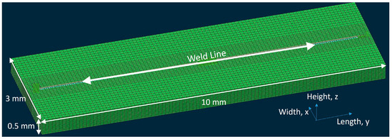
Figure 1.
An image from the Sysweld User Interface illustrating the modelling framework.
The graded mesh used in the FE calculations had an element size of 0.1 mm in the direction of the heat source travel and 0.05 mm in the perpendicular direction. A mesh sensitivity study was performed for modelling accuracy. A time-step of approximately 10−4 s was utilised, which was fine enough to allow the centre of the heat source to be present at least once in every element as it traversed along the weld path. These numerical modelling rules ensured that the FE modelling numerical parameters did not overly influence the result. As such, the FE solution was understood to be a fair comparison for the analytical solution. However, the FE model was still prone to some uncertainties, largely concerning the assumed heat source description and the discretisation of the object.
The FE model employed the standard double ellipsoidal Goldak function to describe the heat source. The double ellipsoid function is given in Equation (2), where are the local coordinates of the ellipsoidal model; η is the efficiency; Q is the beam power; can be either , i.e., the front semi axis, or , i.e., the rear semi axis; b and c are perpendicular and vertical semi-axes; and is either or , representing the heat portions of the heat flux in the front and rear quadrants, respectively, where .
Three-dimensional conical heat source descriptions are alternative heat source numerical models and are commonly used for electron beam processing [35]. Whilst the ellipsoid model is more commonly used for arc-type welding operations, developments in the literature have shown that for narrow-groove and keyhole weld pool geometries [36], or for a laser micro-welding process [37], some success is gained using this approach. As such, the ellipsoid model was selected within this work.
Thermal boundary conditions were implemented such that the powder bed had an initial temperature of either 20, 150, or 300 °C (293, 423, or 573 K), and the atmospheric air temperature was 20 °C, with convection set to 20 W/m2∙K. A mesh sensitivity study was conducted to establish the optimal meshing conditions that did not influence the FE predictions. A small difference between the lengths predicted with varying mesh sizes was noted, as shown in Figure 2, but it was considered negligible. The decrease in the element size across the width of the model had no effect on the produced widths of the weld pool.
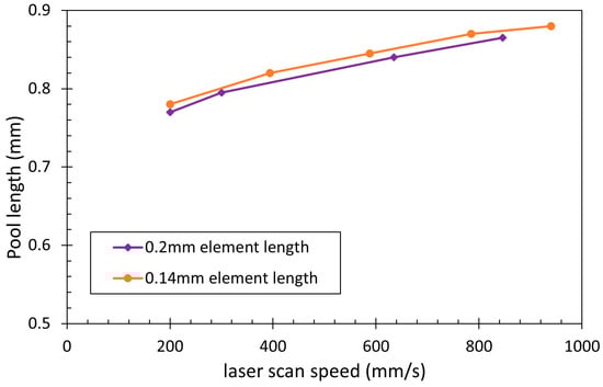
Figure 2.
Results of the mesh sensitivity study conducted to show the relative insensitivity of the predictions to numerical parameters.
3. Results
3.1. Standard Rosenthal Equation Sensitivity to Thermal Conductivity
In the finite element model created, the properties, such as thermal conductivity, are modelled as a temperature-dependent tabular dataset; see Figure 3. However, the standard analytical model uses constant thermal conductivity, which can have a large impact on the results generated. Inconel shows a large change in thermal conductivity over the relevant temperature range, increasing with temperature. At high temperatures, the thermal conductivity (28.2 Wm−1K−1) is over double the thermal conductivity at room temperature (11 Wm−1K−1). The low-temperature thermal conductivity simulations predict slower cooling rates than those that are realistic at high temperatures, i.e., at or near the meltpool; however, further away from the weld pool, they are more accurate. In the literature, there are multiple sources that use room-temperature thermal conductivities, which drastically underestimate the thermal conductivity.
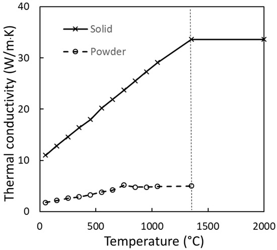
Figure 3.
Thermal conductivity of powder and solid Inconel 718 as a function of temperature.
In order to identify the value of thermal conductivity that is the most accurate to use in the Rosenthal equation, the two models, representing high and low thermal conductivity, respectively, were compared with the numerical model results. These results can be seen in Figure 4.
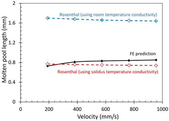
Figure 4.
Comparison of the meltpool length versus the scanning velocity for the numerical FE model and the analytic models using low and high thermal conductivity values.
The room-temperature Rosenthal equation results in a much longer meltpool in comparison to the numerical model. This is potentially caused by simplifications made by the analytical model to allow for the computation, including the point-source nature of the Rosenthal method and the lack of inclusion of convective and radiative heat loss terms, which physically must be present within the region of molten metal, albeit over an incredibly short temporal period. It could also be explained by the selection of the double-ellipsoid heat source description in the FE model over the 3D conical description. The high-temperature thermal conductivity Rosenthal equation results in a much more accurate value of the meltpool length in comparison to the FE model. The results show that the two different values for thermal conductivity used fall on either side of the FE results, which shows an overestimation and underestimation of the real physical phenomena.
From the results of the analytical model, it is seen that the temperature-dependent variation in thermal conductivity has a large effect on the predicted meltpool geometry. Both the high-temperature thermal conductivity and the room-temperature thermal conductivity models make the assumption that the thermal conductivities are constant throughout the material, albeit using different values. In reality, the thermal conductivity will be high in the area surrounding the meltpool and will be low in areas away from the meltpool.
3.2. Effects of the Processing Parameters on the Weld Pool Dimensions
To examine the effects of the laser beam power on the meltpool geometry, both the FE and Rosenthal models were simulated over a range of powers, i.e., 150 W to 350 W, at a constant velocity of 600 mm/s. It can be seen in Figure 5 that the increase in the beam power results in a sharp constant increase in the meltpool length and a gradual increase in the width in both models.
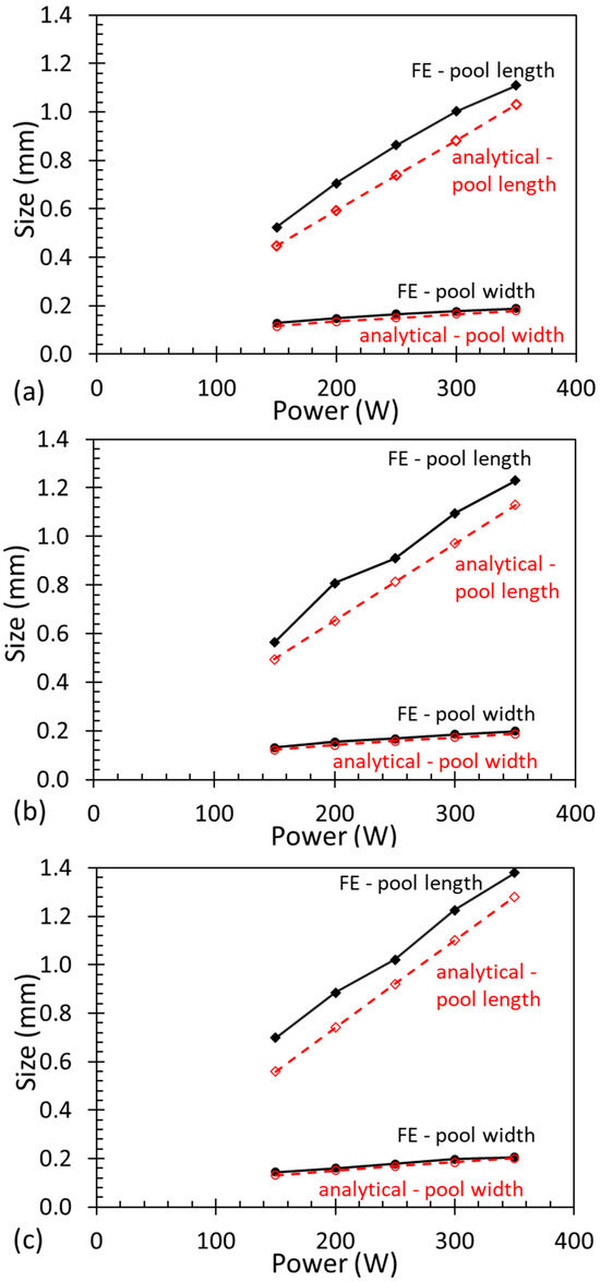
Figure 5.
Predicted meltpool geometry for beam powers of 150–350 W, at a fixed travel velocity of 600 mm/s and bed temperatures of (a) 293 K, (b) 423 K, and (c) 573 K.
The meltpool widths predicted by the Rosenthal equation are very similar to those of the numerical model. The length of the meltpool calculated by the Rosenthal equation slightly underestimates the length of the meltpool by a roughly constant amount. The effect of an increase in power is the same at all three bed temperatures.
Within an additive manufacturing operation, the scanning speed of the laser can have a significant impact on the thermal fields and the resultant geometry of the meltpool. Both the numerical and the analytical models were tested over a range of scanning speeds from 200 mm/s to 940 mm/s at 250 W. The results can be seen in Figure 6. Both the numerical and analytical models have similar results for the meltpool width over the range of velocities, showing a gradual decrease in the meltpool width with an increase in velocity.
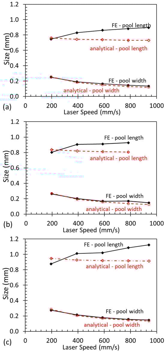
Figure 6.
Predicted meltpool geometry for travel speeds of 200–940 mm/s at a fixed beam power of 250 W and bed temperatures of (a) 293 K, (b) 423 K, and (c) 573 K.
3.3. Effects of the Bed Temperature on Thermal Cycles
The effect of the preheat temperature on the Rosenthal equation can be understood using the equation. As the bed temperature (T0) is a parameter added to the rest of the Rosenthal equation, the bed temperature will not have an effect on the heating and cooling rates found in the model and will just shift the heat and cooling curves upward. Figure 7 shows the heating and cooling rates of a point on the edge of the meltpool. The original Rosenthal equation predicts cooling gradients that are much higher than the numerical model predicts. This is likely because the Rosenthal equation cannot consider radiative and convective losses from the small molten pool and only calculates conductive losses through the bulk of the solid. This overestimation of the cooling gradients is present at all temperatures; however, the Rosenthal equation is more accurate than the numerical model at higher bed temperatures. Whilst out-of-scope for a thermal modelling methodology such as that developed in this work, the implications for the better fitting at higher bed temperatures are reassuring. Industrially, increasing the bed temperature is often performed to reduce thermal mismatch between the hot part and the cool substrate bed. This thermal mismatch can lead to higher residual stress formation at the base of the deposited build, which, in turn, leads to warping of the build or to cracking of the build [38].
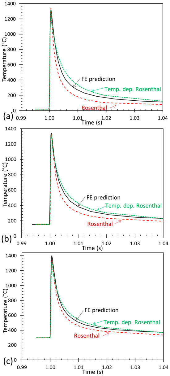
Figure 7.
Predicted thermal cycles for the numerical FE and Rosenthal models at bed temperatures of (a) 293 K, (b) 423 K, and (c) 573 K.
The temperature-dependent Rosenthal equation has a much better agreement with the numerical FE model, especially at higher bed temperatures. Initially, the temperature-dependent Rosenthal equation starts with an overprediction of the cooling rates and then later underestimates the cooling rates. In the temperature-dependent Rosenthal equation, there are some unrealistic sharp corners in the temperature gradients, which are caused by the method of calculating the thermal conductivity from linear segments.
4. Discussion
In the standard Rosenthal model, when using room-temperature properties, the thermal conductivity of the areas surrounding the meltpool size will be drastically underestimated, whilst it will be correct for areas far away from the meltpool. This assumption will have the effect of slowing the heat transfer away from the heat source. The slower diffusion of heat into the bulk of the material results in an increase in the length and width of the meltpool as it takes longer for the heat to dissipate. This is why the predicted meltpool size is much larger than that of the numerical FE model. Again, the potential errors within the FE model must be highlighted; the use of the double-ellipsoid heat source description in favour of the 3D conical description may add further sources of errors when comparing the results. It may be of interest to consider the conical heat source description in the future to compare to the predictions from standard and temperature-dependent Rosenthal approaches, as the conical heat source is a more traditionally used model for high-energy-density beams.
In contrast, when the standard Rosenthal equation uses the high-temperature thermal conductivity value, the meltpool will have an accurate thermal conductivity, whilst regions further away from the meltpool will have a large overestimation of the thermal conductivity. This inaccuracy in the thermal field causes a slightly faster conduction of heat away from the meltpool, which results in smaller predictions (15% smaller for P = 250 W and V = 600 mm/s) in the size of the meltpool.
Once the laser has reached a steady-state condition, the majority of the surrounding material will be at elevated temperatures, with thermal conductivities closer to matching the high-temperature thermal conductivities. When using the Rosenthal equation, the best thermal conductivity to use depends on the focus of the model. For areas far away from the meltpool, it is best to use room-temperature thermal conductivities, whilst for areas closer to the meltpool, high-temperature thermal conductivities are best.
As the power of the laser is increased, the energy input into the material increases. The results show that with the increase in power, there is a large increase in the meltpool length and a small increase in the meltpool width. The increase in dimensions is caused by the higher energy input, resulting in increased temperatures. The large increase in the meltpool length is due to the much higher temperatures reached, which takes longer for the heat to dissipate, resulting in a longer meltpool. This is known as the ‘meltpool lifetime’.
Both the analytical and numerical models show similar results for the predicted meltpool width with an increase in velocity. The models show a gradual decrease in width with an increase in velocity. As the scanning speed increases, the energy input decreases per unit length, which results in a decrease in the width of the meltpool.
Whilst the two models predict similar values for the length of the meltpool at low speeds, the models differ in the prediction of the relationship between increasing scanning speed and meltpool length. The numerical model predicts that as the velocity increases, the meltpool length will gradually increase. The analytical model predicts that over an increase in velocity, the meltpool length will gradually decrease. The findings in the literature support the results found in the numerical results [39].
The differences between the models are likely caused by the different assumptions each model makes. To study the effect that temperature-dependent properties have on the predictions, a numerical FE model was run with constant thermal properties. The results of this FE model showed a decrease in values of the pool length, but the values still increased with an increase in velocity, which shows that the difference was not caused by the temperature dependence of the material properties. The assumption of the point heat source in the Rosenthal equation should not affect the length of the meltpool as it is a sufficient distance away from the heat source. The Rosenthal model ignores the effects of radiative and convective losses from the surface, which could cause the results shown. A potential reason for the difference in velocity could be that as the velocity of the laser increases, the energy input per unit length (J/mm) decreases; this would have the effect of reducing the length of the meltpool. However, as the laser speed increases, the effect of heat losses to the environment for a point relative to the location of the heat source decreases because the time difference between the two points decreases, which has the effect of lengthening the meltpool.
The cooling rates during additive manufacturing have a larger effect on mechanical fields, such as residual stresses and microstructural development. Therefore, it is important for a model to accurately predict the thermal gradients that the model will experience. Numerical FE models can accurately predict the thermal gradients because they consider complex interactions that analytical modelling cannot. The results show the differences in the predicted thermal gradients between the Rosenthal equation and the numerical model for a point on the edge of the meltpool.
The original Rosenthal equation predicts the cooling rates to be much faster than the numerical model. This effect is caused by the assumption of non-temperature-dependent thermal properties. The model assumes high-temperature thermal conductivity, which is accurate for the area around the meltpool but is incorrect for the rest of the model. The increased thermal conductivity results in faster heat dissipation away from the meltpool, leading to faster cooling rates. The impact of the assumption decreases as the bed temperature increases, as this has the effect of raising the average thermal conductivity of the material.
The temperature-dependent Rosenthal equation attempts to solve the issues found in the standard Rosenthal equation by accounting for the change in thermal conductivity as the material cools down. Initially, the model predicts a faster cooling rate, but then, it changes to predicting lower cooling rates when compared to the numerical model. The initial overprediction of the cooling rate is caused by the same assumption as in the original Rosenthal model. The latter, slower cooling rate is caused by the thermal conductivity dropping as the temperature decreases. The underestimation is caused by the neglect of heat loss mechanisms, such as surface convection and radiative heat losses. For the model to solve this, correct thermal boundary conditions would need to be modelled, which is difficult to perform in analytical modelling.
5. Conclusions
An analytical weld pool model, based on the Rosenthal equation, was developed to predict the thermal profile of Inconel 718 during additive manufacturing. An amendment to the analytical model was established, whereby a temperature-dependent version of the Rosenthal equation was created. The predicted pool lengths were compared to predictions from traditional FE methods. By analysing the developed models, we drew the following conclusions:
- In the standard Rosenthal equation, the use of high-temperature Inconel 718 thermal conductivity data, in comparison to room-temperature Inconel 718 data, predicts a more accurate meltpool geometry. This highlights how understanding material properties at the meltpool boundary, defined as the material exceeding the solidus temperature, is of critical importance within a simulation.
- When compared to the numerical FE model, the Rosenthal model predicted lower meltpool lengths, especially at high scan speeds. The temperature-dependent Rosenthal model predicted values that were closer to the FE model’s predictions. However, in all cases, the meltpool width was accurately predicted, compared to the FE model.
- The produced temperature-dependent Rosenthal equation was shown to have more accurate predictions of the cooling gradients in comparison with the constant thermal conductivity analytical models.
- This analytical modelling development allows for a temperature-dependent Rosenthal equation to be integrated into other, more complex models, as it gives a greater understanding of the strengths and weaknesses of the models.
- This could be of significance for welding engineers, as it offers a rapid computation method for understanding the required process parameters to generate weld pools of a specific size, with similar accuracy to the FE method, but without FE licensing costs.
- Modelling of additive manufacturing allows for an improved understanding of the process, which can support process optimisation. A comprehensive understanding of how the different conditions affect the meltpool geometry and cooling rates is important for future experimental and modelling research.
Author Contributions
Conceptualisation, N.W. and R.T.; methodology, W.K., R.T., B.M. and N.W.; software, R.T. and W.K.; formal analysis, W.K. and B.M.; investigation, W.K., R.T., B.M. and N.W.; writing: original draft preparation, W.K. and R.T.; writing: review and editing, N.W. and B.M.; supervision, R.T. and N.W. All authors have read and agreed to the published version of the manuscript.
Funding
This research received no external funding.
Data Availability Statement
The raw data supporting the conclusions of this article will be made available by the authors upon request.
Acknowledgments
The authors offer thanks to the software company ESI-Group, the distributors of the FE welding specialist code Sysweld, for support during the FE modelling work.
Conflicts of Interest
The authors declare no conflicts of interest.
Abbreviations
The following abbreviations are used in this manuscript:
| AM | additive manufacturing |
| L-PBF | laser powder-bed fabrication |
| DLD | direct laser deposition |
| FE | finite element |
References
- Jia, Q.; Gu, D. Selective laser melting additive manufacturing of Inconel 718 superalloy parts: Densification, microstructure and properties. J. Alloys Compd. 2014, 585, 713–721. [Google Scholar] [CrossRef]
- Moussaoui, K.; Rubio, W.; Mousseigne, M.; Sultan, T.; Rezai, F. Effects of Selective Laser Melting additive manufacturing parameters of Inconel 718 on porosity, microstructure and mechanical properties. Mater. Sci. Eng. A 2018, 735, 182–190. [Google Scholar] [CrossRef]
- Helmer, H.E.; Körner, C.; Singer, R.F. Additive manufacturing of nickel-based superalloy Inconel 718 by selective electron beam melting: Processing window and microstructure. J. Mater. Res. 2014, 29, 1987–1996. [Google Scholar] [CrossRef]
- Attallah, M.M.; Jennings, R.; Wang, X.; Cartner, L.N. Additive manufacturing of Ni-based superalloys: The outstanding issues. MRS Bull. 2016, 41, 758–764. [Google Scholar] [CrossRef]
- Fergani, O.; Berto, F.; Welo, T.; Yiang, S. Analytical modelling of residual stress in additive manufacturing. Fatigue Fract. Eng. Mater. Struct. 2017, 40, 971–978. [Google Scholar] [CrossRef]
- Cook, P.S.; Murphy, A.B. Simulation of melt pool behaviour during additive manufacturing: Underlying physics and progress. Addit. Manuf. 2020, 31, 100909. [Google Scholar] [CrossRef]
- Everton, S.K.; Hirsch, M.; Stravoulakis, P.; Leach, R.K.; Clare, A. Review of in-situ process monitoring and in-situ metrology for metal additive manufacturing. Mater. Des. 2016, 95, 431–445. [Google Scholar] [CrossRef]
- Bikas, H.; Stavropoulos, P.; Chryssolouris, G. Additive manufacturing methods and modelling approaches: A critical review. Int. J. Adv. Manuf. Technol. 2016, 83, 389–405. [Google Scholar] [CrossRef]
- Stavropoulos, P.; Foteinopoulos, P. Modelling of additive manufacturing processes: A review and classification. Manuf. Rev. 2018, 5, 2. [Google Scholar] [CrossRef]
- Tan, J.H.K.; Sing, S.L.; Yeong, W.Y. Microstructure modelling for metallic additive manufacturing: A review. Virtual Phys. Prototyp. 2020, 15, 87–105. [Google Scholar] [CrossRef]
- Bidare, P.; Bitharas, I.; Ward, R.M.; Attallah, M.; Moore, A.J. Fluid and particle dynamics in laser powder bed fusion. Acta Mater. 2018, 142, 107–120. [Google Scholar] [CrossRef]
- Ramos-Grez, J.A.; Sen, M. Analytical, quasi-stationary Wilson-Rosenthal solution for moving heat sources. Int. J. Therm. Sci. 2019, 140, 455–465. [Google Scholar] [CrossRef]
- Cai, L.; Liang, S.Y. Analytical Modelling of Temperature Distribution in SLM Process with Consideration of Scan Strategy Difference between Layers. Materials 2021, 14, 1869. [Google Scholar] [CrossRef] [PubMed]
- Promoppatum, P.; Yao, S.; Pistorius, P.C.; Rollett, A.D. A Comprehensive Comparison of the Analytical and Numerical Prediction of the Thermal History and Solidification Microstructure of Inconel 718 Products Made by Laser Powder-Bed Fusion. Engineering 2017, 3, 685–694. [Google Scholar] [CrossRef]
- Körner, C.; Markl, M.; Koepf, J.A. Modeling and Simulation of Microstructure Evolution for Additive Manufacturing of Metals: A Critical Review. Metall. Mater. Trans. A 2020, 51, 4970–4983. [Google Scholar] [CrossRef]
- Ye, W.-L.; Sun, A.-D.; Zhai, W.-Z.; Wang, G.-L.; Yan, C.-P. Finite element simulation analysis of flow heat transfer behavior and molten pool characteristics during 0Cr16Ni5Mo1 laser cladding. J. Mater. Res. Technol. 2024, 30, 2186–2199. [Google Scholar] [CrossRef]
- Hagenlocher, C.; O’Toole, P.; Xu, W.; Brandt, M.; Easton, M.; Molonitov, A. Analytical modelling of heat accumulation in laser-based additive processes of metals. Addit. Manuf. 2022, 60, 103263. [Google Scholar] [CrossRef]
- Huang, Y.; Khamesee, M.B.; Toyserkani, E. A comprehensive analytical model for laser powder-fed additive manufacturing. Addit. Manuf. 2016, 12, 90–99. [Google Scholar] [CrossRef]
- Li, J.; Li, H.N.; Liao, Z.; Axinte, D. Analytical modelling of full single-track profile in wire-fed laser cladding. J. Mater. Process. Technol. 2021, 290, 116978. [Google Scholar] [CrossRef]
- Mirkoohi, E.; Ning, J.; Bocchini, P.; Fergani, O.; Chiang, K.; Liang, S.Y. Thermal modeling of temperature distribution in metal additive manufacturing considering effects of build layers, latent heat, and temperature-sensitivity of material properties. J. Manuf. Mater. Process. 2018, 2, 63. [Google Scholar] [CrossRef]
- Steuben, J.C.; Birnbaum, A.; Michopoulos, J.G.; Iliopoulos, A.P. Enriched analytical solutions for additive manufacturing modeling & simulation. Addit. Manuf. 2019, 25, 437–44715. [Google Scholar]
- Hekmatjou, H.; Zeng, Z.; Shen, J.; Oliveira, J.P.; Naffakh-Moosavy, H. A Comparative Study of Analytical Rosenthal, FE and Experimental Approaches in Laser Welding of AA5456 Alloy. Metals 2020, 10, 436. [Google Scholar] [CrossRef]
- Moda, M.; Chiocca, A.; Macoretta, G.; Disma Monelli, B.; Bertini, L. Technological implications of the Rosenthal solution for a moving point heat source in steady state on a semi-infinite solid. Mater. Des. 2022, 223, 110991. [Google Scholar] [CrossRef]
- Correa-Gómez, E.; Moock, V.M.; Caballero-Ruiz, A.; Ruiz-Huerta, L. Improving melt pool depth estimation in laser powder bed fusion with metallic alloys using the thermal dose concept. Int. J. Adv. Manuf. Technol. 2024, 135, 3463–3471. [Google Scholar] [CrossRef]
- Ning, J.; Mikhoori, E.; Dong, Y.; Sievers, D.; Garmestani, H.; Liang, S.Y. Analytical modeling of 3D temperature distribution in selective laser melting of Ti-6Al-4V considering part boundary conditions. J. Manuf. Process. 2019, 44, 319–326. [Google Scholar] [CrossRef]
- Hozoorbakhsh, A.; Hamdi, M.; Mohammed Sarhan, A.A.D.; Shah Ismail, M.I.; Tang, C.-Y.; Chi-Pong Tsui, G. CFD modelling of weld pool formation and solidification in a laser micro-welding process. Int. Commun. Heat Mass Transf. 2019, 101, 58–69. [Google Scholar] [CrossRef]
- Ai, Y.; Ye, C.; Liu, J.; Zhou, M. Study on the evolution processes of keyhole and melt pool in different laser welding methods for dissimilar materials based on a novel numerical model. Int. Commun. Heat Mass Transf. 2025, 163, 108629. [Google Scholar] [CrossRef]
- Miodownik, P.; Schille, J.-P.; Saunders, N.; Guo, Z.; Li, X. Modelling the Material Properties and Behaviour of Ni-Based Sup-eralloys. In Superalloys; The Minerals, Metals and Materials Society: Warrendale, PA, USA; Champion, PA, USA, 2004; pp. 849–858. [Google Scholar]
- Hosseini, E.; Popovich, V.A. A review of mechanical properties of additively manufactured Inconel 718. Addit. Manuf. 2019, 30, 100877. [Google Scholar] [CrossRef]
- Balbaa, M.; Mekhiel, S.; Elbestawi, M.; McIsaac, J. On selective laser melting of Inconel 718: Densification, surface roughness, and residual stresses. Mater. Des. 2020, 193, 108818. [Google Scholar] [CrossRef]
- Chen, Q.; Zhao, Y.; Strayer, S.; Zhao, Y.; Aoyagi, K.; Koizumi, Y.; Chiba, A.; Xiong, W.; To, A. Elucidating the effect of preheating temperature on melt pool morphology variation in Inconel 718 laser powder bed fusion via simulation and experiment. Addit. Manuf. 2020, 37, 101642. [Google Scholar] [CrossRef]
- Rosenthal, D. Mathematical theory of heat distribution during welding and cutting. Weld. J. 1941, 20, 220–234. [Google Scholar]
- MATLAB, Version 9.3.0.713579 (R2017b), The MathWorks Inc.: Natick, MA, USA, 2017. Available online: https://www.mathworks.com/products/matlab.html (accessed on 2 March 2025).
- ESI Group,100-2 Avenue de Suffren, 75015 Paris, France. Available online: https://www.esi-group.com/products/sysweld (accessed on 1 June 2024).
- Unni, A.; Vasudevan, M. Determination of heat source model for simulating full penetration laser welding of 316 LN stainless steel by computational fluid dynamics. Mater. Today Proc. 2021, 45, 4465–4471. [Google Scholar] [CrossRef]
- Flint, T.; Francis, J.A.; Smith, M.; Balakrishnan, J. Extension of the double-ellipsoidal heat source model to narrow-groove and keyhole weld formations. J. Mater. Process. Technol. 2017, 246, 123–135. [Google Scholar] [CrossRef]
- Hocine, S.; Van Swygenhoven, H.; Van Petegem, S. Verification of selective laser melting heat source models with operando X-ray diffraction data. Addit. Manuf. 2021, 37, 101747. [Google Scholar] [CrossRef]
- Xie, D.; Lv, F.; Yang, Y.; Shen, L.; Tian, Z.; Shuai, C.; Chen, B.; Zhao, J. A Review on Distortion and Residual Stress in Additive Manufacturing. Addit. Manuf. Front. 2022, 1, 100039. [Google Scholar] [CrossRef]
- Sun, S.; Brandt, M.; Easton, M. Powder Bed Fusion Processes; Elsevier: Amsterdam, The Netherlands, 2017; pp. 55–77. [Google Scholar]
Disclaimer/Publisher’s Note: The statements, opinions and data contained in all publications are solely those of the individual author(s) and contributor(s) and not of MDPI and/or the editor(s). MDPI and/or the editor(s) disclaim responsibility for any injury to people or property resulting from any ideas, methods, instructions or products referred to in the content. |
© 2025 by the authors. Licensee MDPI, Basel, Switzerland. This article is an open access article distributed under the terms and conditions of the Creative Commons Attribution (CC BY) license (https://creativecommons.org/licenses/by/4.0/).