
Optimal Design Parameters for Supercritical Steam Power Plants


Abstract
1. Introduction
2. Materials and Methods
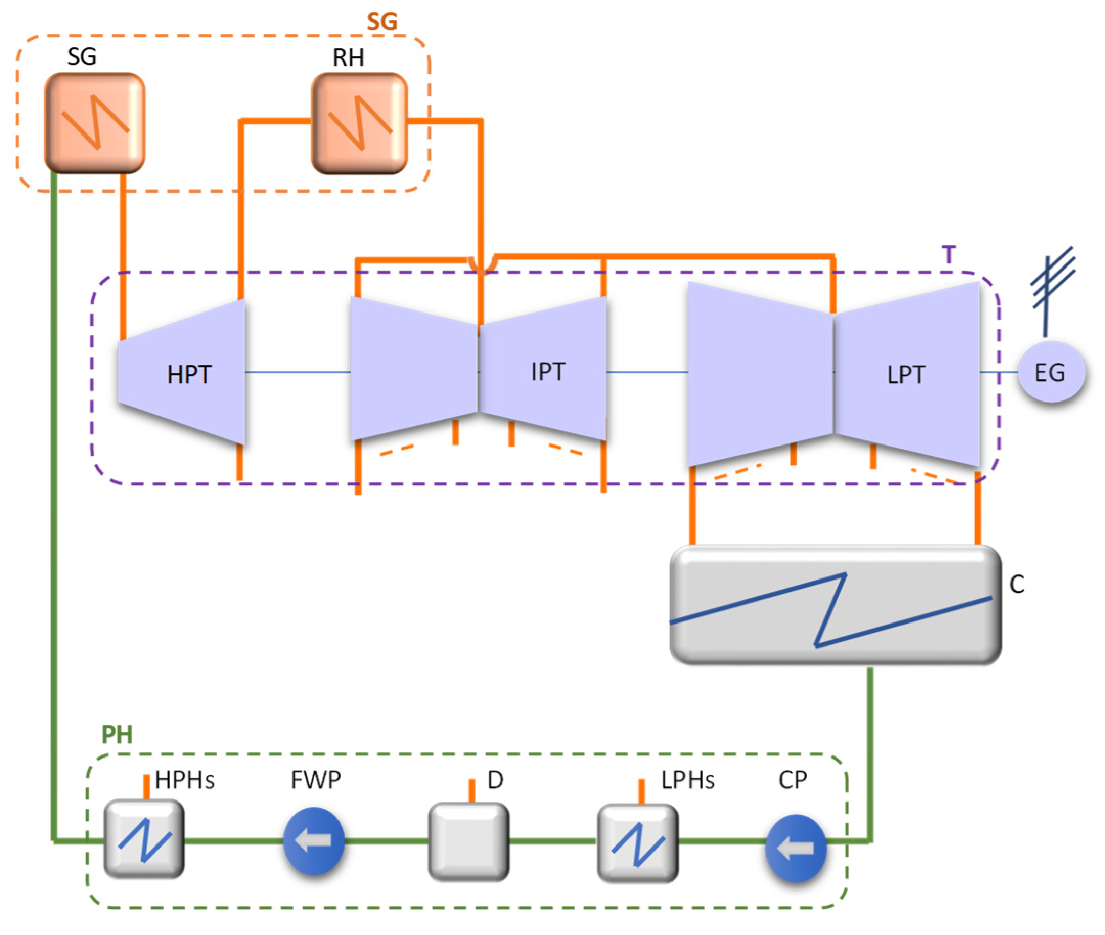
2.1. Thermodynamic Cycle Configurations
- The main steam pressure (pms, in bar) and the main steam temperature (tms, in °C);
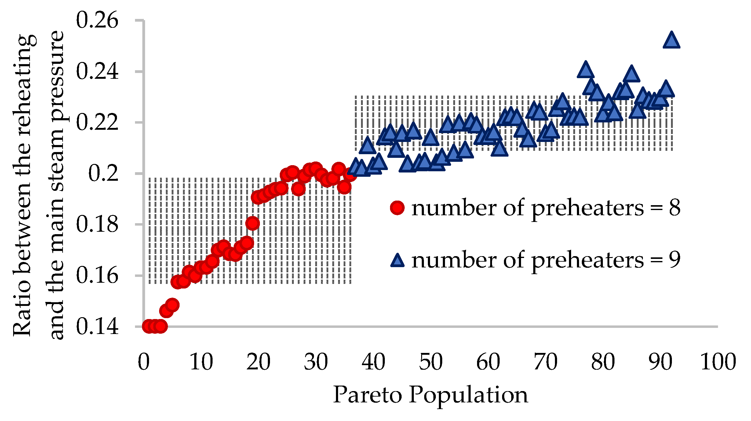
- The ratio between the reheating and the main steam pressure:
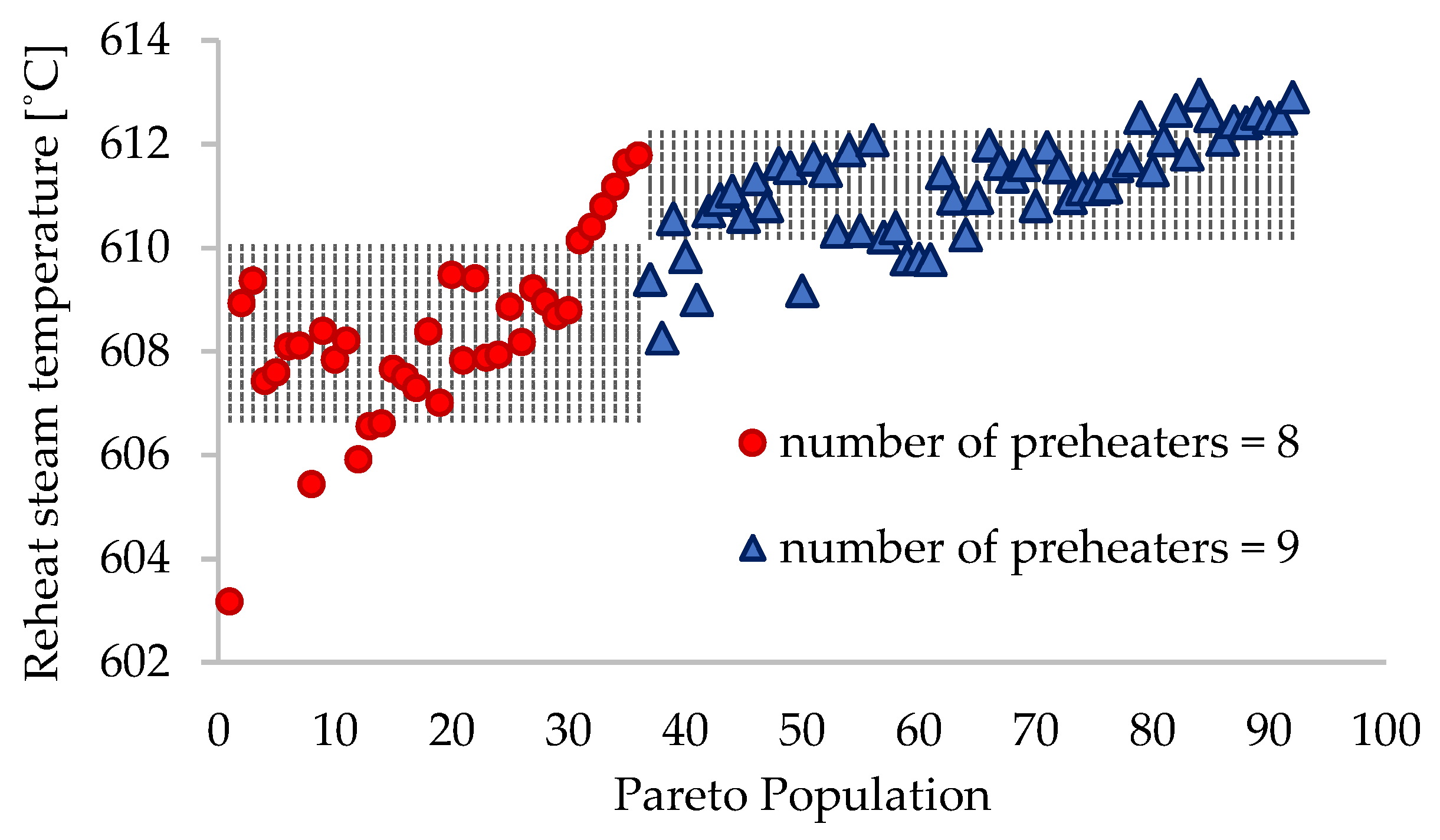
- The reheat steam temperature (trh, in °C);
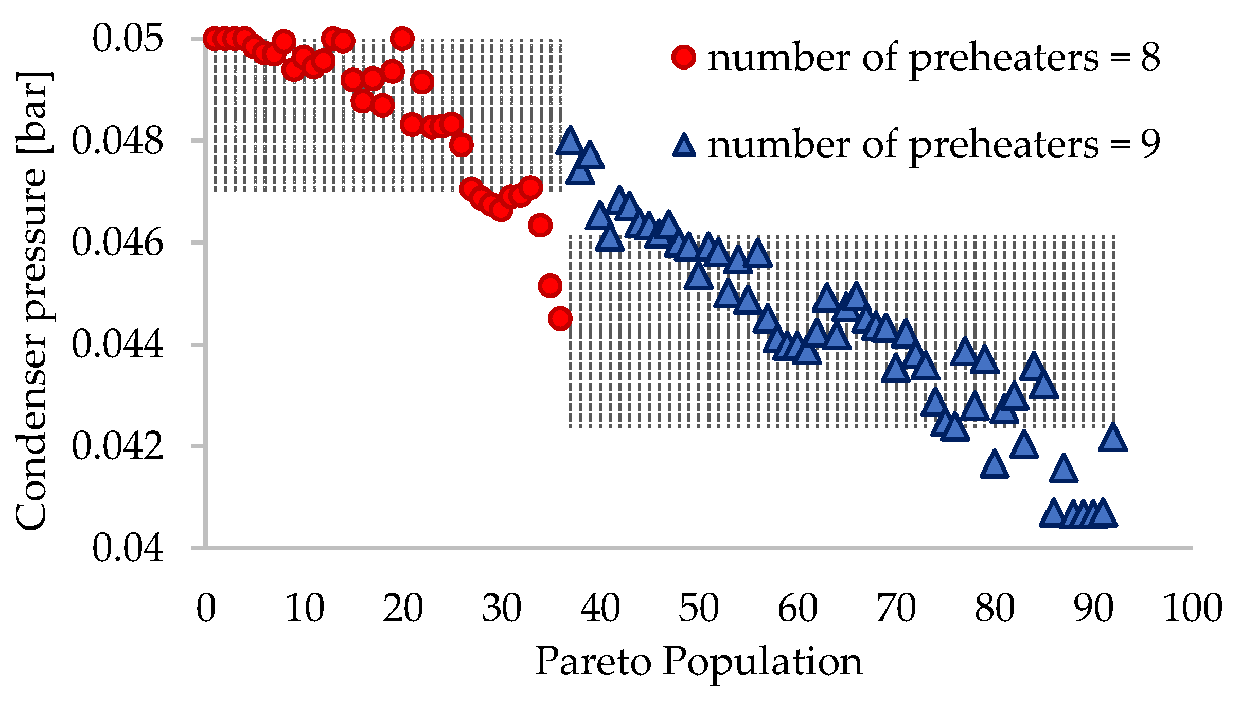
- The pressure at the condenser (pc, in bar);
- The fuel heat flow rate (Qfuel, in MW).
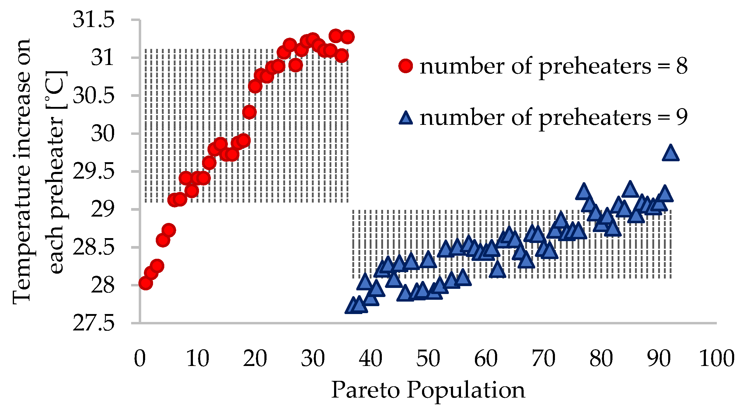
- Equal temperature increase on each preheater (Δt, in °C);
- Maximum value for Δt (maximum 32 °C);
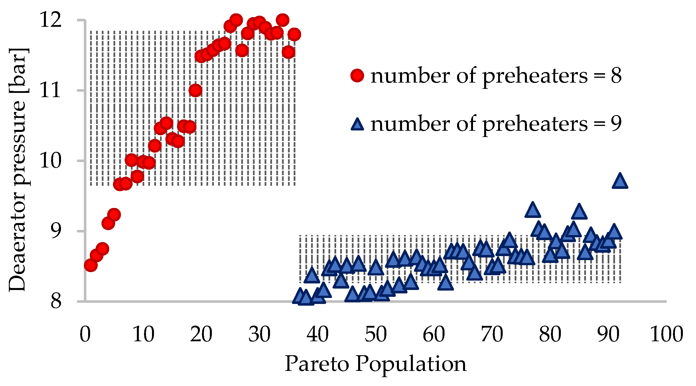
- Maximum value for the deaeration pressure (pD, in bar), (maximum 12 bar);
- Limitation of the number of HPHs by the number of LPHs (the number of HPHs should not exceed the number of LPTs);
- Restriction of the exhaust steam quality (xout, dimensionless) to avoid blades corrosion (minimum 0.88);
- The turbine is divided into several zones, defined between successive steam intakes and extractions of each cylinder, including between successive steam extractions from T;
- Variable internal isentropic efficiency through the turbine, depending on the volumetric flow rate and on the specific theoretical enthalpy reduction on the cylinder (for HPT and IPT); on the specific theoretical enthalpy reduction and on xout (for LPT);
- Imposed constant values for the overall efficiency of FWP (0.85) and PC (0.8), including their electrical motors;
- Imposed SG efficiency (0.95).
- Definition of the thermodynamic cycle configuration;
- Calculation of the thermodynamic cycle;
- Calculation of the thermodynamic cycle efficiency indicators and investment.
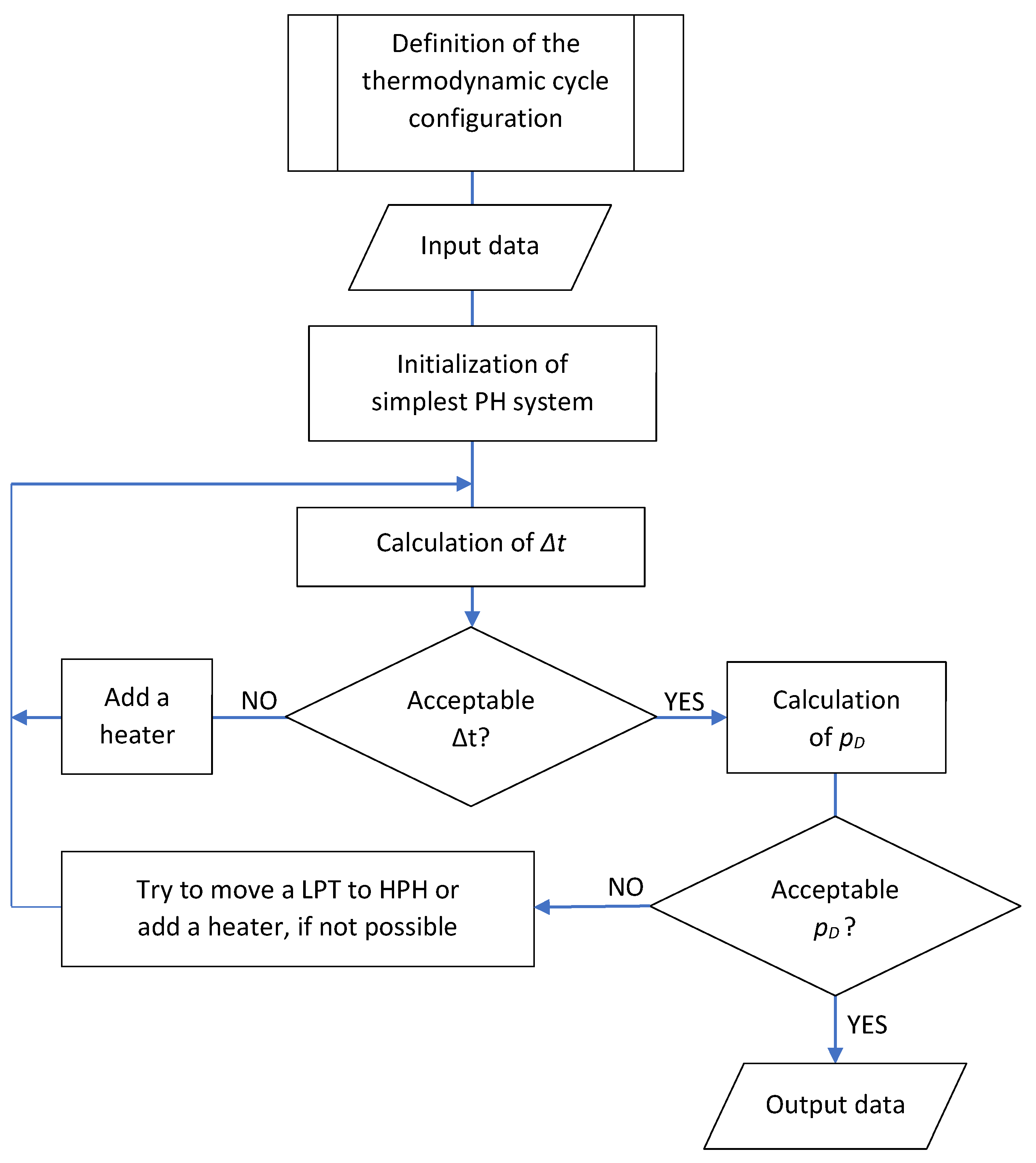
2.1.1. Definition of the Thermodynamic Cycle Configuration
2.1.2. Calculation of the Thermodynamic Cycle
2.1.3. Calculation of the Thermodynamic Cycle Efficiency Indicators and Investment
- The thermal cycle net efficiency, dimensionless [14]:
- The specific investment in power plant equipment, in USD/kW [11]:
- The specific net main steam flow rate, in kg/kWh:
- The specific net energy, in kJ/kg:
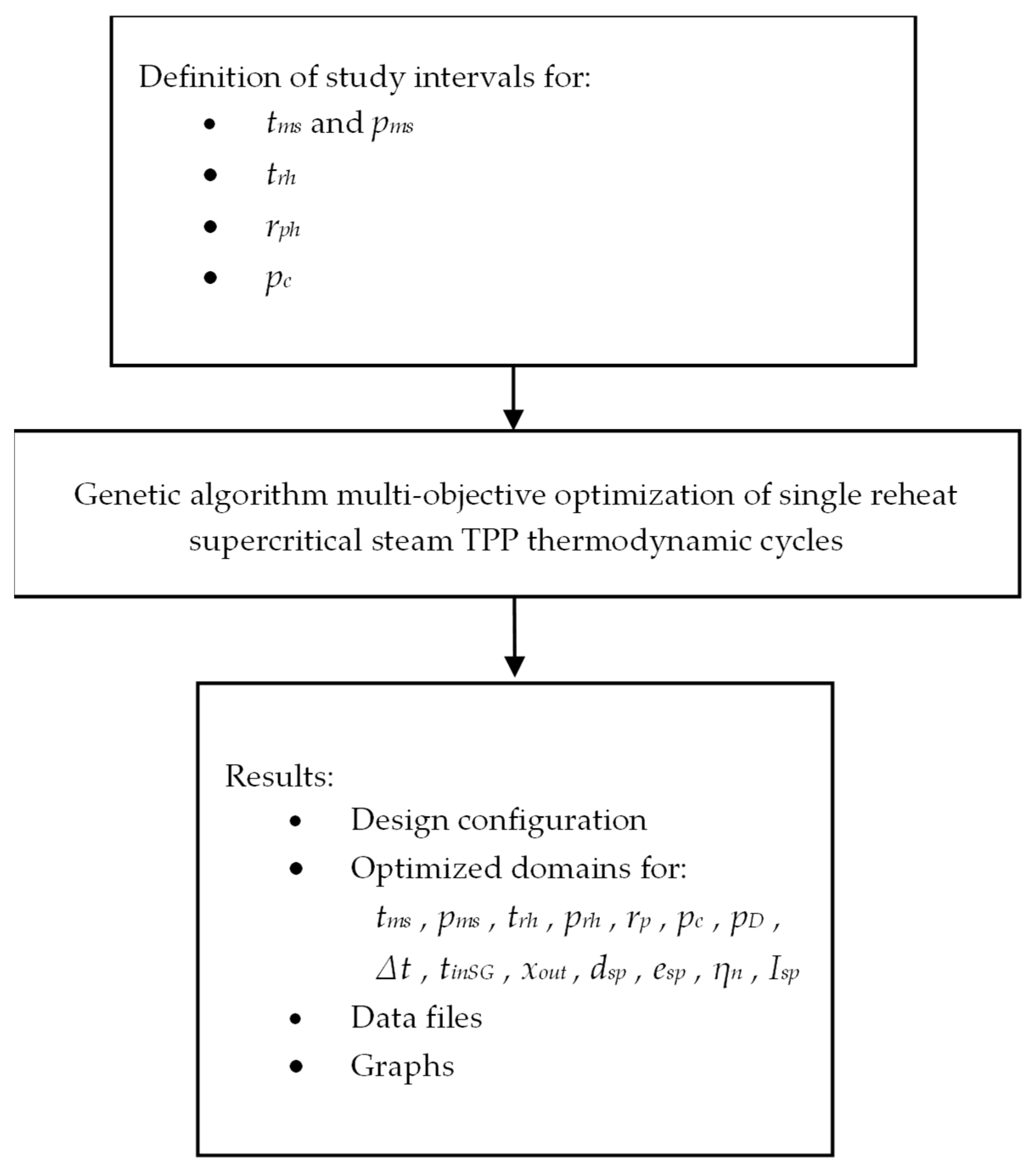
2.2. Multi-Objective Optimization
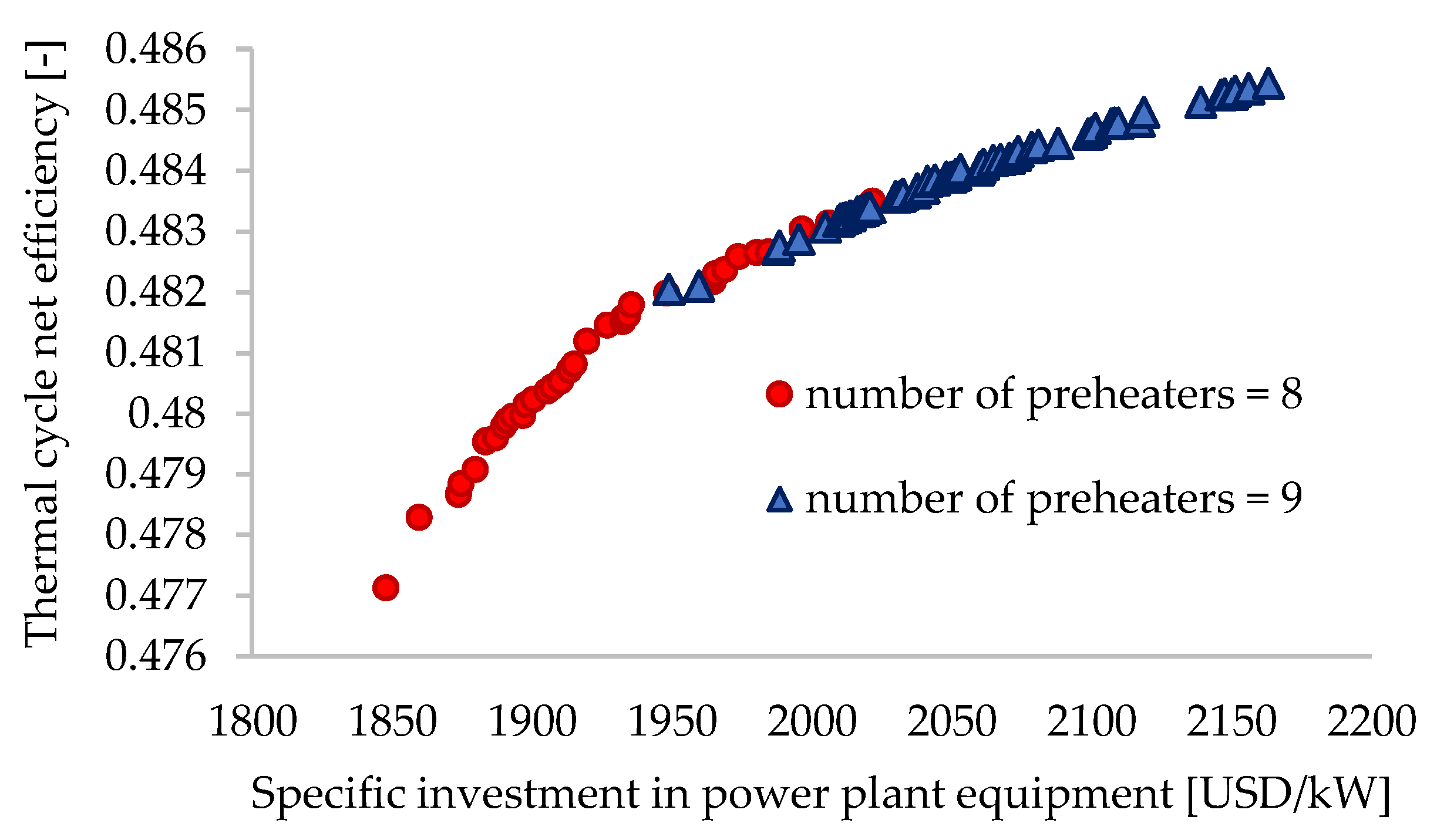
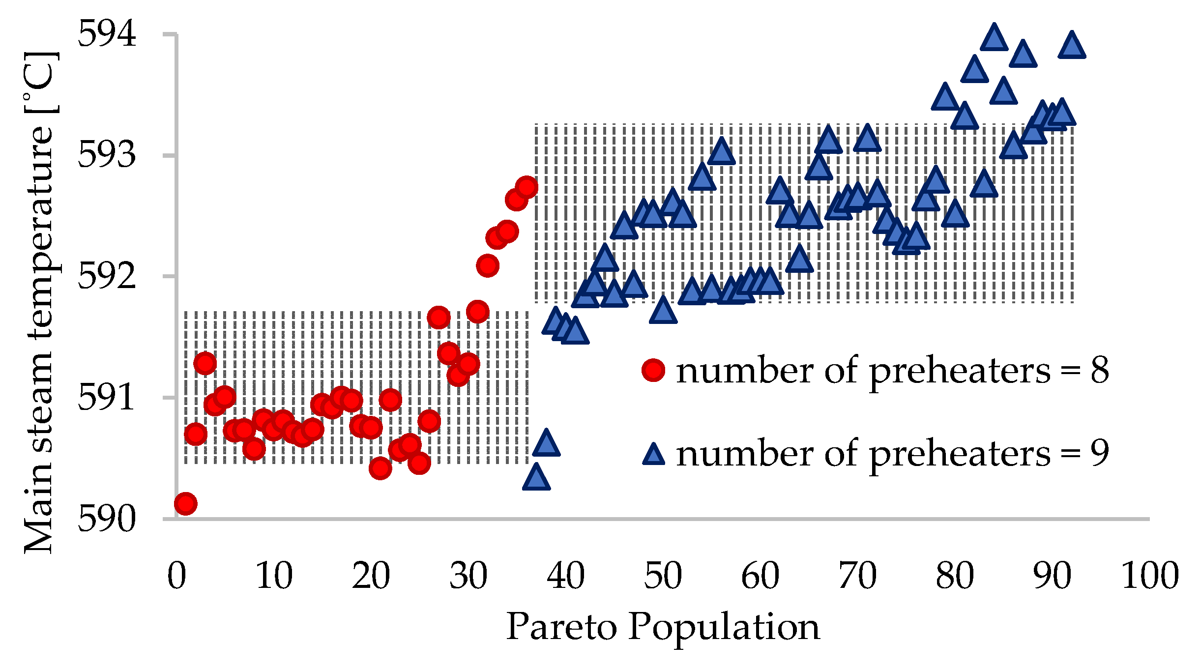
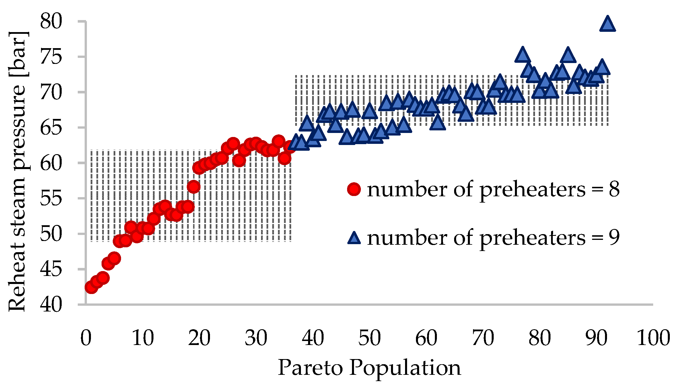
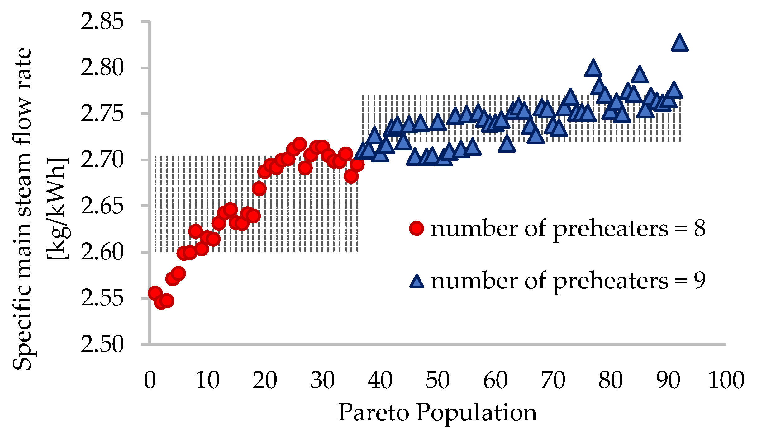
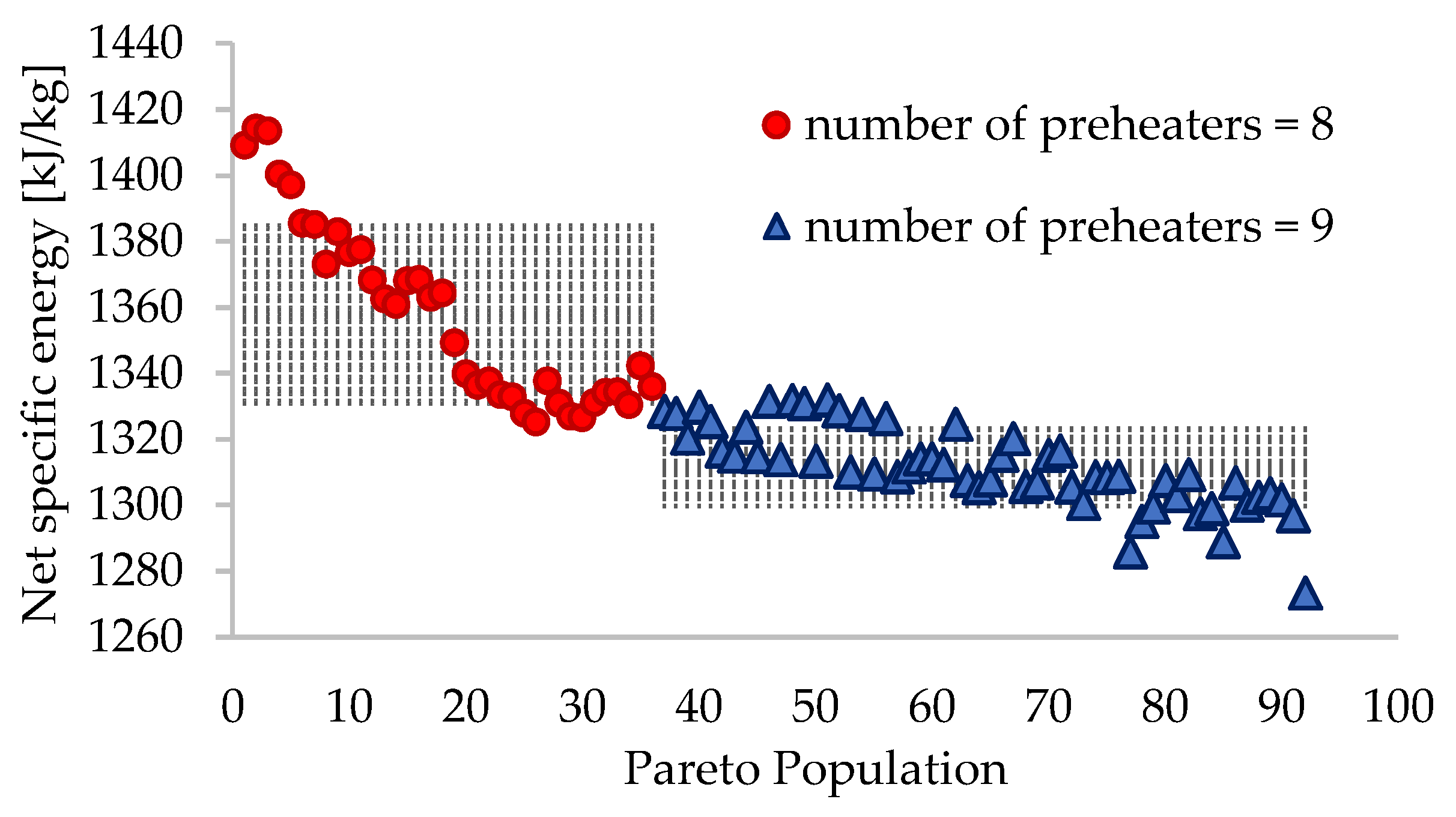
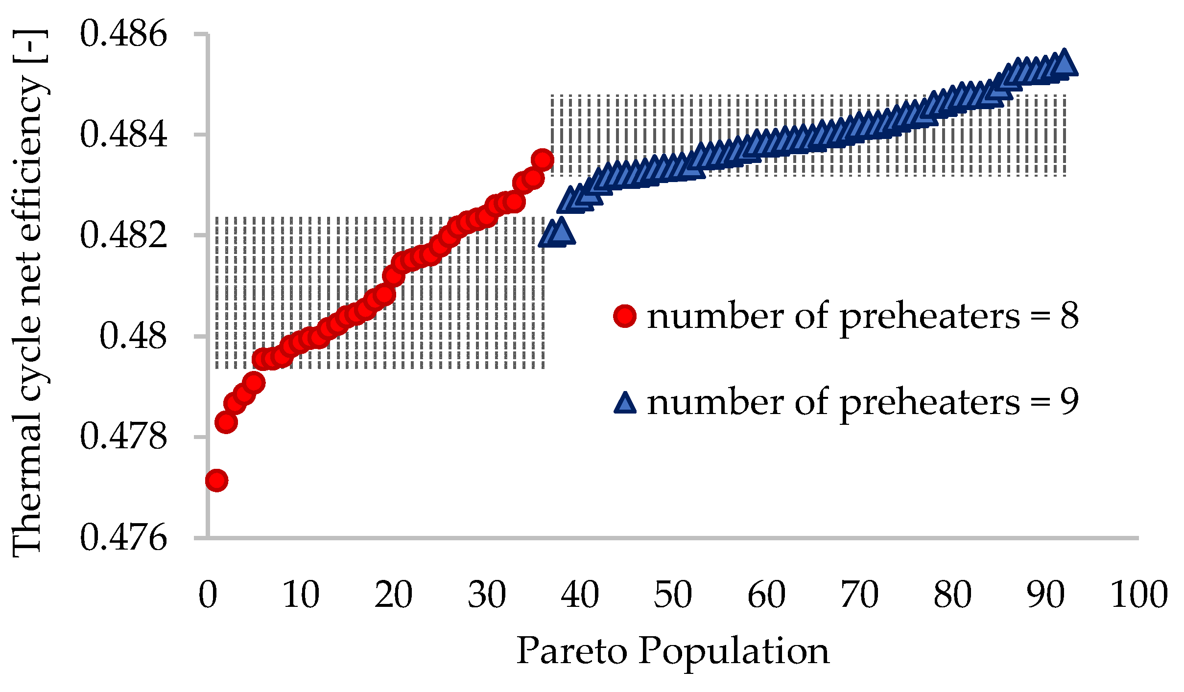
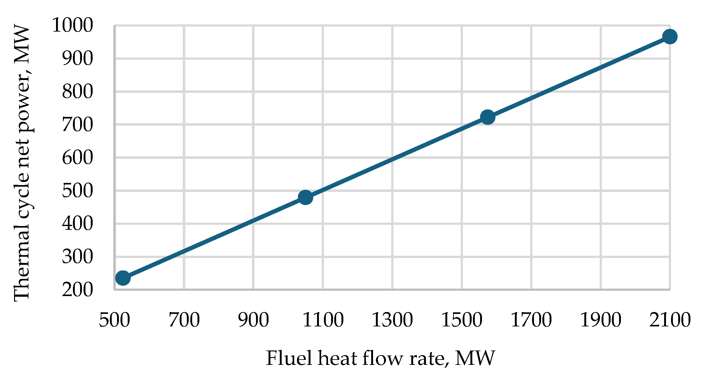
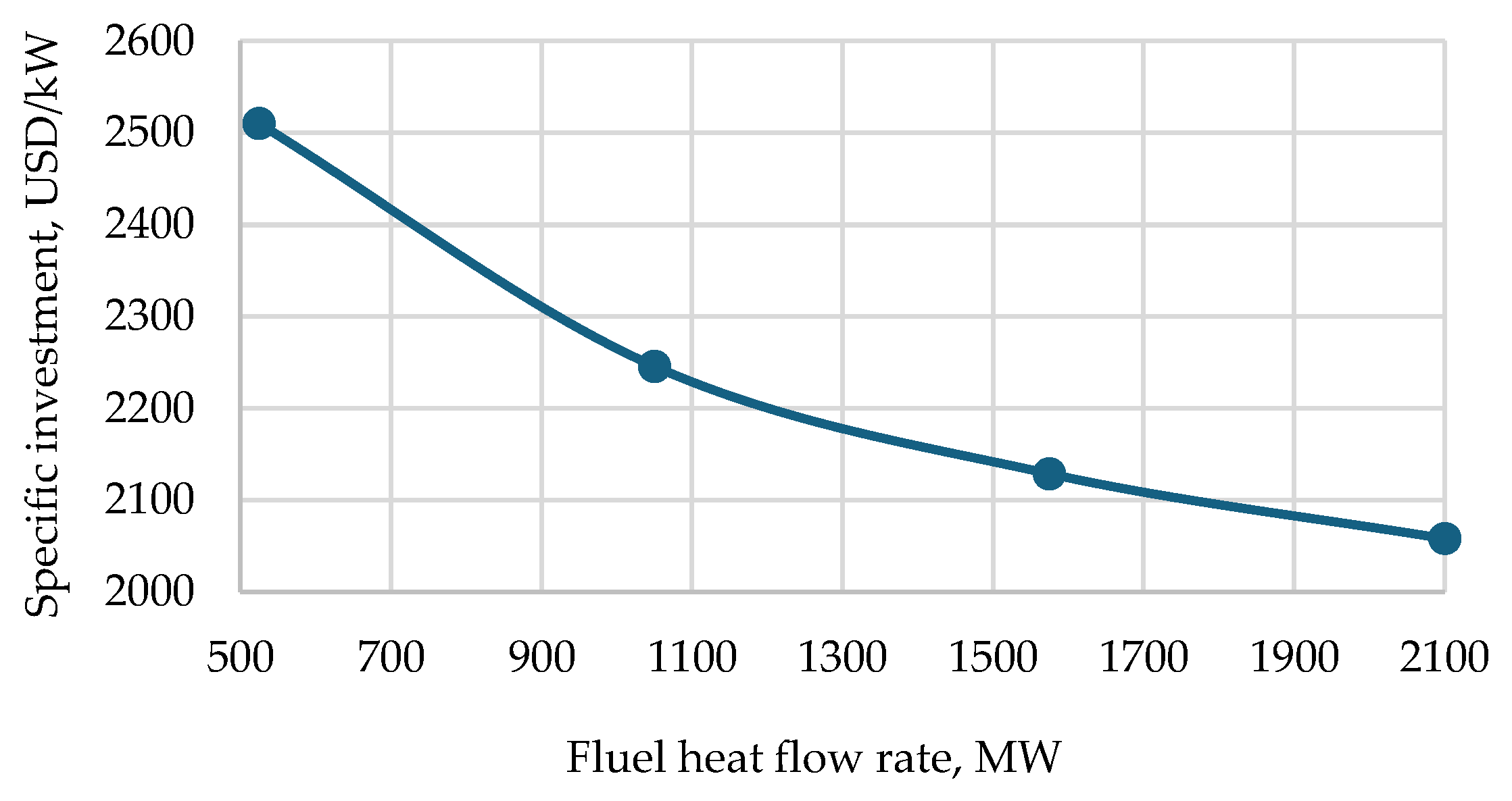
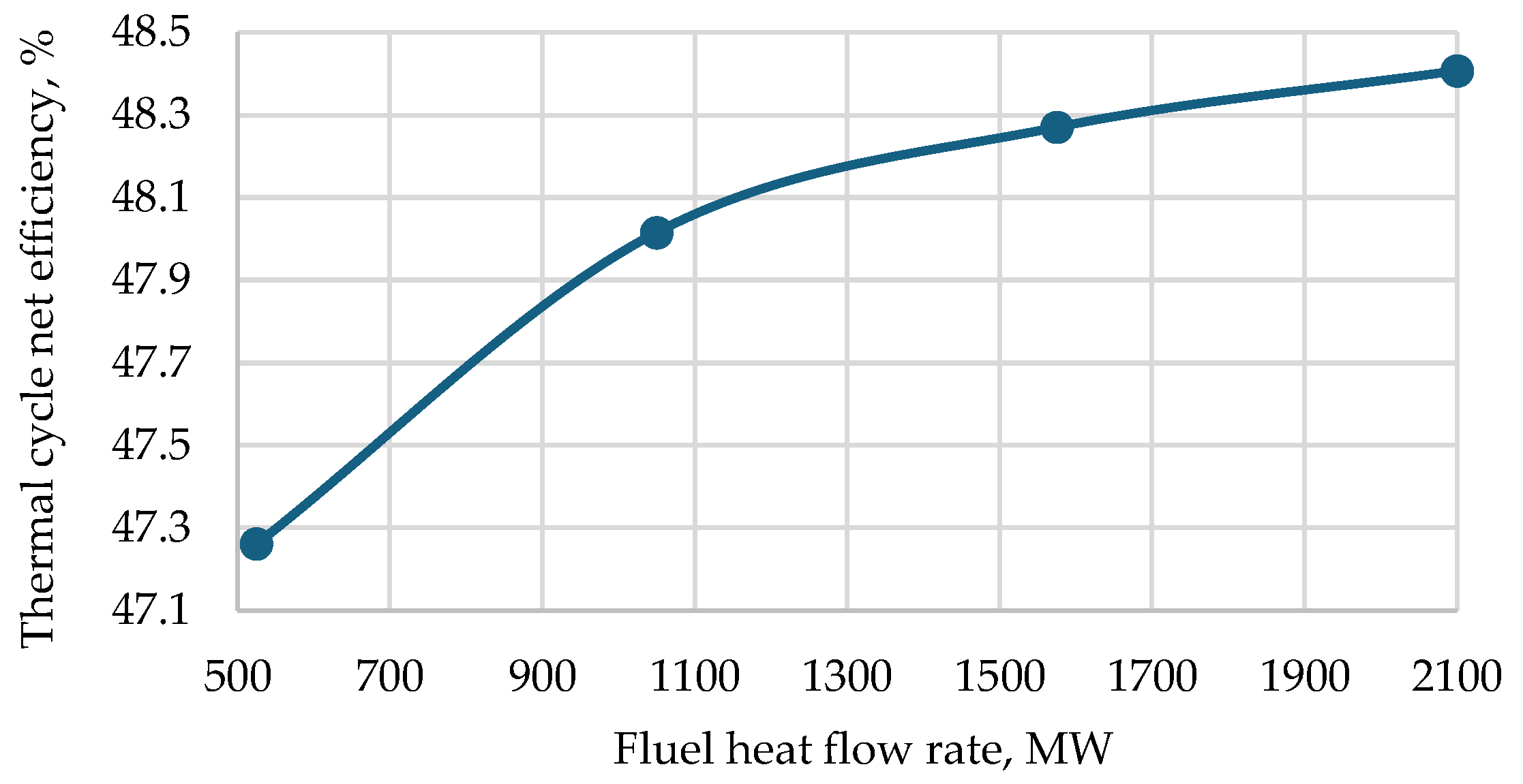
3. Results
- z = 8: ηn ∈ (47.71–48.20)% and Isp ∈ (1848–1949) USD/kW;
- z = 8, z = 9: ηn ∈ (48.20–48.35)% and Isp ∈ (1949–2021) USD/kW;
- z = 9: ηn ∈ (48.35–48.54)% and Isp ∈ (2021–2163) USD/kW.
4. Discussion
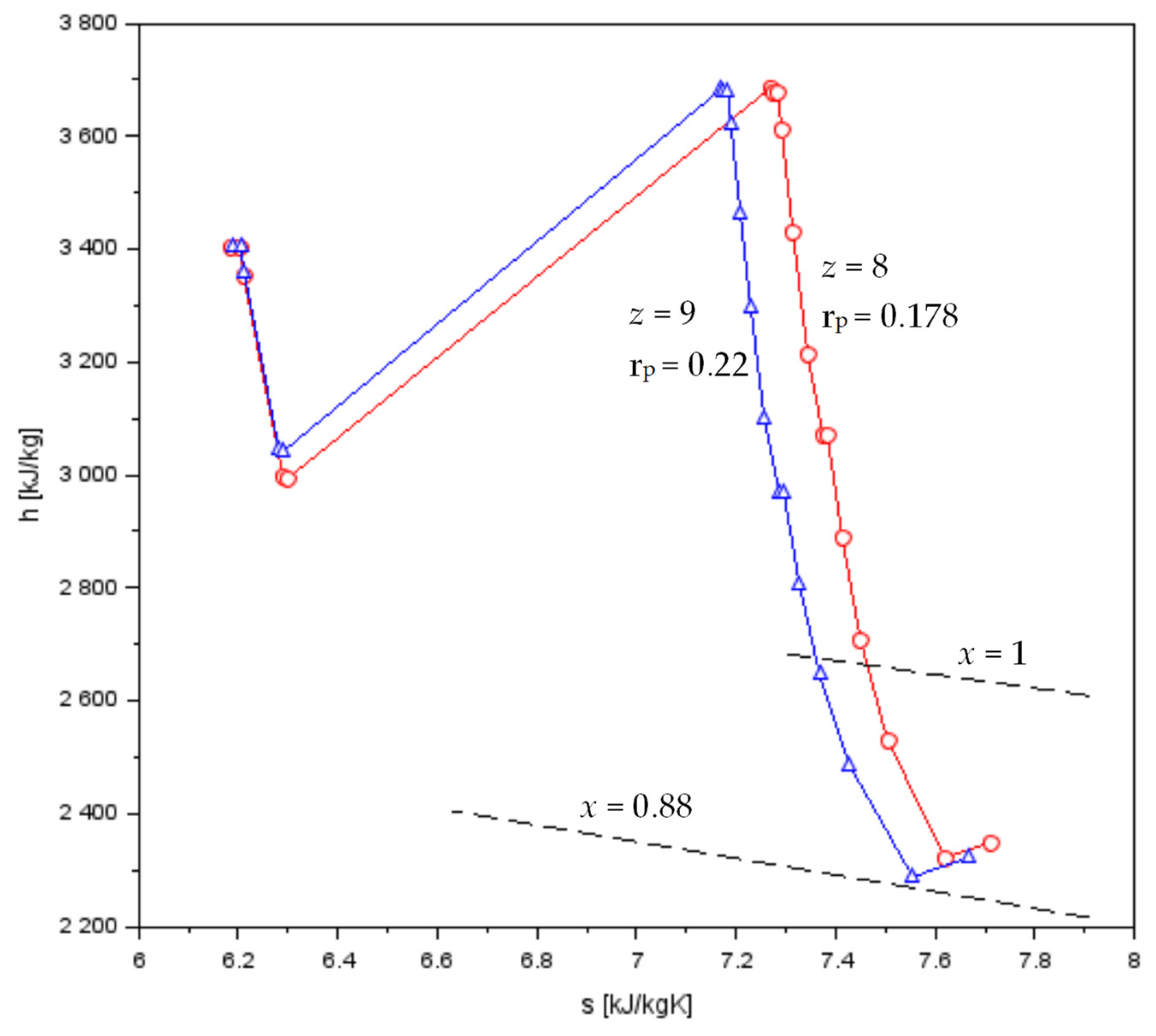
- For schemes with z = 8, rp ∈ (0.140, 0.202) bar;
- For schemes with z = 9, rp ∈ (0.202, 0.253) bar.
5. Conclusions
- For the thermal cycle efficiency, between (47.71 and 48.35)% at z = 8, and between (48.20 and 48.54)% at z = 9;
- For specific investments in the power plant’s equipment, between (1848 and 2021) USD/kW at z = 8, and between (1949 and 2163) USD/kW at z = 9.
- 48.09 ± 0.16 at z = 8, and 48.40 ± 0.09 at z = 9, for the thermal cycle efficiency;
- 1924 ± 44 USD/kW at z = 8, and 2059 ± 52 USD/kW at z = 9, for specific investments in the power plant’s equipment.
Author Contributions
Funding
Data Availability Statement
Conflicts of Interest
References
- Liu, Y.; Li, Q.; Duan, X.; Zhang, Y.; Yang, Z.; Che, D. Thermodynamic analysis of a modified system for a 1000 MW single reheat ultra-supercritical thermal power plant. Energy 2018, 145, 25–37. [Google Scholar] [CrossRef]
- Chen, X.; Shi, Z.; Zhang, Z.; Zhu, M.; Oko, E.; Wu, X. Dynamic modeling and comprehensive analysis of an ultra-supercritical coal-fired power plant integrated with post-combustion carbon capture system and molten salt heat storage. Energy 2024, 308, 132961. [Google Scholar] [CrossRef]
- Gonzalez-Salazar, M.A.; Kirsten, T.; Prchlik, L. Review of the operational flexibility and emissions of gas-and coal-fired power plants in a future with growing renewables. Renew. Sustain. Energy Rev. 2018, 82, 1497–1513. [Google Scholar] [CrossRef]
- Lin, X.; Li, Q.; Wang, L.; Guo, Y.; Liu, Y. Thermo-economic analysis of typical thermal systems and corresponding novel system for a 1000 MW single reheat ultra-supercritical thermal power plant. Energy 2020, 201, 117560. [Google Scholar] [CrossRef]
- Li, Y.; Liu, J.; Huang, G. Pressure Drop Optimization of the Main Steam and Reheat Steam System of a 1000 MW Secondary Reheat Unit. Energies 2022, 15, 3279. [Google Scholar] [CrossRef]
- Chi, S.; Luan, T.; Liang, Y.; Hu, X.; Gao, Y. Analysis and Evaluation of Multi-Energy Cascade Utilization System for Ultra-Supercritical Units. Energies 2020, 13, 3969. [Google Scholar] [CrossRef]
- Martelli, E.; Alobaid, F.; Elsido, C. Design Optimization and Dynamic Simulation of Steam Cycle Power Plants: A Review. Front. Energy Res. 2021, 9, 676969. [Google Scholar] [CrossRef]
- Tunckaya, Y.; Koklukaya, E. Comparative prediction analysis of 600 MWe coal-fired power plant production rate using statistical and neural-based models. J. Energy Inst. 2015, 88, 11–18. [Google Scholar] [CrossRef]
- Wu, X.; Shen, J.; Li, Y.; Lee, K.Y. Fuzzy modeling and predictive control of superheater steam temperature for power plant. ISA Trans. 2015, 56, 241–251. [Google Scholar] [CrossRef]
- Hou, G.; Xiong, J.; Zhou, G.; Gong, L.; Huang, C.; Wang, S. Coordinated Control System Modeling of Ultra-Supercritical Unit based on a New Fuzzy Neural Network. Energy 2021, 234, 121231. [Google Scholar] [CrossRef]
- Kler, A.M.; Zharkov, P.; Epishkin, N.O. Parametric optimization of supercritical power plants using gradient methods. Energy 2019, 189, 116230. [Google Scholar] [CrossRef]
- Lachenmaier, N.; Baumgärtner, D.; Schiffer, H.-P.; Kech, J. Gradient-Free and Gradient-Based Optimization of a Radial Turbine. Int. J. Turbomach. Propuls. Power 2020, 5, 14. [Google Scholar] [CrossRef]
- Roumpedakis, T.C.; Fostieris, N.; Braimakis, K.; Monokrousou, E.; Charalampidis, A.; Karellas, S. Techno-Economic Optimization of Medium Temperature Solar-Driven Subcritical Organic Rankine Cycle. Thermo 2021, 1, 77–105. [Google Scholar] [CrossRef]
- Opriș, I.; Cenușă, V.E. Parametric and heuristic optimization of multiple schemes with double-reheat ultra-supercritical steam power plants. Energy 2023, 266, 126454. [Google Scholar] [CrossRef]
- Cenușă, V.E.; Opriș, I. Design optimization of cogeneration steam power plants with supercritical parameters. Sustain. Energy Technol. Assess. 2024, 64, 103727. [Google Scholar] [CrossRef]
- Chen, C.; Liu, M.; Li, M.; Wang, Y.; Wang, C.; Yan, J. Digital twin modeling and operation optimization of the steam turbine system of thermal power plants. Energy 2024, 290, 129969. [Google Scholar] [CrossRef]
- Choi, H.; Choi, Y.; Moon, U.-C.; Lee, K.Y. Supplementary Control of Conventional Coordinated Control for 1000 MW Ultra-Supercritical Thermal Power Plant Using One-Step Ahead Control. Energies 2023, 16, 6197. [Google Scholar] [CrossRef]
- Wang, D.; Liu, D.; Wang, C.; Zhou, Y.; Li, X.; Yang, M. Flexibility improvement method of coal-fired thermal power plant based on the multi-scale utilization of steam turbine energy storage. Appl. Energy 2022, 239, 122301. [Google Scholar] [CrossRef]
- Wang, Z.; Liu, M.; Yan, H.; Zhao, Y.; Yan, J. Improving flexibility of thermal power plant through control strategy optimization based on orderly utilization of energy storage. Appl. Therm. Eng. 2024, 240, 122231. [Google Scholar] [CrossRef]
- Li, D.; Wang, J. Study of supercritical power plant integration with high temperature thermal energy storage for flexible operation. J. Energy Storage 2018, 20, 140–152. [Google Scholar] [CrossRef]
- Abdel-Dayem, A.M.; Hawsawi, Y.M. Feasibility study using TRANSYS modelling of integrating solar heated feed water to a co-generation steam power plant. Case Stud. Therm. Eng. 2022, 39, 102396. [Google Scholar] [CrossRef]
- Hentschel, J.; Zindler, H.; Spliethoff, H. Modelling and transient simulation of a supercritical coal-fired power plant: Dynamic response to extended secondary control power output. Energy 2017, 137, 927–940. [Google Scholar] [CrossRef]
- Panowski, M.; Zarzycki, R.; Kobyłecki, R. Conversion of steam power plant into cogeneration unit-case study. Energy 2021, 231, 120872. [Google Scholar] [CrossRef]
- Kowalczyk, Ł.; Elsner, W.; Niegodajew, P.; Marek, M. Gradient-free methods applied to optimisation of advanced ultra-supercritical power plant. Appl. Therm. Eng. 2016, 96, 200–208. [Google Scholar] [CrossRef]
- Wang, Z.; Gu, Y.; Liu, H.; Li, C. Optimizing thermal–electric load distribution of largescale combined heat and power plants based on characteristic day. Energy Convers. Manag. 2021, 248, 114792. [Google Scholar] [CrossRef]
- Marx-Schubach, T.; Schmitz, G. Modeling and simulation of the start-up process of coal fired power plants with post-combustion CO2 capture. Int. J. Greenh. Gas Control 2019, 87, 44–57. [Google Scholar] [CrossRef]
- Mohamed, O.; Khalil, A.; Wang, J. Modeling and Control of Supercritical and Ultra-Supercritical Power Plants: A Review. Energies 2020, 13, 2935. [Google Scholar] [CrossRef]
- Opriș, I.; Cenușă, V.E.; Norisor, M.; Darie, G.; Alexe, F.; Costinas, S. Parametric optimization of the thermodynamic cycle design for supercritical steam power plants. Energy Convers. Manag. 2020, 208, 112587. [Google Scholar] [CrossRef]
- Nikolaidis, P. Mixed Thermal and Renewable Energy Generation Optimization in Non-Interconnected Regions via Boolean Mapping. Thermo 2024, 4, 445–460. [Google Scholar] [CrossRef]
- Barthwal, M.; Dhar, A.; Powar, S. The techno-economic and environmental analysis of genetic algorithm (GA) optimized cold thermal energy storage (CTES) for air-conditioning applications. Appl. Energy 2021, 283, 116253. [Google Scholar] [CrossRef]
- Liu, X.; Sun, J.; Zheng, L.; Wang, S.; Liu, Y.; Wei, T. Parallelization and Optimization of NSGA-II on Sunway TaihuLight System. IEEE Trans. Parallel. Distrib. Syst. 2021, 32, 975–987. [Google Scholar] [CrossRef]
- Scilab Enterprises. Scilab 6.1.1. Available online: https://www.scilab.org/ (accessed on 14 April 2020).
- Zhao, Y.; Liu, M.; Wang, C.; Li, X.; Chong, D.; Yan, J. Increasing operational flexibility of supercritical coal-fired power plants by regulating thermal system configuration during transient processes. Appl. Energy 2018, 228, 2375–2386. [Google Scholar] [CrossRef]
- Wang, C.; Liu, M.; Li, B.; Liu, Y.; Yan, J. Thermodynamic analysis on the transient cycling of coal-fired power plants: Simulation study of a 660 MW supercritical unit. Energy 2017, 122, 505–527. [Google Scholar] [CrossRef]
- Jiang, D.; Xu, H.; Deng, B.; Li, M.; Xiao, Z.; Zhang, N. Effect of oxygenated treatment on corrosion of the whole steam–water system in supercritical power plant. Appl. Therm. Eng. 2016, 93, 1248–1253. [Google Scholar] [CrossRef]
- Xu, G.; Hu, Y.; Tang, B.; Yang, Y.; Zhang, K.; Liu, W. Integration of the steam cycle and CO2 capture process in a decarbonization power plant. Appl. Therm. Eng. 2014, 73, 277–286. [Google Scholar] [CrossRef]
- Zhao, Y.; Liu, M.; Wang, C.; Wang, Z.; Chong, D.; Yan, J. Exergy analysis of the regulating measures of operational flexibility in super-critical coal-fired power plants during transient processes. Appl. Energy 2019, 253, 113487. [Google Scholar] [CrossRef]
- Lee, J.J.; Kang, S.Y.; Kim, T.S.; Byun, S.S. Thermo-economic analysis on the impact of improving inter-stage packing seals in a 500 MW class supercritical steam turbine power plant. Appl. Therm. Eng. 2017, 121, 974–983. [Google Scholar] [CrossRef]
- Xu, G.; Xu, C.; Yang, Y.; Fang, Y.; Zhou, L.; Zhang, K. Novel partial-subsidence tower-type boiler design in an ultra-supercritical power plant. Appl. Energy 2014, 134, 363–373. [Google Scholar] [CrossRef]
- Hanak, D.P.; Manovic, V. Calcium looping with supercritical CO2 cycle for decarbonization of coal-fired power plant. Energy 2016, 102, 343–353. [Google Scholar] [CrossRef]
- Wang, D.; Li, S.; Liu, F.; Gao, L.; Sui, J. Post combustion CO2 capture in power plant using low temperature steam upgraded by double absorption heat transformer. Appl. Energy 2018, 227, 603–612. [Google Scholar] [CrossRef]
- Xu, G.; Dong, W.; Xu, C.; Liu, Q.; Yang, Y. An integrated lignite pre-drying system using steam bleeds and exhaust flue gas in a 600 MW power plant. Appl. Therm. Eng. 2016, 107, 1145–1157. [Google Scholar] [CrossRef]
- Łukowicz, H.; Bartela, Ł.; Gładysz, P.; Qvist, S. Repowering a Coal Power Plant Steam Cycle Using Modular Light-Water Reactor Technology. Energies 2023, 16, 3083. [Google Scholar] [CrossRef]
- Stępczyńska-Drygas, K.; Łukowicz, H.; Dykas, S. Calculation of an advanced ultra-supercritical power unit with CO2 capture installation. Energy Convers. Manag. 2013, 74, 201–208. [Google Scholar] [CrossRef]
- Lee, S.H.; Lee, T.H.; Jeong, S.M.; Lee, J.M. Economic analysis of a 600 mwe ultra supercritical circulating fluidized bed power plant based on coal tax and biomass co-combustion plans. Renew. Energ. 2019, 138, 121–127. [Google Scholar] [CrossRef]
- Taler, J.; Zima, W.; Ocłoń, P.; Grądziel, S.; Taler, D.; Cebula, A.; Jaremkiewicz, M.; Korzeń, A.; Cisek, P.; Kaczmarski, K.; et al. Mathematical model of a supercritical power boiler for simulating rapid changes in boiler thermal loading. Energy 2019, 175, 580–592. [Google Scholar] [CrossRef]
- Yuan, R.; Liu, M.; Chen, W.; Yan, J. CO2 emission characteristics modeling and low-carbon scheduling of thermal power units under peak shaving conditions. Fuel 2024, 373, 132339. [Google Scholar] [CrossRef]


| Parameter | Unit | Variation Domain |
|---|---|---|
| pms | bar | 300–320 |
| tms | °C | 590–610 |
| t rh | °C | 590–630 |
| rph | - | 0.14–0.36 |
| pc | bar | 0.04–0.05 |
| Parameters and Results | Units | Mean Value ± Standard Deviation (SD) | ||
|---|---|---|---|---|
| z = 8 | z = 9 | |||
| Main steam pressure | pms | bar | 312.1 ± 2.1 | 313.3 ± 1.4 |
| Main steam temperature | tms | °C | 591.1 ± 0.7 | 592.5 ± 0.8 |
| Condenser pressure | pc | bar | 0.049 ± 0.002 | 0.044 ± 0.002 |
| Deaerator pressure | pD | bar | 10.7 ± 1.1 | 8.6 ± 0.4 |
| Reheat steam pressure | prh | bar | 55.4 ± 6.5 | 68.8 ± 3.6 |
| Reheat steam temperature | trh | °C | 608.3 ± 1.8 | 611.2 ± 1.1 |
| Ratio between prh and pms | rp | - | 0.178 ± 0.021 | 0.220 ± 0.011 |
| Number of HPHs | zHPH | - | 3 | 4 |
| Number of LPHs | zLPH | - | 4 | 4 |
| Temperature increase on each preheater | Δt | °C | 30.1 ± 1.1 | 28.5 ± 0.5 |
| Exhaust steam quality | xout | - | 0.913 ± 0.004 | 0.903 ± 0.003 |
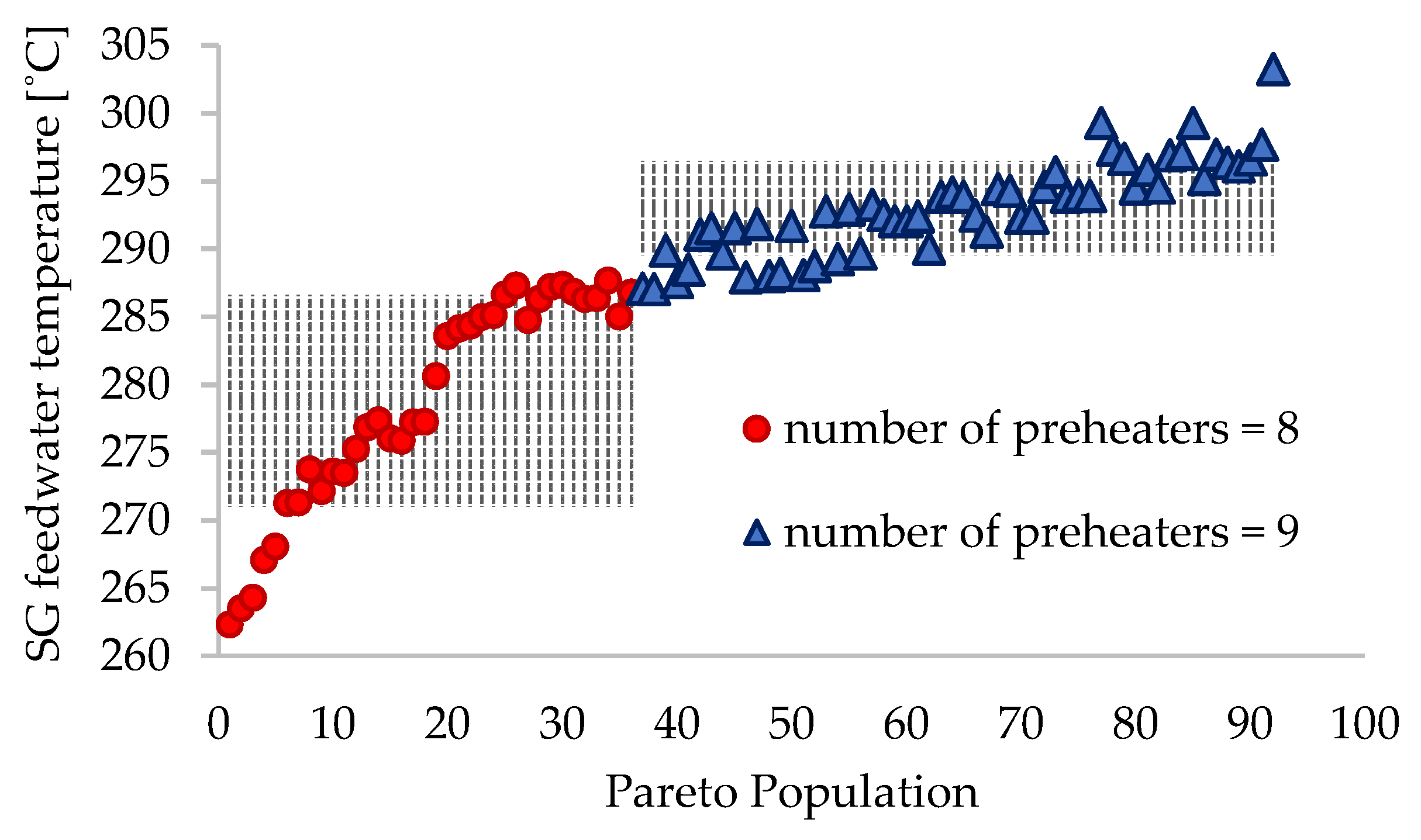
| SG feedwater temperature | tinSG | °C | 278.8 ± 7.9 | 293.0 ± 3.5 |
| Specific main steam flow rate | dsp | kg/kWh | 2.65 ± 0.06 | 2.75 ± 0.03 |
| Net specific energy | esp | kJ/kg | 1358 ± 28 | 1312 ± 13 |
| Specific investment | Isp | USD/kW | 1924 ± 44 | 2059 ± 52 |
| Thermal cycle net efficiency | ηn | % | 48.09 ± 0.16 | 48.40 ± 0.09 |
Disclaimer/Publisher’s Note: The statements, opinions and data contained in all publications are solely those of the individual author(s) and contributor(s) and not of MDPI and/or the editor(s). MDPI and/or the editor(s) disclaim responsibility for any injury to people or property resulting from any ideas, methods, instructions or products referred to in the content. |
© 2025 by the authors. Licensee MDPI, Basel, Switzerland. This article is an open access article distributed under the terms and conditions of the Creative Commons Attribution (CC BY) license (https://creativecommons.org/licenses/by/4.0/).
Share and Cite
Cenușă, V.-E.; Opriș, I. Optimal Design Parameters for Supercritical Steam Power Plants. Thermo 2025, 5, 1. https://doi.org/10.3390/thermo5010001
Cenușă V-E, Opriș I. Optimal Design Parameters for Supercritical Steam Power Plants. Thermo. 2025; 5(1):1. https://doi.org/10.3390/thermo5010001
Chicago/Turabian StyleCenușă, Victor-Eduard, and Ioana Opriș. 2025. "Optimal Design Parameters for Supercritical Steam Power Plants" Thermo 5, no. 1: 1. https://doi.org/10.3390/thermo5010001
APA StyleCenușă, V.-E., & Opriș, I. (2025). Optimal Design Parameters for Supercritical Steam Power Plants. Thermo, 5(1), 1. https://doi.org/10.3390/thermo5010001