Article

Ergodic Algorithmic Model (EAM), with Water as Implicit Solvent, in Chemical, Biochemical, and Biological Processes

Department of Food and Drug, University of Parma, I-43124 Parma, Italy
*
Author to whom correspondence should be addressed.
Thermo 2021, 1(3), 361-375; https://doi.org/10.3390/thermo1030022
Submission received: 29 October 2021 / Revised: 23 November 2021 / Accepted: 26 November 2021 / Published: 30 November 2021

Abstract

:
For many years, we have devoted our research to the study of the thermodynamic properties of hydrophobic hydration processes in water, and we have proposed the Ergodic Algorithmic Model (EAM) for maintaining the thermodynamic properties of any hydrophobic hydration reaction at a constant pressure from the experimental determination of an equilibrium constant (or other potential functions) as a function of temperature. The model has been successfully validated by the statistical analysis of the information elements provided by the EAM model for about fifty compounds. The binding functions are convoluted functions, RlnKeq = {f(1/T)* g(T)} and RTlnKeq = {f(T)* g(lnT)}, where the primary linear functions f(1/T) and f(T) are modified and transformed into parabolic curves by the secondary functions g(T) and g(lnT), respectively. Convoluted functions are consistent with biphasic dual-structure partition function, {DS-PF} = {M-PF} ∙ {T-PF} ∙ {ζw}, composed by ({M-PF} (Density Entropy), {T-PF}) (Intensity Entropy), and w} (implicit solvent). In the present paper, after recalling the essential aspects of the model, we outline the importance of considering the solvent as “implicit” in chemical and biochemical reactions. Moreover, we compare the information obtained by computer simulations using the models till now proposed with “explicit” solvent, showing the mess of information lost without considering the experimental approach of the EAM model.

1. Introduction

We accept in advance the suggestion of Lambert [1,2], who led a campaign against the theory which considers entropy as a parameter of disorder of the system. According to Lambert, entropy is a parameter of energy dispersion. It can be considered a parameter of disorder in as much as disorder is associated with energy. For instance, the sand of a beach is completely disordered unless at zero entropy, because there is no energy. By accepting the proposal of Lambert, we agree to defining free energy as a sum of two terms, Intensity Entropy (−ΔH/T) and Density Entropy (ΔS). The former function indicates the dispersion of energy produced by increasing temperature, T, which increases the velocity of the molecules, while the latter function indicates the dispersion of energy by increasing the dilution of the chemical species. We analysed the thermodynamic properties of hydrophobic hydration processes in water in a set of articles [3,4,5,6,7,8,9] and proposed the Ergodic Algorithmic Model (EAM) for maintaining the thermodynamic properties of any hydrophobic hydration reaction at a constant pressure.
If we want to obtain the thermodynamic functions of a chemical process, we plot the experimental data of an equilibrium constant RlnKdual, or other potential function RlnKeq, measured at different temperatures, as the function of (1/T), obtaining the convoluted parabolic binding function α) RlnKdual = {f(1/T)* g(T)}. If we plot the values of RTlnKdual as the function of T we obtain the convoluted parabolic binding function β) RTlnKdual = {f(T)* g(lnT)}. The binding functions are convoluted functions, where the primary linear functions f(1/T)and f(T)are modified and transformed into parabolic curves by the secondary functions g(T) and g(lnT), respectively. The constant factor R (gas constant) is introduced as a normalisation constant, to guarantee that we are referring to an Avogadro number of particles. Convoluted functions are consistent with biphasic dual-structure partition function, {DS-PF} = {M-PF} ∙ {T-PF} ∙ {ζw}, composed by ({M-PF} (Density Entropy), {T-PF}) (Intensity Entropy), and w} (Implicit Solvent). In contrast, the functions obtained by simulation methods do not consider the free energy as a thermodynamic potential function (−ΔG/RT) = (−ΔH/RT) + (ΔS/R) composed by two terms (Intensity Entropy (−ΔH/RT) and Density Entropy (ΔS/R)), specific for each hydrophobic hydration process. Simulations, referred to a conventional mono-phasic potential function or pseudo-free energy function, as proposed by other researchers, ignore the existence of the different structures of Intensity Entropy (−ΔH/RT) and Density Entropy (ΔS/R). The formal functions used in simulations are inconsistent with the dual biphasic structure of every experimental hydrophobic hydration system, with partition function composed by the product of a partition function {M-PF} ∙ {T-PF} multiplied by the partition function of the implicit solvent (w}). The list of thermodynamic information elements provided by the Ergodic Algorithmic Model (EAM) and calculated by us for about fifty compounds was analysed by statistical analysis methodologies and successfully validated [8].

Thermal Equivalent Dilution (TED): Ergodicity

The Ergodic Algorithmic Model (EAM) is a set of mathematical equations whereby it is possible to extract from a series of experimental determinations of equilibrium constants, lnK, or other equivalent potential functions measured at different temperatures, the thermodynamic properties of any hydrophobic hydration reaction, by exploiting the Thermal Equivalent Dilution (TED) principle [3,4,5,6,7,8,9]. The TED principle can be represented by the equality
nwCp,wdlnT = Rdlndid,A
where did,A = 1/xA is ideal dilution; xA is the molecular fraction of species A; Cp,w = 75.36 J K−1 mol−1 is the molar heat capacity of liquid water and R = 8.314 J·mol−1 K−1 is the gas constant. The expression in Equation (1) can be considered as the ergodicity parameter of a system.
With reference to Figure 1a, representing a series of hyperbolas:
exp(−ΔG/RT) = exp(−ΔH/RT) exp(ΔS/R)
The EAM model consists of a correct determination of the coordinates of a point A (x,y), with X = exp(ΔSA/R) and y = exp(−ΔHA/RT). By referring one equation to a given process, we choose one hyperbole of the family, corresponding to a point P on the auxiliary axis z of the diagram. Then, by choosing (Figure 1b) the value of ordinate y (exp(−ΔHA/RT)) and the value of abscissa x (exp(ΔSA/R)) of point A (or of point B, or C), we choose a point on that hyperbola, thus reaching all the information elements available. Instead, this point A (or B or C) cannot be chosen by computer simulation. This is the essential information element that we lose by employing computer simulations: we cannot fix a point referring to the specific system on the chosen hyperbola. On the auxiliary coplanar axis z, we read the scale of values of point P, exp(−ΔΓ/RT) = (exp(−ΔG/RT) cos 45°, with xP = yP. By computer simulation, we might perhaps choose the correct hyperbola P, but we cannot fix any point A for a specific reaction, losing all the essential information elements carried by the coordinates of A, −ΔHA/RT, Intensity Entropy and ΔSA/R, Density Entropy, respectively.

2. Free Energy

2.1. Thermodynamic Free Energy

The probability space of Figure 1, representing the exponential functions, generates the thermodynamic space of Figure 2 respectively, where the exponentials are represented in an orthogonal axis system. In this system, the abscissa xA represents Density Entropy and the ordinate yA represents Intensity Entropy. The hyperbolas of the exponential diagram are transformed into a set of parallel lines, orthogonal to the diagonal auxiliary axis (−ΔΓ/T) = (−ΔG/RT) (cos 45°). The coordinates of point A can be determined by experimental determination of RlnKmot = (−ΔG/T) = (−ΔH/T) + (ΔS/T), measured at different temperatures T, and analysed following the Ergodic Algorithmic Model (EAM). In contrast, computer simulations [10] might even guess (Figure 1a) the correct vector P (−ΔΓ/T), marked in blue in Figure 1a, but ignore the vectors (ΔSA) + (ΔHA/T), marked in red in Figure 2b, thus losing all the information elements carried by these vectors. Computer simulations, in search for a potential function RlnK = f(x) to represent as the function of a variable x, calculate the function
RlnK(P) = (−ΔG(P)°/RT) = (−ΔΓ/RT)/(cos 45°)
This function assumes implicitly that (−ΔH(P)/T) = (ΔS(P)) on the diagonal, thus cancelling any difference, between the enthalpy parameter (or Intensity Entropy) and the entropy parameter (or Density Entropy). The computer-simulated function, not considering the difference between the two terms, Intensity Entropy and Density Entropy, cancels all the information elements contained there, and characterises each specific reaction, A, B, or C, at points A, B, or C, respectively. By applying the Ergodic Algorithmic Model (EAM) to a set of potential parameters (e.g., RlnKdual or RTnKdual), referring to one specific hydrophobic hydration process, experimentally determined at different temperatures, one can calculate the binding functions
α) RlnKdual = {f(1/Tg(T)}
and
β) RTlnKdual = {f(Tg(lnT)}
which are “convoluted” functions. By developing the convoluted functions, one can calculate the primary motive functions, f(1/T) and f(T), respectively, of the convolution:
RlnKmot = (−ΔHmot/T) + (ΔSmot)
RTlnKmot = (−ΔH0) + (TΔSmot)
The two terms of each motive function are specific for each compound and suited to recover the information elements of each hydrophobic hydration process. Other additional important information elements are produced by analysing the secondary function g(T) and g(lnT) of each convolution, such as ±ξw, the pseudo-stoichiometric number of water molecules WI. The pseudo-stoichiometric number ±ξw is calculated from the curvature of the binding function, that is a concave function, with ΔCp,hydr = ξw Cp,w >0 for Class A, or a convex function, with ΔCp,hydr = −ξw Cp,w < 0 for Class B. ξw = |nw| is the number of water clusters WI involved in each process, and Cp,w = 75.36 J·K−1mol−1 is the molar heat capacity of liquid water.
The difference between the functions calculated by the so-called “simulation” and the convoluted binding functions obtained by applying the Ergodic Algorithmic Model (EAM) can be expressed by stating that the function calculated by simulation is lnKsimul = f(−ΔG/T), without specifying coordinates of any point A, B, or C, etc. The assignment of these equations means specifying, in the hyperbolic diagrams, the coordinates of each point, A, B, or C, each point referring to one specific different hydrophobic reaction, with specific properties and specific interrelations between properties for each family of compounds.
The complete set of equations constituting the Ergodic Algorithmic Model (EAM) are reported in Appendix A. The information elements from EAM are shown in Table 1.
The simulated calculated function RlnKsimul is not suited to the study of these systems because it refers to a model of a monophasic system, not conforming to the biphasic composition [7] with implicit solvent of diluted aqueous systems and of biological solutions. The inadequacy of the monophasic model for simulations leads to the loss of essential information elements and to a pseudo-free energy potential function.

2.2. Pseudo-Free Energy Function

C. Chipot and A. Pohorille (Eds.) [10] published a book with title: “Free Energy Calculations. Theory and Application in Chemistry and Biology”, where they treat the problem of the calculation of free energy functions lnKsimul = f(−ΔG/T). They optimize the function exp(−ΔG/RT), but forget that thermodynamic free energy should be written and calculated as
exp(−ΔG/RT) = exp(−ΔH/RT) · exp(ΔS/R)
with a distinction between the Density Entropy term (exp(ΔS/R) and Intensity Entropy term (exp(−ΔH/RT)). Therefore, the name “Free Energy Calculations” should be changed into that of “Conventional monophasic” partition function or into that of “pseudo-Free Energy” function. If one is searching for a correct free energy procedure, one should set an algorithm to calculate
(−ΔG/RT) = {∫d(−ΔH/RT) + ʃd(ΔS/R)}
where the integral ∫d(−ΔH/RT) should in principle be calculated as MD function (MD stands for molecular dynamics) and the integral ∫d(ΔS/R) should in principle be calculated as the MC function (MC stands for Monte Carlo). If one does not know these algorithms to calculate the integrals ∫d(−ΔH/RT) = << (−ΔH/RT) >> and ∫d(ΔS/R)} = << (ΔS/R) >>, one can substitute the integral functions by the definite thermodynamic functions (−ΔH/RT) and (ΔS/R), respectively, obtained by processing the experimental data, determined at different temperatures, by applying the Ergodic Algorithmic Model (EAM). This means that we can determine, in advance, the final value of the two separate integrals by processing by EAM a set of potential functions, experimentally determined at three, four or more temperatures, and, in force of the Thermal Equivalent Dilution (TED) principle, behaving as dependent upon dilution. Another point ignored by Chipot and Pohorille [10,11] is the introduction of the constant partition function ζw = 1, referring to water as an implicit solvent at constant thermodynamic potential μs.
Following the EAM procedure means cutting off all the treatments of hydrophobic processes produced according to the methods suggested by Chipot and Pohorille [10,11].
According to C. Chipot et al. [12], the methods targeted at the computation of free energy differences can be clustered into four classes:
(i)
Perturbation theory [10,11,13,14] and free energy perturbation (FEP) calculation [15,16];
(ii)
Determination of gradients and integration thereof, i.e., thermodynamic integration-like approach [17,18];
(iii)
Histograms [12,19,20,21];
(iv)
Non equilibrium work (NEW) [13,14,22,23].
Though NEW shares common theoretical foundations with FEP, the latter can be assumed as a limiting case of the former [22].
Unfortunately, none of the eminent researchers [12,13,14,16,18,20,21,22,23] active in simulation calculations have considered the thermodynamic free energy as composed by two distinct terms, Density Entropy and Intensity Entropy. On the other hand, Chipot and Pohorille and none of their followers have produced various sets of experimental data satisfying the statistical analysis and presenting mean unitary values with extremely low standard deviation. This important and decisive result was presented by us [8]. Free energy in chemical thermodynamics is set in probability space as
exp(−ΔG/RT) = exp(−ΔH/RT) · exp(ΔS/R)
and in thermodynamic space as:
(−ΔG/RT) = (−ΔH/RT) +S/R)
The partition function of Equation (10) has a typical hyperbolic structure, wherein exp(−ΔH/RT) is representative of Intensity Entropy and exp(ΔS/R) is representative of Density Entropy (Figure 1), as different distinct properties of a thermodynamic system. By choosing this free energy partition function, we accept that the thermodynamic system has a specific structure, composed of two entropic terms, i.e., Entropy Intensity and Entropy Density, respectively. These systems are constituted by a binary structure composed by a solvent at constant thermodynamic potential μs (implicit solvent) and a solution with ergodic properties. These systems are represented in probability space by a dual-structure partition function.

3. Explicit Solvent and Implicit Solvent

Chipot and Pohorille [10] assumed the model of “explicit” solvent for water for the calculation of the pseudo-free energy. The “explicit” solvent [24] for water is incompatible with the dual-structure partition function {DS-PF} = {M-PF} · {T-PF} · w} of the aqueous systems as proposed by EAM model [9]. w} represents the partition function of implicit solvent, at constant thermodynamic potential μs. These words explain the difference between pseudo-free energy calculations and the Ergodic Algorithmic Model (EAM). Pseudo-free energy calculations are applied to “explicit” solvent molecular systems, with homogenous composition whereas EAM requires an “implicit” solvent model for a dual system with biphasic composition. The dual system is composed by solvent in excess (“implicit” solvent) and diluted solute, as proved by statistical analysis of errors, extended to a large population of hydrophobic hydration processes [8]. Specifically, we assume [9] that every aqueous solution, and particularly biological solutions, has a biphasic composition, constituted by a solvent at constant potential (i.e., “implicit” solvent) and a diluted solute. None of the systems studied by perturbation theory [10,11] and by free energy perturbation (FEP) calculation [15] with determination of gradients and integration thereof, i.e., the partition function w}, give any contribution to the free energy of the whole system, conforming to the characteristics of the “implicit” solvent. The assumption of the “explicit” solvent for these systems would mean introducing a specific variable partition function for the explicit solvent. This hypothetical function should be suited to calculate a variable free energy contribution by the solvent, i.e., by the component at constant potential, whose contribution to free energy is constantly zero. In other words, we should introduce a partition function for the explicit solvent with the properties of implicit solvent, which would mean accepting the implicit solvent as the correct choice.
Notwithstanding these drawbacks, the computer simulation method called FEP (Free Energy Perturbation) [19] seems to have reached excellent results, (see Schrödinger Platform). Starting from some basic assumptions, several eminent researchers have developed a series of computer programs whereby an ingenious framework of mathematical relationships has been built up. We are dubious that these computer simulation methods are reliable.

4. Free Energy: Intensity Entropy and Density Entropy Components

We endeavour now to discover whether it is possible to create a mathematical framework, alternative to the pseudo-free energy function, with structures compatible with a structure of free energy (−ΔG/RT), considered as the sum of one Intensity Entropy term (−ΔH/RT) and one Density Entropy term (ΔS/R), with the “implicit” solvent model. The integrals ∫d(−ΔH/RT) and ∫d(ΔS/R)} of Equation (9) have the advantage that the results of the integration can be substituted by the definite values of (−ΔH/RT) and (ΔS/R), respectively, obtained from experimental determinations of appropriate potential functions, processed by the Ergodic Algorithmic Model (EAM). The results of the application of EAM are the expressions of the motive constants
RlnKmot = (−ΔHmot/T) + (ΔS0)
and
RTlnKmot = (−ΔH0) + (ΔSmot)T
(see Equations (6) and (7)). Pseudo-free energy calculations are applied to “explicit” solvent molecular systems with homogenous composition, whereas EAM requires an “implicit” solvent model for a dual system, composed by solvent in excess (implicit solvent) and diluted solute. The authors of simulations focus on the application of free energy perturbation methods utilizing MD for the calculation of protein–ligand binding affinities in structure-based drug discovery projects. The simulations consider the basic expression
ΔF(AB) = FBFA = kBT ln < exp[−(EBEA)/kBT] >
or Zwanzig equation, where T is the temperature and kB is Boltzmann’s constant. The triangular brackets < and > denote an average over a simulation run for state A. In practice, one runs a normal simulation for state A, but each time a new configuration is accepted, the energy for state B is also computed. The difference between states A and B may be in the atom types involved, in which case the ΔF obtained is for “mutating” one molecule onto another, or it may be a difference of geometry, in which case one obtains an enthalpy map along one or more reaction coordinates. In practice, the averages in Equation (14) are obtained using the so-called λ-dynamics: E(λ) = (1−λ) · EA + λ · EB, where λ changes smoothly from 0 to 1 (i.e., from state A to state B) in order to improve the sampling of states [25].

5. Procedure According to Ergodic Algorithmic Model (EAM)

The dual system of every hydrophobic hydration process is represented in EAM by a product of partition functions {DS-PF} = {M-PF} · {T-PFth} · {ζw}, whereby the Motive Partition Function {M-PF}, referring to Density Entropy, is multiplied by a thermal partition function {T-PF}, referring to Intensity Entropy, and by {ζw}, at constant potential (implicit solvent). In mathematical format, we consider a partition function
exp(–ΔGdual/RT) = {(exp(−ΔHmot/RT) (exp(ΔSmot/R)} = Kdual = Kmot·ζw
with ζw = 1. According to EAM, the integration of differential functions cannot be applied to free energy calculation because the chemical reacting component, represented by {DS-PF}, is ruled by binomial distribution, with the partition function composed by a limited sum of finite arithmetic elements. EAM, however, considers an infinitesimal statistical distribution of molecules within sublevels hj,i of each macrolevel Hi (see Figure 3).
It is possible to apply the integration to the changing of distribution of molecules among sublevels, ruled by the statistical distribution of a non-reacting subsystem. In fact, the passage from one level to another implies a redistribution of molecules among the levels Hi to Hi+1 of the transformed molecule. This level-to-level passage can be a continuous process suitable for integration. The whole reaction also involves (Figure 4) a change in the multiplicity of states and this transformation of moles can be expressed by finite numbers, suitable for mathematical finite transformation corresponding to the coefficients of chemical equation. We can consider the contributions by integration terms as producing Intensity Entropy whereas the contributions by multiplicity mathematical terms as producing Density Entropy, respectively. The question now is: how can we exploit the computer programs on the market to calculate the Ergodic Algorithmic Model?
Instead of Zwanzig Equation (16), we should employ the equation
ΔH(AB) = HBHA = kBT ln < exp(<(−HB + HA)/kBT) >
(a)
Calculation of convoluted binding functions from experimental determinations; then, by applying EAM we derive Rln Kmot.
(b)
Calculation of simulation functions according to HEP.
In the former case, the solvent is considered at constant potential, i.e., as implicit solvent, whereas in the latter case the solvent is considered as explicit solvent.
In the calculation of the simulation function, we can consider the passage from one level H0 to level H1 with a gradual change in molecular structure from one to another shape, with a change in wave function. This passage consists of a change in Intensity Entropy: the whole mole passage of Intensity Entropy corresponds to the experimental determination of −ΔH/T in the not Hoff function or similarly, in EAM to the slope of RlnKmot = −ΔH/T + ΔS. The multiplicity within each macrolevel corresponds to Density Entropy change and is measured in experimental thermodynamic space by the ΔS component and in EAM by the slope of RTlnKmot = −ΔH + T ΔS. There is correspondence between the two components of the equation −ΔG/T = −ΔH/T + ΔS and the terms calculated from the experimental data by applying RlnKmot in EAM.
The main achievements obtained by the Ergodic Algorithmic Model can be found in references [7,8,9].

6. Thermodynamic Functions and Information Elements

The development of the Ergodic Algorithmic Model (EAM) applied to a series of experimental data can show the relationships between thermodynamic functions and information elements.
The information necessary to construct the motive functions can be obtained from the definition of the primary functions f(1/T) of the binding function RlnKdual = {f(1/Tg(T)} and by the primary function f(T) of the binding function RTlndual = {f(Tg(lnT)}. The Ergodic Algorithmic Model (EAM) consists of the calculation and processing of the convoluted binding functions, to obtain the motive functions RlnKmot and RTlnKmot (Table 2). The two motive functions contain the correct information elements concerning the leading hydration process of the reaction, together with the thermodynamic properties of the chemical process associated with hydration. In carboxylic acids, for example, the reaction associated with hydration is protonation of the base.
The two binding functions RlnKdual = {f(1/Tg(T)} and RTlndual = {f(Tg(lnT)} have a parabolic shape. The sign of these binding functions is sensible to the sign of ΔCp,hydr (Figure 5).
The correct procedure indicated by EAM is that followed by Talhout et al. when studying the binding to trypsin of Hexa-benzamidimium chloride. These authors began by determining by calorimetry the equilibrium constant of Hexa-benzamidimium chloride binding to trypsin [26] (Class B), at different temperatures for a series of hydrophobically modified benzamidinium chloride; then, they checked the results of simulations with the experimental findings.

7. Dual-Structure Partition Function. Molecular Structures

The conclusion of these comparisons between simulation procedures and the Ergodic Algorithmic Model (EAM) procedures is that computer simulations, although popular in the physical chemistry community, must be implemented by considering the diphasic structure of diluted systems. The reason for this criticism is that the mathematical functions employed by computer simulations and pseudo-free energy calculations are derived for a type of statistical ensemble not adequate for hydrophobic hydration processes. The statistical ensemble assumed by Chipot and Pohorille [10] to calculate RlnKsimul = f(1/T) is monocentric and with a Boltzmann distribution with “explicit solvent”, whereas EAM assumes that hydrophobic systems are represented by a dual-structure partition function
{DS-PF} = {M-PF} · {T-PF} · {ζ w}
whereby the motive partition function {M-PF}, referring to the Density Entropy component ((−ΔS)), is multiplied by a thermal partition function {T-PF}, referring to the Intensity Entropy component (−ΔH/T), as finite mathematical components. The partition function { ζw} refers to the solvent at constant thermodynamic potential μs.
To each change in thermodynamic function, there corresponds a specific molecular reaction. In Class A, whereby we obtain either the dissolution of a gas molecule or a liquid molecule or another process implying an iceberg formation (Figure 6), the convex binding functions RlnKdual = {f(1/Tg(T)} and RTlnKdual = {f(T) · g(lnT)} are obtained. From the secondary function g(T) of the convoluted binding function, RlnKdual = {f(1/Tg(T)},
We can obtain the information elements of Class A:
(a)
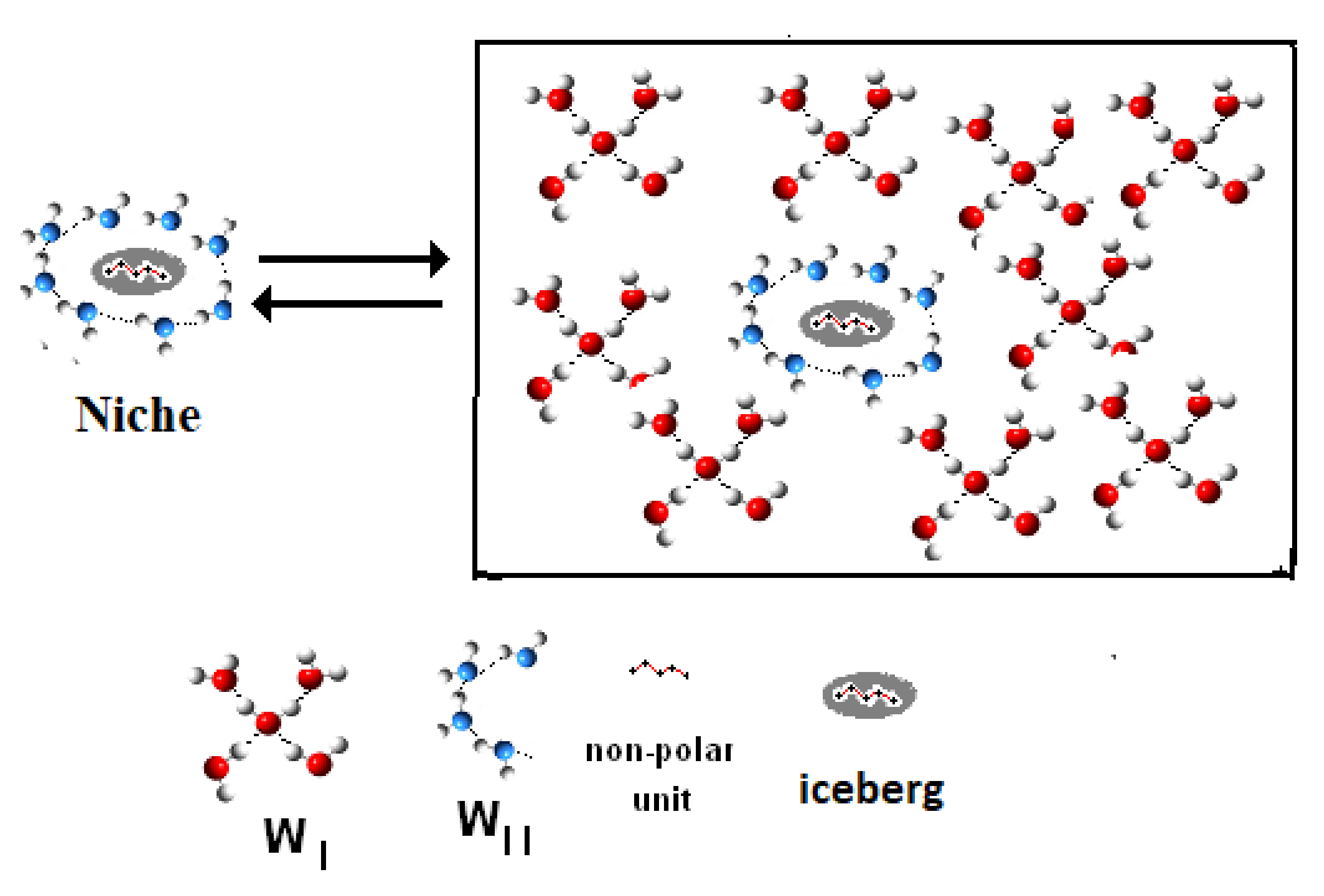
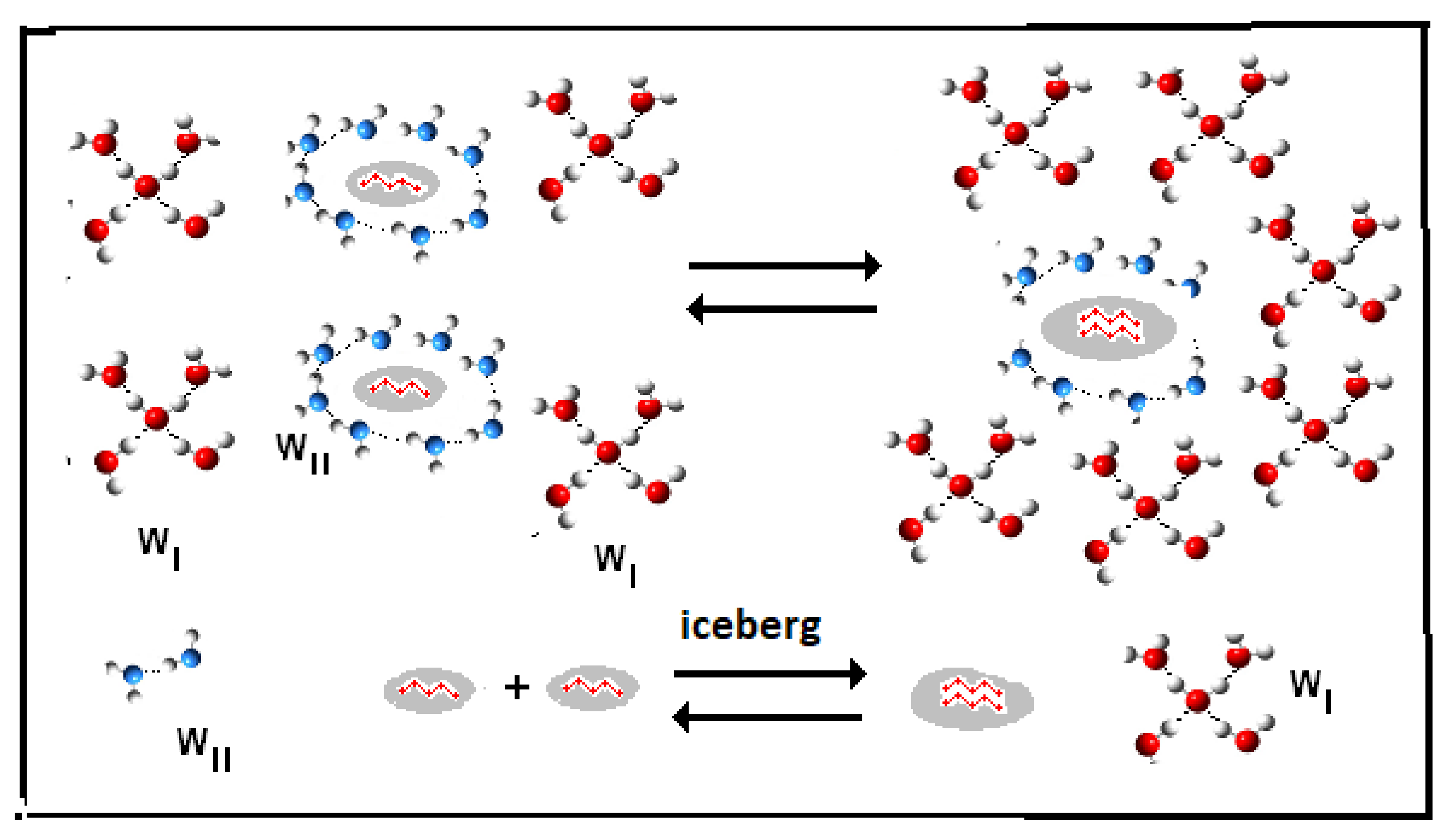
(Reaction A {–ξw WI (solvent) → ξw WII (iceberg, solute)}).
(b)
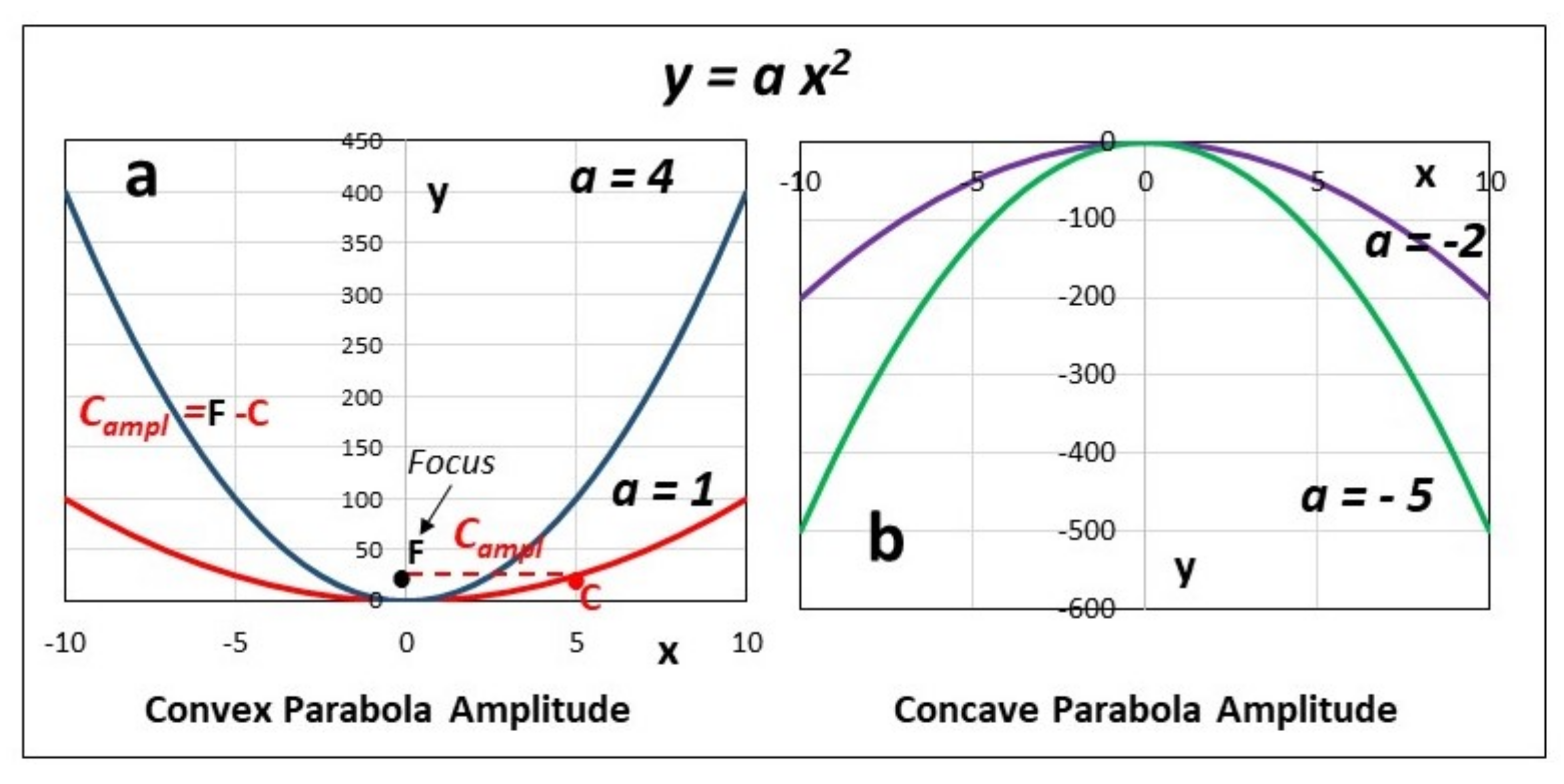
Convexity (ΔCp,hydr = ξw Cp,w > 0).
(c)
Iceberg size and water stoichiometry: ξw.
The same information elements are confirmed by the secondary function g(lnT) of the convoluted binding function RTlndual = {f(T) g(lnT)}.
In Class B, where we obtain the reaction of iceberg reduction (Figure 7), we obtain the information elements
(a)
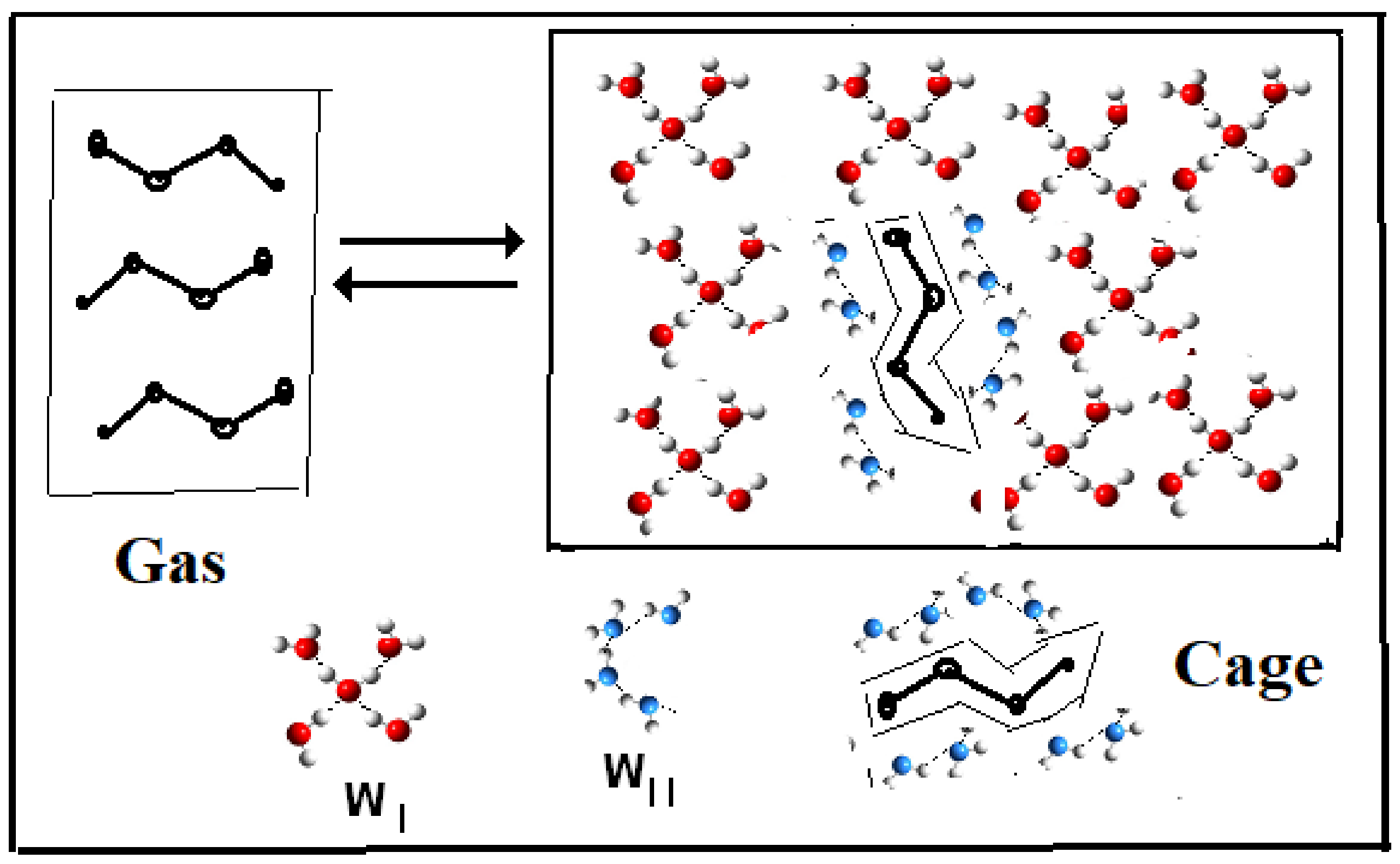
(reaction: B {–ξw WII (iceberg, solute)} → ξw WI (solvent).
(b)
Concavity (ΔCp,hydr = ξw Cp,w < 0).
(c)
Iceberg size and water stoichiometry: ξw.
Figure 7. Class B. Iceberg coalescing, with iceberg reduction.
Thermo 01 00022 g007
From the coincidence of the value of entropy at zero iceberg ΔS0(ξw = 0) = –86.4J K−1 mol−1, (see reference [5]) with the Trouton constant ΔHeb/Teb = ΔSevap = +86.9 ± 1.4 J K−1 mol−1, we can infer that the passage of gas molecules from the free state (Figure 8) to the trapping into the solvent implies a change in entropy (as change in kinetic energy) that is exactly the opposite of that for the passage from liquid state to vapor state (i.e., configuration entropy change for the condensation of gas is equal to the opposite of evaporation, –ΔSevap).

8. Structures of Thermodynamic Functions

At the end of the analysis of the structure of the thermodynamic functions of hydrophobic hydration processes, we can conclude:
(1)
The simulated free energy functions RlnKsimul, as calculated by any simulation functions, either FEP, or TI, MV, MC, etc., and applied to hydrophobic hydration processes are inadequate to represent the properties of biphasic systems with implicit solvent. Many important thermodynamic functions are ignored by these calculations and all the important information elements carried by these functions are completely lost.
(2)
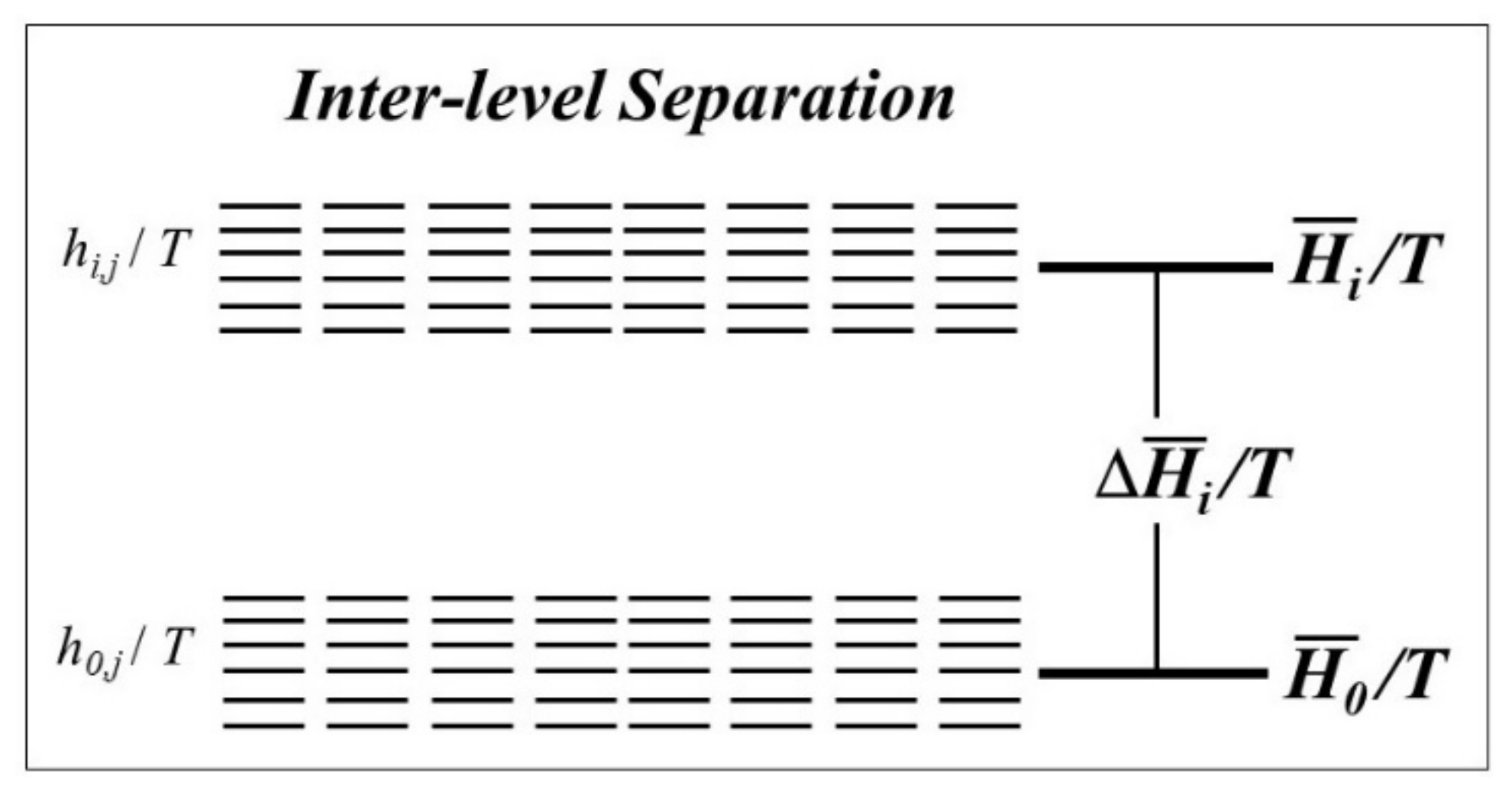
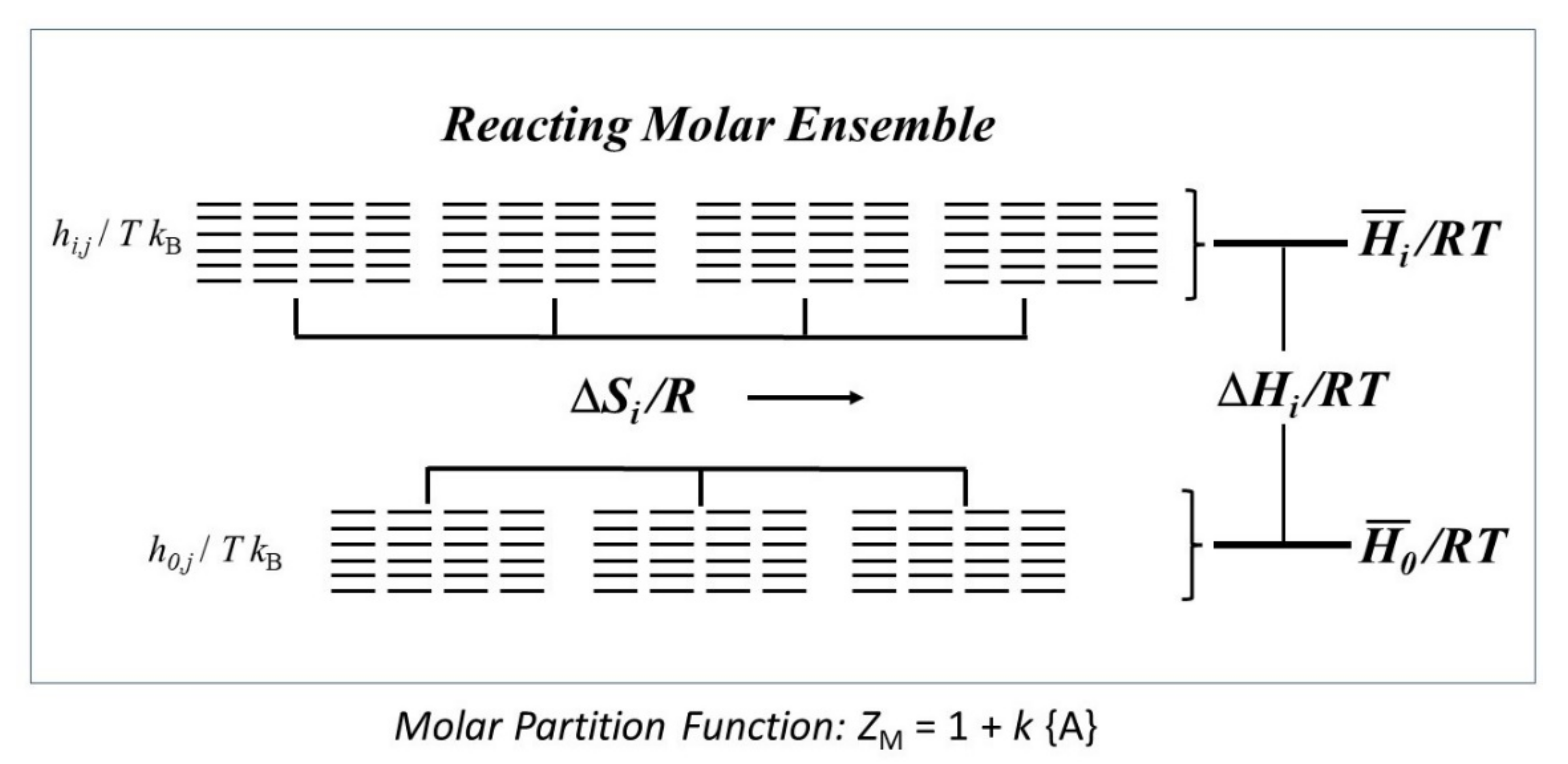
The hydrophobic hydration systems have a biphasic composition, constituted by a “non-reacting” molecule ensemble, at constant potential formed by the solvent and by a “reacting” mole ensemble formed by diluted solutes. The distribution of molecules over the sublevels hi,j of each macrolevel Hi follows a Boltzmann distribution, whereas the distribution of moles of reactants over macrolevels Hi follows a binomial distribution. The Ergodic Algorithmic Model (EAM) is adequate to the biphasic composition of aqueous solutions and suited to evaluate correctly the many essential information elements.
The thermodynamic potential of each hydrophobic hydration process can be experimentally determined at different temperatures and processed by the Ergodic Algorithmic Model (EAM), obtaining convoluted binding functions (a) RlnKapp = {f(1/Tg(T)} and (b) RTlnKapp = {f(Tg(lnT)} as developed from a dual-structure partition function {DS-PF} = {M-PF} · {T-PF}, where the thermal partition function {T-PF} is the thermal partition function of implicit solvent.
The statistical analysis of the unitary (for ξ = ±1) functions, which resulted to be constant in a statistically significant population of data, calculated by processing the curved binding functions, shows how the distribution of errors as a normal population validates the Ergodic Algorithmic Model (EAM) as the correct dual-structure model for the description of the thermodynamic properties of hydrophobic hydration processes. The statistical validation of the EAM model, discussed in ref. [8], is also reported in Appendix B. Another experimental method suited to the determinations of the information elements of a thermodynamic system in aqueous solution is calorimetry. Freire [27,28] showed how high affinity and selectivity, two essential properties of drugs, can be achieved by the optimization of enthalpic and entropic contributions to binding (the so-called “Thermodynamic Signatures”). If the calorimetric binding experiments are performed at a different temperature, the complete set of information elements can be obtained by applying the EAM model. This information is, therefore, essential not only from a speculative point of view, but also for application purposes, such as, for instance, lead optimization.
In any case, the statistical inference of Appendix B shows how the Ergodic Algorithmic Model (EAM) has a universal validity for every hydrophobic hydration process [8] and every hydrophobic hydration process must present the same behaviour. The functions required by the EAM must necessarily exist, for statistical inference. The first step is the search for an equilibrium constant or any appropriate potential function which is variable with temperature. The next step consists of a verification that the system presents the necessary ergodic properties. With these elements, one can determine the convoluted binding functions and then build up the EAM model.

9. Conclusions

The use of the Ergodic Algorithmic Model (EAM) with water as implicit solvent at constant thermodynamic potential μs, to calculate the thermodynamic properties of hydrophobic hydration systems, is highly recommended, instead of computer simulations with explicit solvent, the evaluation of only binding affinity not being enough either from a speculative or practical point of view. Every hydrophobic hydration process necessarily has the properties of an ergodic model, statistically validated. For a correct thermodynamic analysis of any hydrophobic hydration process in chemical, biochemical, and biological systems, these properties must be searched for.

Author Contributions

Conceptualization, E.F. and A.B.; formal analysis, E.F., C.C., and A.B.; supervision, A.B.; writing—original draft, E.F., C.C., and A.B. All authors have read and agreed to the published version of the manuscript.

Funding

This research received no external funding.

Data Availability Statement

The data processed are available in the specified references.

Acknowledgments

This work is dedicated to the memory of Professor Gian Paolo Chiusoli, Emeritus, University of Parma, who since 2009 had highly appreciated this EAM model as a landmark in the study of hydrophobic hydration processes.

Conflicts of Interest

The authors declare no conflict of interest.

Appendix A

Table A1. Ergodic Algorithmic Model (EAM, see ref. [9]).
Probability Space
Dual-Structure Partition Function (for Biphasic Systems)
{DS-PF} = {T-PF} · {M-PF}w}} = Kmot·1
{M-PF} = exp(ΔSmot/R), {T-PF} = exp(−ΔHmot/RT), exp(−ΔGmot/RT) = Kmot
exp(−ΔHmot/RT) exp(ΔSmot/R) = exp(−ΔGmot/RT) = Kdual
exp(Sdens/R) = aA−1 = xA−1 Φ−1 = xA−1· TCp,A/R
exp(Sint/Cp,A) = T
Kdual = Kmot · ζth
ζth = 1 (Implicit Solvent, at constant Thermodynamic Potential μs)
{M-PF} = Kmot → (Solute, Density Entropy parameter)
{T-PF} = ζth = 1 → (Solute, Intensity Entropy parameter)
aA = xA · Φ (aA = activity of A, Φ = T−Cp,A/R: Lambert thermal factor)
Ergodicity → (Dilution → Temperature)
(1/xA) = did(A) → dilution thermal factor TCp,A/R = 1/Φ
Thermodynamic Space
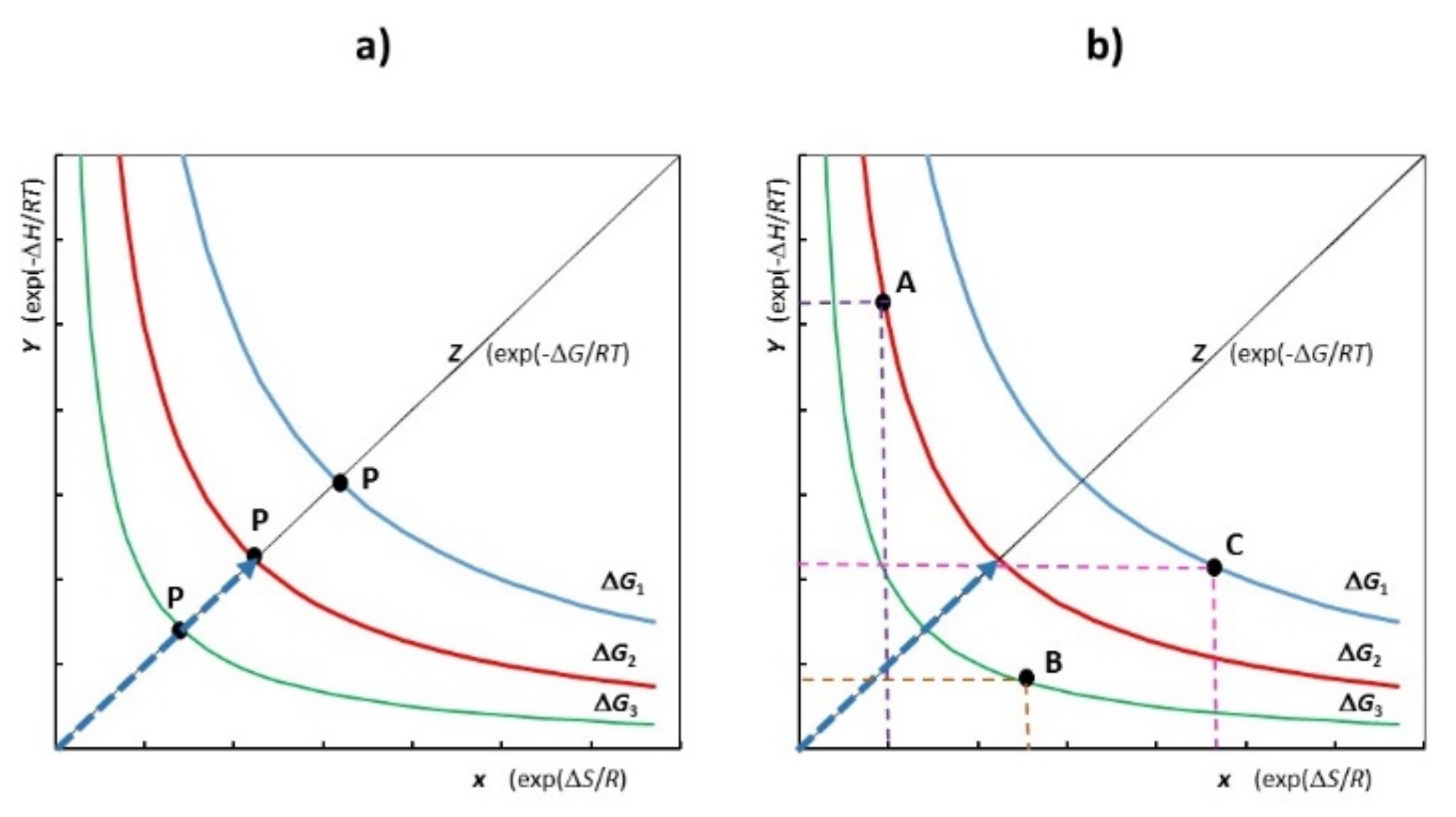
(A) Binding Function RlnKdual = (−ΔGdual/T) = {f(1/Tg(T)}
1.Curved convoluted function ({f(1/T)*g(T)})
Rln Kdual = {(−ΔHdual/T) + (ΔSdual)} = {(−ΔHmot/T) + (−ΔHth/T)} + {(ΔSmot) + (ΔSth)}
∂(RlnKdual)/∂(1/T) = −ΔHdual = −ΔHmot − ΔHth = −ΔHmot − ΔCp.hydrT (J mole−1)
2. Linear function (f(1/T))
RlnKmot = RlnKdual ={(−ΔHdual/T) + (ΔHth/T)} + {(ΔSdual) − (ΔSth)} = −ΔHmot/T + ΔSmot
∂(RlnKmot)/∂(1/T) = −ΔHmot (J mole−1)
(B) Binding Function RTlnKdual = (−ΔGdual) = {f(Tg(lnT)}
1.Curved convoluted function ({f(Tg(lnT)})
RTln Kdual = {−ΔHdual + T ΔSdual} = {−ΔHmot − ΔHth} + TSmot + ΔSth}
∂(RTlnKdual)/∂T = ΔSdual = ΔSmot + ΔSth = ΔSmot + ΔCp,hydrlnT (J K−1 mole−1)
2.linear function (f(T))
RTlnKmot = {−ΔHdual + ΔHth} + TSdual − ΔSth} = −ΔHmot + T ΔSmot
∂(RTlnKmot)/∂T = ΔSmot
(C) Activity: aA = f(xA,T)
dSDens = −Rdln aA = (−Rdln xA)T + (Cp,A dlnT)x
(D) Ergodicity
Density EntropyS/R) and Intensity Entropy (ΔH/RT)
(dSDens)T = (−Rdln xA)T = (Rdlndid,A)T → (Changing Density Entropy)
(dSInt)xA = (Cp,A dlnT)xA → (Changing Intensity Entropy)
TED (Thermal Equivalent Dilution)
(dSDen)T = (dSInt)xA
nw (Rdln did,A)T = nw (Cp,A dlnT) xA
(E) Hydrophobic Heat Capacity
ΔCp,hydr = ±ξw Cp,w; Cp,w = 75.36 J K1mol−1 (molar heat capacity for liquid water)

Appendix B

Table A2. Validation of the Ergodic Algorithmic Model (EAM). For analysis of unitary thermodynamic functions (*), see reference [8].
(a) Analysis within Classes
Class A:
iceberg formation
UnitRelative error
hfor>A= −22.7 ± 0.07kJ⋅mol−1 ξw−1±3.1%
sfor>A = −445 ± 3J⋅K−1⋅mol−1ξw−1±0.7%
Class B:
iceberg reduction
UnitRelative error
hred>B = +23.7 ± 0.6kJ⋅mol−1 ξw−1±2.51%
sred>B = +432 ± 4J⋅K−1⋅mol−1ξw−1±0.9%
(b) Comparison among Classes
EnthalpyEntropy
hfor>A = −22.7 ± 0.7 kJ mol−1 ξw−1sfor>A = −445 ± 3J K1 mol1 ξw−1
hred>B = +23.7 ± 0.6 Kj mol−1 ξw−1sred> B = +432 ± 4 J K1 mol1 ξw−1
mean abs.value <Δh>A,B = 22.95 ± 0.75mean abs.value <Δs>A,B = 438.5 ± 6.5
Student’s ratio: 0.75/0.92 = 0.815Student’s ratio: 6.5/5 = 1.3
(*) Mean values obtained from more than eighty different sets, with about 600 data points. Note the small variability ±σ, indicating that all the points belong to a unique homogeneous statistical population. Hypothesis: absolute values in Class A and B are equal: hypothesis accepted (mean in Class A = mean in Class B with sign reversed).

References

  1. Lambert, F.L. Configurational Entropy Revisited. J. Chem. Educ. 2007, 84, 1548–1550. [Google Scholar] [CrossRef]
  2. Lambert, F.L. The Misinterpretation of Entropy as “Disorder”. J. Chem. Educ. 2012, 89, 310. [Google Scholar] [CrossRef]
  3. Fisicaro, E.; Compari, C.; Braibanti, A. Entropy/enthalpy compensation: Hydrophobic effect, micelles and protein complexes. Phys. Chem. Chem. Phys. 2004, 6, 4156–4166. [Google Scholar] [CrossRef]
  4. Fisicaro, E.; Compari, C.; Duce, E.; Biemmi, M.; Peroni, M.; Braibanti, A. Thermodynamics of micelle formation in water, hydrophobic processes and surfactant self-assemblies. Phys. Chem. Chem. Phys. 2008, 10, 3903–3914. [Google Scholar] [CrossRef] [PubMed]
  5. Fisicaro, E.; Compari, C.; Braibanti, A. Hydrophobic hydration processes. General thermodynamic model by thermal equivalent dilution determinations. Biophys. Chem. 2010, 151, 119–138. [Google Scholar] [CrossRef] [PubMed]
  6. Fisicaro, E.; Compari, C.; Braibanti, A. Hydrophobic hydration processes. Biophys. Chem. 2011, 156, 51–67. [Google Scholar] [CrossRef] [PubMed]
  7. Fisicaro, E.; Compari, C.; Braibanti, A. Hydrophobic Hydration Processes. I: Dual-Structure Partition Function for Biphasic Aqueous Systems. ACS Omega 2018, 3, 15043–15065. [Google Scholar] [CrossRef] [PubMed]
  8. Fisicaro, E.; Compari, C.; Braibanti, A. Statistical Inference for Ergodic Algorithmic Model (EAM), Applied to Hydrophobic Hydration Processes. Entropy 2021, 23, 700–721. [Google Scholar] [CrossRef]
  9. Fisicaro, E.; Compari, C.; Braibanti, A. Intensity Entropy and Null Thermal Free Energy and Density Entropy and Motive Free Energy. ACS Omega 2019, 4, 19526–19547. [Google Scholar] [CrossRef]
  10. Chipot, C.; Pohorille, A. Free Energy Calculations. Theory and Application in Chemistry and Biology; Sperling: Berlin/Heidelberg, Germany, 2012. [Google Scholar]
  11. Pohorille, A.; Jarzynski, C.; Chipot, C. Good Practice in Free-Energy Calculation. J. Phys. Chem. B 2010, 114, 10235–10253. [Google Scholar] [CrossRef] [Green Version]
  12. Liu, P.; Dehez, F.; Cai, W.; Chipot, C. A Toolkit for the Analysis of Free-Energy Perturbation Calculations. J. Chem. Theory Comput. 2012, 8, 2606–2616. [Google Scholar] [CrossRef]
  13. Born, M. Volumes and heats of hydration of ions. Z. Phys. 1920, 1, 45–48. [Google Scholar] [CrossRef]
  14. Landau, L.D.; Lifshitz, E.M. Statistical Physics; ThriftBooks-Dallas: Seattle, WA, USA; The Claredon Press: Oxford, UK, 1938. [Google Scholar]
  15. Pearlman, D.A.; Charifson, P.S. Are Free Energy Calculations Useful in Practice? A Comparison with Rapid Scoring Functions for the p38 MAP Kinase Protein System. J. Med. Chem. 2001, 44, 3417–3423. [Google Scholar] [CrossRef]
  16. Zwanzig, R.W. High-temperature equation of state by a perturbation method. I. Nonpolar gases. J. Chem. Phys. 1954, 22, 1420–1426. [Google Scholar] [CrossRef]
  17. Chipot, C.; Rozanska, X.; Dixit, S.B. Can free energy calculations be fast and accurate at the same time? Binding of low-affinity, non-peptide inhibitors to the SH2 domain of the src protein. J. Comput.-Aided Mol. Des. 2005, 19, 765–770. [Google Scholar]
  18. Kirkwood, J.G. Statistical mechanics of fluid mixtures. J. Chem. Phys. 1935, 3, 300–313. [Google Scholar] [CrossRef]
  19. Chodera, J.D. Alchemical free energy methods for drug discovery: Progress and challenges. Curr. Opin. Struct. Biol. 2011, 21, 150–160. [Google Scholar] [CrossRef] [Green Version]
  20. Bennett, C.H. Efficient Estimation of Free Energy Differences from Monte Carlo Data. J. Comput. Phys. 1976, 22, 245–268. [Google Scholar] [CrossRef]
  21. Ferrenberg, A.M.; Swendsen, R.H. New Monte Carlo technique for studying phase transitions. Phys. Rev. Lett. 1988, 61, 2635–2638. [Google Scholar] [CrossRef] [Green Version]
  22. Jarzynski, C. Non equilibrium Equality for Free Energy Differences. Phys. Rev. Lett. 1997, 78, 2690. [Google Scholar] [CrossRef] [Green Version]
  23. Jarzynski, C. Equilibrium free-energy differences from nonequilibrium measurements: A master-equation approach. Phys. Rev. E 1997, 56, 5018–5035. [Google Scholar] [CrossRef] [Green Version]
  24. Abel, R.; Wang, L.; Harder, E.D.; Berne, B.J.; Friesner, R.A. Advancing Drug Discovery through Enhanced Free Energy Calculations. Acc. Chem. Res. 2017, 50, 1625–1632. [Google Scholar] [CrossRef]
  25. Knight, J.L.; Brooks, C.L., III. λ-dynamics free energy simulation methods. J. Comput. Chem. 2009, 30, 1692–1700. [Google Scholar] [CrossRef]
  26. Talhout, R.; Villa, A.; Mark, A.E.; Engberts, J.B.F.N. Understanding Binding Affinity: A Combined Isothermal Titration Calorimetry/Molecular Dynamics Study of the Binding of a Series of Hydrophobically Modified Benzamidinium Chloride Inhibitors to Trypsin. J. Am. Chem. Soc. 2003, 125, 10570–10579. [Google Scholar] [CrossRef]
  27. Freire, E. The binding thermodynamics of drug candidates. Methods Princ. Med. Chem. 2015, 65, 1–13. [Google Scholar]
  28. Schön, A.; Freire, E. Enthalpy screen of drug candidates. Anal. Biochem. 2016, 513, 1–6. [Google Scholar] [CrossRef] [Green Version]
Figure 1. Hyperbolic partition functions in probability space. (a) exp(−ΔΓ/T) = exp(−ΔG·(cos 45°)/RT); (b) exp(−ΔGA/RT) = exp(−ΔHA/RT) exp(ΔSA/R).
Thermo 01 00022 g001
Figure 2. Vector representation of free energy in thermodynamic space (a) RlnK = (ΔΓ/T)/cos 45° = (−ΔG/T); (b) RlnK = ΔG/T = ΔH/T + ΔS.
Thermo 01 00022 g002
Figure 3. The distribution of molecules over sublevels hi,j of each macrolevel Hi follows a statistical distribution: passage of molecules from population h0,j to population hi,j can be calculated by integration (HEP).
Thermo 01 00022 g003
Figure 4. The distribution of moles over each macrolevel Hi follows a binomial mathematical distribution, not calculated by integration. Now, we have two methods for calculating partition functions.
Thermo 01 00022 g004
Figure 5. (a) The convexity of the parabolic function depends on the positive coefficient (ΔCp,hydr > 0); (b) The concavity of the parabolic function depends on the negative coefficient (ΔCp,hydr < 0).
Thermo 01 00022 g005
Figure 6. Class A. Reaction of iceberg formation.
Thermo 01 00022 g006
Figure 8. Change in kinetic thermal energy (entropy change) for gas trapping in a cage and for passage of vapor to liquid (condensation).
Thermo 01 00022 g008
Table 1. Information elements from EAM.
∂(RlnKmot)/∂(1/T) = −ΔH°mot (J mol−1)
∂(RTlnKmot)/∂T = ΔS°mot (J K−1 mol−1)
ΔCp,hydr = ±ξw Cp,w
with Cp,w = 75.36 J·K−1mol−1 (molar heat capacity for liquid water)
ΔCp,hydr = +ξw Cp,w (Class A, convex binding function)
ΔCp,hydr = −ξw Cp,w (Class B, concave binding function)
Table 2. Convoluted binding functions. Motive functions.
ENTHALPYENTROPY
RlnKdual = −ΔG°/T = −ΔHdual/T + Sdual.
    = −{ΔHmot+ΔCp,hydr,T}/T + ΔS’
where
ΔCp,hydr = 2202(ΔHdual)/∂T
ΔC p,hydr = isobaric heat capacity(*)
RT lnKdual = −ΔG° = −ΔHdual + T ΔSdual
    = −ΔH’+TSmot + ΔCp,hydr lnT}
where
ΔCp,hyd = ∂(ΔSdual)∂lnT
ΔCp,hydr = isobaric heat capacity(*)
Motive Function
from primary function f(1/T) in
RlnKapp = {f((1/T)*g(T)}
Motive Function
from primary function f(T) in
RTlnKapp = {f((T)*g(lnT)}
R lnKmot = −(ΔHmot/T) + ΔSRT lnKmot = −ΔHmot +T ΔS°
(*) ΔCp,hydr numerically equal for enthalpy and entropy: the same constant curvature amplitude (mathematical constraint), the same molecular event, i.e., the same passage of state of water (chemical constraint).
Publisher’s Note: MDPI stays neutral with regard to jurisdictional claims in published maps and institutional affiliations.

