Metaheuristic Optimized Random Forest Regression with Streamlit Web Application for Predicting Jute Yarn Tenacity

Abstract

Yarn tenacity is one of the vital quality parameters that determine the performance, fabric durability and end use suitability. The tenacity of yarn is largely influenced by the fibre characteristics used. The physical properties of jute fibres, including root content, defect, bundle strength, and fineness, exert a significant influence on yarn tenacity. This study utilized metaheuristic optimized random forest regression (RFR) to predict jute yarn tenacity from fibre parameters. The hyperparameters of the RFR models were optimized using four metaheuristic algorithms: whale optimization algorithm (WOA), grey wolf optimization (GWO), beetle antennae search (BAS) and ant colony optimization (ACO). The model utilized a dataset comprising 414 experimental data with 70% data for training and 30% for testing the model, using input variables such as bundle strength (g/tex), defects (%), root content (%) and fineness (tex) to predict yarn tenacity (cN/tex). The developed models effectively predicted yarn tenacity. However, RFR–GWO achieved slightly better performance with R² of 1.0 for training set and 0.96 for test set. Regarding execution time, RFR–GWO is the fastest requiring only 14.25 s. SHAP analysis revealed that bundle strength and root content of jute fibre are the most influential factors, whereas defect and fineness exert the least influence on model’s prediction. The best model RFR–GWO was deployed into an interactive Streamlit web application, offering an intuitive and user-friendly platform for the real-time estimation of yarn tenacity.

1. Introduction

Jute, often referred to as golden fibre, is one of the most important cash crops of the north-eastern part of India and Bangladesh. It is cultivated mainly for extraction of bast fibre, which is considered as the most economical and extensively used industrial bast fibre [1]. Owing to its biodegradability, renewability and moderate mechanical properties, jute fibre has gained widespread acceptance as an alternative to synthetic fibres [2]. The extracted fibre has been extensively used in the manufacture of ropes, sacks, carpets, bags and furnishing materials. With growing concern for the environment and global demand for sustainable alternative to synthetic fibres, the demands for jute fibre-based textiles have increased.

Yarn, the primary component of textiles, plays a crucial role in determining the performance, appearance, and durability of the end products. Among the various properties, yarn tenacity is one of the vital quality parameters, impacting not only the final product but also determining the yarn’s ability to withstand mechanical stresses during processes such as winding, weaving, knitting and subsequent fabric finishing [3]. The tenacity of the yarn is affected by various factors viz., fibre properties, spinning technique and process parameters [4]. Among these, fibre properties have the major effect on yarn tenacity. The physical properties of jute fibre like root content, defect, bundle strength and fineness were also reported to affect the yarn tenacity and other properties [5,6].

Given the significant influence of yarn on the overall quality of the finished products, accurate prediction of yarn tenacity is very crucial. Accurate prediction of yarn tenacity prior to production helps reduce process cost and material waste and assists in selecting suitable fibre and process optimizations to obtain the desired yarn tenacity [7]. Traditionally, experiential, statistical and mathematical models are used to foretell yarn strength from jute fibre properties. Bandyopadhyay [8] developed regression equations to predict jute yarn strength based on the tenacity and fineness of jute fibres. Apart from jute fibre tenacity and fineness, parameters such as root content and defect also have a significant influence on yarn tenacity, yet no previous work has so far reported their influence. Given that regression models do not consistently predict experimental values accurately, exploring alternative prediction methods is necessary.

In recent years, machine learning (ML) has evolved as a potent computational tool across various scientific fields, including textiles, with the potential to overcome the shortcomings of conventional modelling techniques. Machine learning has the ability to uncover relationships in large, high dimensional datasets without prior assumptions, handling multiple influencing parameters and enhancing predictive accuracy. ML has been widely applied in the textile industry for investigating fibre properties [9], yarn [10,11], and the fabric properties of natural fibres [12,13]. Considerable progress has been made in the application of machine learning techniques for predicting yarn properties, especially cotton [4,11,14], polyester [15,16] and cotton/polyester blends. However, no study has specifically focused on jute yarn properties. Furthermore, there are no reports of research on the influence of jute fibre properties such as root content, bundle strength, fineness, and defects on yarn tenacity.

Most machine learning models developed for predicting the yarn strength of cotton, polyester, and cotton-blend yarns are based on artificial neural networks (ANNs). Although ANNs are regarded as universal function approximators capable of learning complex relationships from data, they largely operate as black-box models and do not explicitly reveal the relationships between input variables and output responses. Consequently, some studies have explored alternative approaches, such as fuzzy logic [11] and tree-based regression models [4]. Unlike ANN models, tree-based methods such as random forest offer better interpretability and enable users to gain clearer insights into the relationships between input parameters and output parameter [17]. Furthermore, it efficiently handles large datasets, manages numerous input variables without omitting any, identifies the most influential factors in the model, and captures nonlinear relationships between the input variables.

The major bottleneck that hinders the predictive performance of the standard ML models is the hyperparameters optimization [18]. To overcome the aforementioned limitation, metaheuristic algorithms have been incorporated into conventional ML models [19]. Zhang et al. [20] employed an artificial neural network (ANN) with particle swarm optimization (PSO) to forecast yarn strength. The results indicated that the hybrid approach enhanced the prediction accuracy. Song and Fan [21] integrated a generalized regression network (GRNN) with metaheuristic optimization i.e., Harris hawk optimization, for foretelling yarn hairiness. The experimental results reveal that the hybrid model achieved remarkably high accuracy in predicting yarn hairiness. Hu et al. [22] developed a hybrid deep belief network (DBN)–particle swarm optimization (PSO) algorithm to predict yarn quality. The study revealed that the hybrid approach produced a higher R² value compared to the standalone DBN model. These studies demonstrated that metaheuristic algorithms provide an efficient and systematic framework for exploring the hyperparameters of machine learning models, thereby significantly improving their predictive accuracy.

ML implementations often demand programming expertise, which can be a barrier for non-technical users, as mistakes in input or parameter adjustments may result in inaccurate predictions. Integrating machine learning with a web application is vital to make predictive models accessible and usable by end-users who may not have programming expertise [9]. A web interface allows users to input data, run predictions, and visualize results in real time, enhancing the practical applicability of the model. It also facilitates faster experimentation with different input scenarios, improves user experience, and ensures wider deployment across devices and platforms. Without such integration, the usability of machine learning models remains limited to developers and data scientists.

The primary objective of the study is to develop metaheuristic algorithms-optimized RFR for accurate prediction of jute yarn tenacity from jute fibre parameters. To achieve this, four metaheuristic algorithms, WOA, GWO, BAS and ACO, were used to tune hyperparameters of RFR. Furthermore, this study developed web application for the deployment of best model.

2. Materials and Methods

2.1. Experiment and Data Collection

In the present study, jute fibres (Corchorus olitorius L.) collected from farmers’ fields across India were used. Fibre qualities such as bundle strength, root content, defects and fineness were evaluated following the IS: 271 (2020) standard [5], with standard laboratory conditions of relative humidity and temperature of 65 ± 2% and 27 ± 2 °C, respectively. Root content refers to the hard, barky portion present at the basal end of the reed. Bundle strength denotes the capacity of a fibre bundle, standardized by weight in instrumental testing, to withstand deformation or breakage when subjected to applied forces. Fineness represents the fibre’s diameter, linear density, or a combination of both. Defects arise mainly from improper processing and include specky fibres caused by inadequate washing, croppy fibres with uneven or coarse tips, rooty and dazed fibres, hunka characterized by woody or bark fragments, as well as weak, dead, sticky, knotty, or mossy fibres resulting from excessive retting. Bundle strength was determined with a digital bundle strength tester (Manufacture: Deep Micro system, Kolkata, India, Model No: NINFET-AEFBST-MF01), fineness was assessed with a digital fineness metre (Manufacture: Deep Micro system, Kolkata India, Model No: NINFET-DFM-MF01) [23], root content was measured on a length basis and defects were calculated on a weight basis.

2.1.1. Processing of Jute Fibre

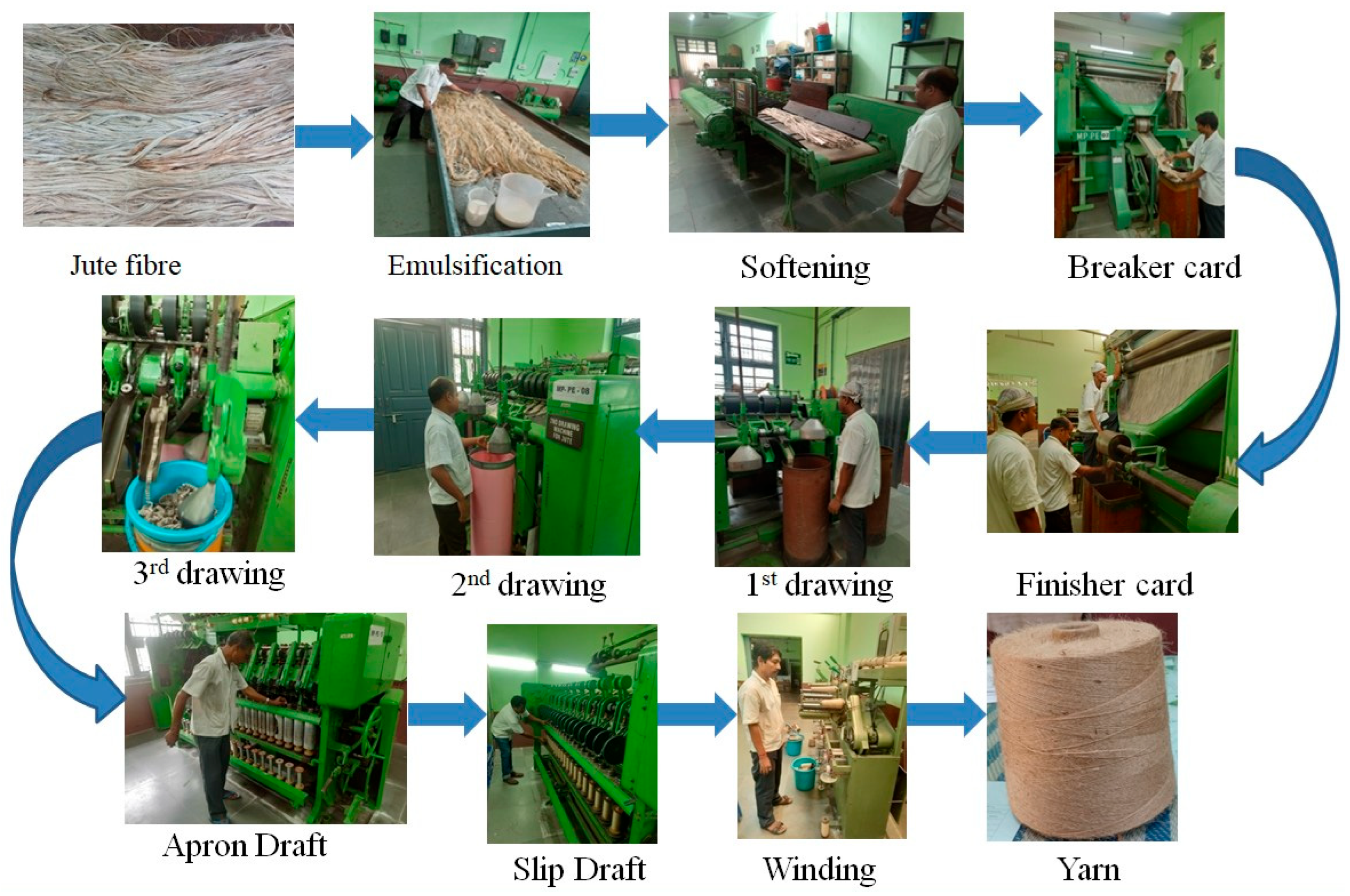
The yarn production process is shown in Figure 1. After grading of jute fibre, samples were conditioned with 35% emulsion (jute batching oil and water) and softened, using a softener machine (Manufacture: Douglas Fraser and sons, Arbroath, Scotland). Thereafter the fibres were kept in a closed container for 48 h for proper dissipation of moisture throughout the surface to core of the fibres. After 48 h, the fibres were taken out and passed through a 2-stage carding process (breaker card and finisher card) for proper fibrillation and opening to produce slivers. Finisher card slivers were then processed through a 3-stage drawing process for making the fibres parallel and drafted (3.7, 5.5 and 8.5 draft at the 1st, 2nd and 3rd drawing machine, respectively) and followed by spinning in an apron draft machine. The settings of the spinning machine (draft and twist change pinion) were adjusted as per the requirements of yarn linear density and twist. The specifications of the processing machines and their operational parameters are presented in

Table 1. Specifications of the processing machines.

Sl. No.	Particulars	Specifications
1	Softener Machine	Type—FD 31, Serial—189 No. of rollers: 24 pair
2	Breaker Card	Type—JF2, Serial—C1503 3 ½ pair, Half circular
3	Finisher Card	Type—JF4, Serial—C5040 3 ½ pair, Half circular
4	First Drawing Machine	Type—Screw Gill, Serial—004
5	Second Drawing Machine	Type—Screw Gill, Serial—009
6	Third Drawing Machine	Type—Screw Gill, Serial—FP24823
7	Spinning Machine	Type—Slip Draft, Serial—3/64 No. of Spindles: 20
8	Spinning Machine	Type—Apron Draft, Serial—36003 No. of Spindles: 20

and

Table 2. Operational parameters of different processing machines.

Carding Machines
Name of the Machine	Draft	Doubling	Max. Delivery Speed (m/min)	Nominal Sliver Weight (Ktex)
Breaker Card (JF2)	10–25	-	64	110
Finisher Card (JF4)	10–20	11–12	68	80
1st Drawing	4.37	2	22	40
2nd Drawing	5.5	3	25	20
3rd Drawing	8.5	2 or 3	50	7
Spinning Machines
Name of Machine	Draft	Maximum Spindle RPM	Max. Delivery Speed (m/min)	Nominal Yarn Count (tex)
Slip Draft	10–22	3800	22	275–550
Apron Draft	10–29	4250	26	3–7 Lb/spindle yarn

.

2.1.2. Testing of Jute Yarn

The yarn tenacity was measured in accordance with IS 1670 [24] using a Universal Testing Machine (Instron, Model 5967) equipped with a 500 N load cell. Prior to testing, the yarn samples were conditioned and tested under standard laboratory conditions (Relative humidity: 65 ± 2%, Temperature: 27 ± 2°C). The samples were tested using a gauge length of 610 mm and a pretension of 0.5 cN/tex.

2.1.3. Data Set Splitting

A dataset containing 414 valid input and output variables were gathered from the experiments. The dataset was randomly divided into training and testing with a 70:30 proportion. Consequently, 290 samples were allocated for training the model and 124 samples were reserved for testing to validate the model’s accuracy and generalization capacity.

2.2. Random Forest Regression

The random forest regressor is one of the effective and widely employed data analysis tools. This robust machine learning technique allows for the analysis of complex dataset and makes accurate predictions. During training, random forest employed for regression, generates a large number of trees and the final result is obtained by averaging the predictions from all those trees. Random forests (RFs) address the problem of decision trees overfitting to their training data. Breiman [25] developed an enhanced version of original random forest algorithm with a combination of randomness feature selection and bagging techniques. Each bootstrap sample (Db) is created from taking n samples from the original data D, containing N examples. Replacement of examples permitted during the sampling process. Typically, the bootstrap data set covers about two-thirds of the original data and excludes repeated examples. Using the input vector x, the bootstrap subsets serve as the basis for constructing K independent regression trees. In regression tasks, the final prediction of the random forest is obtained by averaging the outputs of the K regression trees.

$$\mathrm{RFR} \mathrm{Prediction}={\displaystyle \frac{1}{k}}\sum _{k=1}^k{h}_k\left(x\right)$$

(1)

The bagging technique primarily reduces the decision trees’ variance without significantly affecting its bias. During bagging, the samples left out from the training k regression trees are combined to generate the out-of-bag dataset. Using the out-of-bag dataset, the performance of the k^th regression tree is evaluated by calculating the mean square error.

$$\mathrm{M}\mathrm{S}\mathrm{E}={\displaystyle \frac{1}{n}}\sum _{i=i}^n{(y_i-m_{iOOB})}^2$$

(2)

where Y_i is the i^th prediction; M_i is the mean of i^th prediction from all the trees.

2.3. Metaheuristic Algorithms

Metaheuristic algorithms are advanced optimization approaches inspired by natural processes, developed to efficiently address complex, nonlinear and multi-objective problems where traditional deterministic or gradient-based techniques are ineffective. In the present study, four metaheuristic algorithms such as WOA, GWO, BAS and ACO are selected due to their capability to optimize the hyper parameters of the models.

2.3.1. Whale Optimization Algorithm (WOA)

Mirjalili and Lewis [26] introduced the whale optimization algorithm, drawing inspiration from the collective behaviours of humpback whales. The hunting strategy of these whales mainly involves three actions: encircling their prey, performing spiral bubble-net attacks, and searching for potential targets.

Encircling Prey

In this algorithm, whales function as search agents, and their respective positions determine the potential solutions they represent in the optimization process. The prey position represents the best solution and once this optimal solution is identified, the whales update their positions accordingly. This behaviour can be described using the following equations

$$D_{i,j}^L=\left|c·{pbest}_j-p_{i,j}(t)\right|$$

(3)

$$p_{i, j}\left(t+1\right)={pbest}_j-{a·D}_{i, j}^L$$

(4)

where t is the current iteration; p_i,_j is the position of i^th whale in the jth dimension; pbest is the current best position of prey. It is worth mentioning here that pbest should be updated when a better solution is found; a and c are coefficients.

The vectors a and c are calculated as follows

$$a=2 \left(2r-1\right)\left(1-{\displaystyle \frac{t}{tmax}}\right)$$

(5)

$$c=2r$$

where r is a random number [0, 1] and tmax is the maximum iterations

As iterations proceed, the value of the parameter a steadily decreases toward zero, which effectively regulates the shrinking encircling movement of the whales around the prey.

Bubble-net attacking

Alongside the shrinking encircling mechanism, the whales also update their positions by following a spiral path during the exploitation phase of the whale optimization algorithm. This behaviour is represented by the following equation

$${ p}_{i, j}\left(t+1\right)=e^{bl}·\cos \left(2\Pi l\right)· p_{i, j}^{\prime }+{pbest}_j$$

(6)

where $p_{i, j}^{\prime }=\left|{pbest}_j-p_{i, j}\left(t\right)\right|$ indicates the distance between the ith whale and the prey in the jth dimension; b is constant and l is a random number [−1, 1].

During the hunting process, the whale swims in a spiral pattern while simultaneously contracting the encircling radius. To simulate this behaviour in the whale optimization algorithm, a 50% probability threshold is established to decide the approach for updating the whales’ positions. The corresponding mathematical formula is described below

$$p_{i, j}\left(t+1\right)=\left\{\begin{array}{c}{pbest}_j-a·D_{i, j }^L r<0.5\\ e^{bl}·\cos \left(2\Pi l\right)· D_{i, j}^L+{pbest}_{j } r\ge 0.5 \end{array}\right.$$

(7)

Search for prey

During exploration phase of WOA, the whales search randomly based on their positions relative to one another. Additionally, the algorithm uses the absolute value of the parameter a to determine whether to enter the exploration or exploitation stage. Specifically, exploration is performed when $\left|a\right|>1$ and the WOA to perform a global search. The mathematical model is described below.

$$D_{i, j}^R=\left|c·{prand}_j\left(t\right)-p_{i, j}(t)\right|$$

(8)

$$p_{i, j}\left(t+1\right)={prand}_j\left(t\right)-a·D_{i, j}^R$$

(9)

where ${prand}_j\left(t\right)$ is a position of whale randomly selected from the current population.

2.3.2. Grey Wolf Optimizer (GWO)

Mirjalili et al. [27] introduced grey wolf optimization, which emulates the hunting behaviour and leadership hierarchy of grey wolves found in nature. Grey wolves belong to canidae family, live in packs and have a strict social dominant discipline. Based on their roles within the pack, grey wolves are classified into four groups: alpha, beta, delta, and omega. The predation process of grey wolf pack can be divided into three stages viz., encircling, hunting and attacking.

Encircling

After determining the location of prey, grey wolves begin to encircle it.

$$D_p=\left|C·x_p\left(t\right)-x(t)\right|$$

(10)

$$x\left(t+1\right)=x_p\left(t\right)-A·D_p$$

(11)

where x(t) is one grey wolf, t is the number of iteration, and x_p(t) specifically refers to α, β, δ; x(t+1) is next position it arrives; A and C are coefficient vectors

A and C are determined by

$$A=2a{r}_1-a$$

(12)

$$C=2r_2$$

where r₁ and r₂ are random vectors [0, 1]; a is a decreasing value [0, 2]

Hunting

Following the encircling its prey, the grey wolves—led by the alpha, beta, and delta—begin the hunting process. The following mathematical expressions provide this fact;

$$\left\{\begin{array}{c}{D}_{\alpha }=\left|C_1{X}_{\alpha }-X\left(t\right)\right|\\ D_{\beta }=\left|C_2{X}_{\beta }-X\left(t\right)\right|\\ D_{\delta }=\left|C_3{X}_{\delta }-X\left(t\right)\right|\end{array}\right.$$

(13)

$$\left\{\begin{array}{c}{X}_1=\left|X_{\alpha }\left(t\right)-A{D}_{\alpha }\right|\\ X_2=\left|X_{\beta }\left(t\right)-A{D}_{\beta }\right|\\ X_3=\left|X_{\delta }\left(t\right)-A{D}_{\delta }\right|\end{array}\right.$$

(14)

$$X_{p }\left(t+1\right)={\displaystyle \frac{X_1+X_2+X_{13}}{3}}$$

(15)

Attacking

The grey wolves encircle their target and start organizing the attack to capture it. When the value of $\left|A\right|\ge 1$, wolves keep a certain distance from the prey, enabling a global search. Conversely, when $\left|A\right|<1$, the grey wolf pack gradually approaches the prey and eventually completing the hunt.

2.3.3. Beetle Antennae Search Algorithm (BAS)

Jiang and Li [28] proposed beetle antennae search algorithm, which emulates the foraging behaviour of beetles using their antennae to detect odour source, representing optimal solutions in the search space. The beetle moves to the left if its left antenna detects a stronger scent of food; otherwise, it moves to the right.

Position of antennae

The position of left and right antennae of beetles can be expressed as below

$$\left\{\begin{array}{c}{P}_r=P+c·d \\ P_l=P-c·d\end{array}\right.$$

(16)

where p represents the current position of the beetle; c denotes the distance between the centre of mass of the beetle and the antennae; d denotes the random unit vector.

$$d={\displaystyle \frac{rand (D, 1)}{‖rand (D, 1)‖}}$$

(17)

Next Position of Beetle

To model how the beetle decides its direction based on the difference in odour concentration detected by its antennae, a specific mathematical expression is employed

$$P^{t+1}=P^t+{\delta }^t\times r_d\times sign (f\left(P_r\right)-f\left(P_l\right))$$

(18)

$$sign (P)=\left\{\begin{array}{c}1, P>0\\ 0, P=0\\ -1, P<0 \end{array}\right.$$

where δ^t is the step size of the beetle at time t, f(P_r) and f(P_l) indicates fitness function.

2.3.4. Ant Colony Optimization (ACO)

Ant colony optimization (ACO) is inspired by the natural foraging behaviour of ants. In nature ants find the shortest paths route between their nest and food sources by depositing chemical substances called pheromones, which guide other ants toward efficient path. When an ant locates food, it returns to the colony while leaving a pheromone along the path. Subsequent ants are more likely to follow paths with stronger pheromone concentrations. Through this collective behaviour of trail reinforcement and exploration, the ant colony gradually converges on the most efficient or shortest route connecting the nest and the food source.

Transition rule

The transition rule defines the probabilistic strategy by which an ant selects its next node (or state) during the process of solution construction.

Mathematically, the probability $p_{ij}^k(t)$ that ant k moves from node i to node j at iteration t is given by

$$P_{ij}^k(t)={\displaystyle \frac{{[T_{ij} (t)]}^{\alpha }· {\left[n_{ij}\right]}^{\beta }}{{\sum }_{l\in N_i^k}{[T_{il} (t\left)\right]}^{\alpha }· {\left[n_{il}\right]}^{\beta }}}$$

(19)

where T_ij(t) is the pheromone intensity on edge i→j at time t; n_ij is heuristic information; α regulates influence of pheromone; β regulates the influence of heuristic information; N_i^k is the feasible neighbours of node i for ant k.

Pheromone update

After completing all iterations for all ants, the pheromone update rule is applied to adjust the pheromone concentration along the paths traversed by the ants. The updated pheromone concentration is calculated using the following formula:

$$T_{ij}\left(t+1\right)=\left(1-\rho \right)T_{ij}\left(t\right)+\rho ∆T_{ij}\left(t\right)$$

(20)

where ρ is the pheromone volatile factor and $∆T_{ij}\left(t\right)$ indicates the increment of pheromone between node i and node j in this iteration process.

$$∆T_{ij}\left(t\right)=\left\{\begin{array}{c}{\displaystyle \frac{Q}{L^{k, }}}(i j\in L^k)\\ O\end{array}\right\}$$

where Q is the pheromone intensity, and L^k is the total distance of the k^th ant in the current iteration.

2.4. Metaheuristic Algorithms for Optimizing Random Forest Regressor

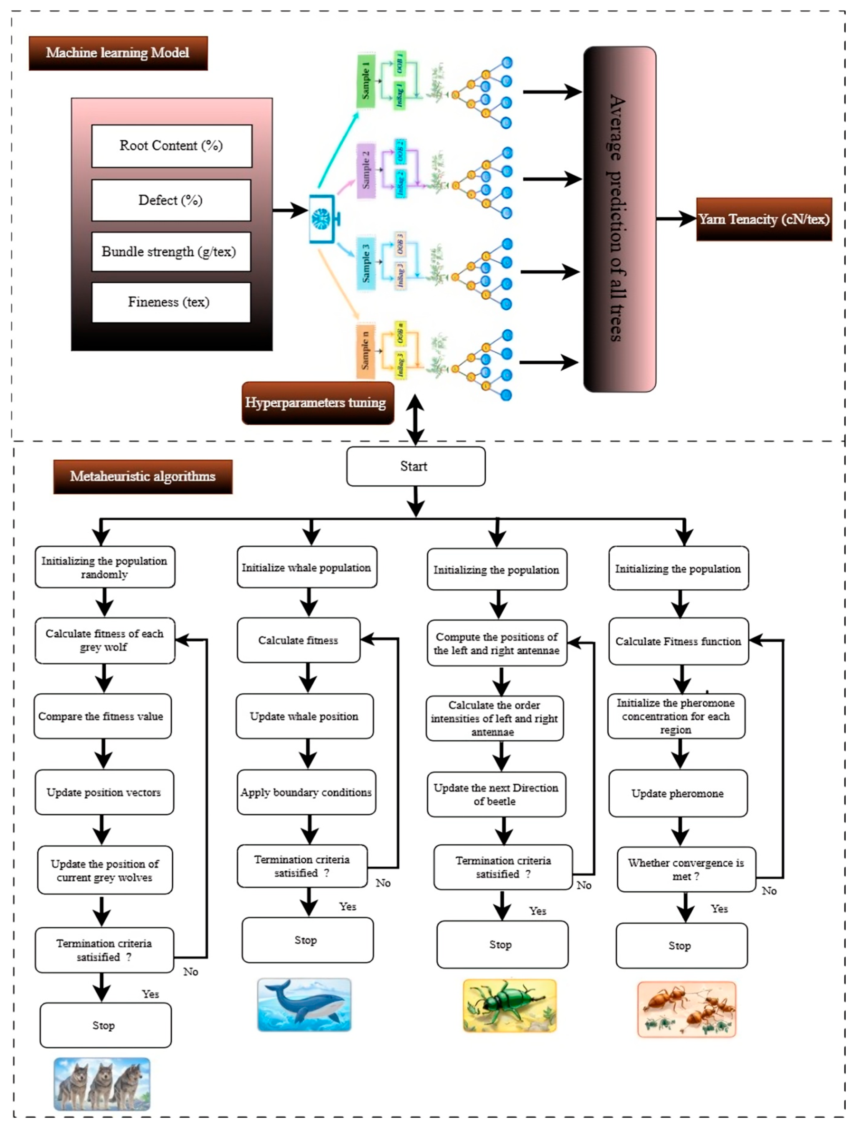
The optimization of hyperparameters is crucial for robust machine learning model performance. Unsuitable hyperparameters can lead to inaccurate results and suboptimal model performance. However, identifying the optimal hyperparameters through manual or statistical approaches remains a considerable challenge. In this study, four metaheuristic algorithms were used to optimize the hyperparameters of the random forest regressor. Figure 2 illustrates architectural flowchart of metaheuristic algorithm-optimized random forest regressors. The machine learning models were implemented using Python on Google Colab, a cloud-based Jupyter Notebook platform. Random forest regression was implemented using the Scikit-learn library. Among the total 414 data points, 70% were allocated for model training and the remaining 30% were retained to assess predictive accuracy.

The hyperparameters search space was defined as follows: n_estimators ranged from 50 to 300, max_depth varied between 2 and 20, min_samples_split was set between 2 and 10, and min_samples_leaf ranged from 1 to 5. Optimization of hyperparameters was conducted using metaheuristic algorithms, including GWO, WOA, ACO and BAS, which were custom developed using NumPy in the Google Colab environment. These metaheuristic approaches involve several distinct phases: initializing the population, evaluating fitness, and iteratively searching for the optimal solution.

Table 3. Parameters setting for meta-heuristic algorithms.

Sl. No.	Algorithm	Parameters Setting
1	GWO	n_wolves: 15 n_iterations: 25
2	BAS	Step size: 2.0 Dθ = 5.0 Decay: 0.9 n_iterations: 25
3	WOA	SearchAgents_no: 12 n_iterations: 25
4	ACO	n_ants: 15 n_iterations: 25

summarizes the setting parameters of metaheuristic algorithms. The objective function was maximizing the coefficient of determination (R²).

2.5. Model Performance Criteria

The model’s performance was assessed using statistical metrics such as coefficient of determination (R²), mean absolute error (MAE) and root mean square error (RMSE). The R² value measures the proportion of variance explained by the model, while MAE and RMSE quantify the deviation between actual and predicted values. The mathematical expressions defining these statistical measures are as follows.

$$R^2=1-{\displaystyle \frac{{\sum }_{i=1}^n{(M_a-M_p)}^2}{{\sum }_{i=1}^n{(M_a-M_v)}^2}}$$

(21)

$$\mathrm{R}\mathrm{M}\mathrm{S}\mathrm{E}=\sqrt{{\displaystyle \frac{1}{N}}\sum _{I=1}^N{(M_a-M_p)}^2}$$

(22)

$$\mathrm{M}\mathrm{A}\mathrm{E}={\displaystyle \frac{1}{N}}\sum _{I=1}^N(M_a-M_p)$$

(23)

where M_a = actual data, M_p = predicted data, M_v = mean value and N = total number of data samples.

2.6. Model Interpretability with Shap

Interpretability of the model is crucial for gaining insights into how predictions are made. To interpret the top-performing model, the study employed Shapley additive explanations (SHAP), a technique introduced by Lundberg and Lee [29]. The SHAP method offers a clear and intuitive approach to analyze the impact of each feature on the model’s predictions. It employs cooperative game theory to interpret the model’s output.

2.7. Development of Streamlit Web Application

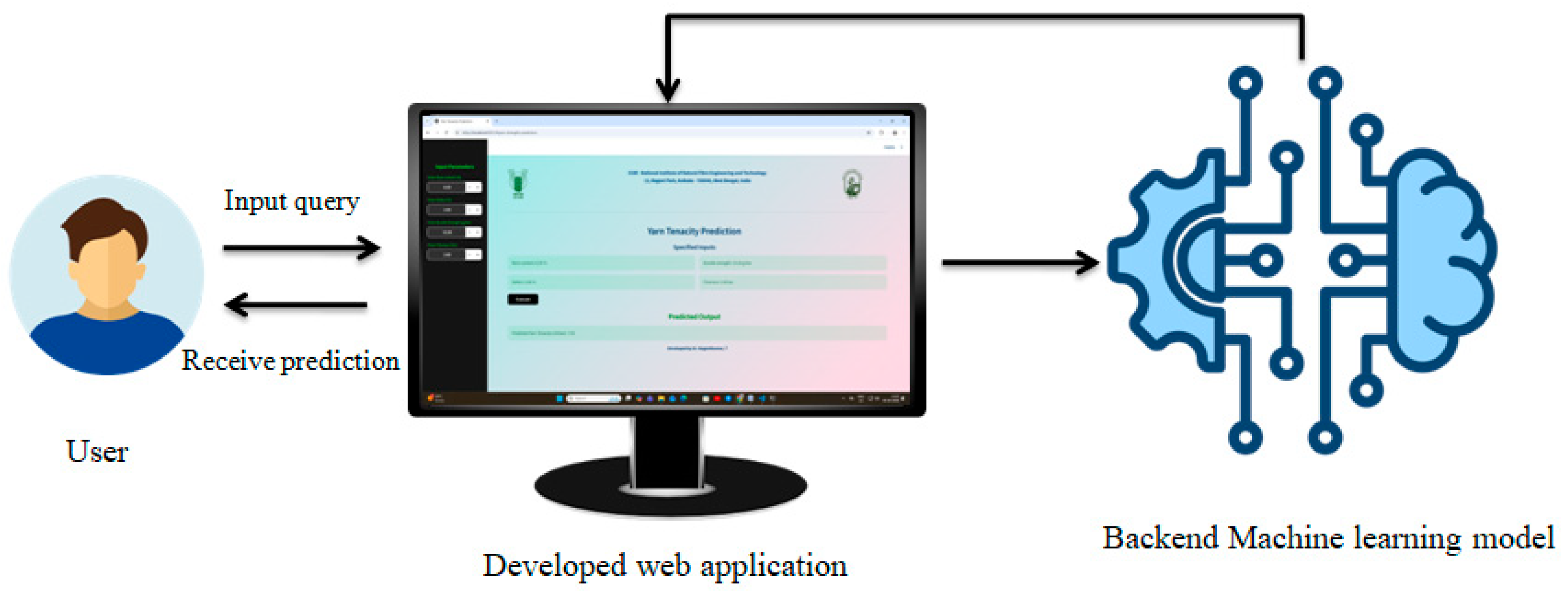
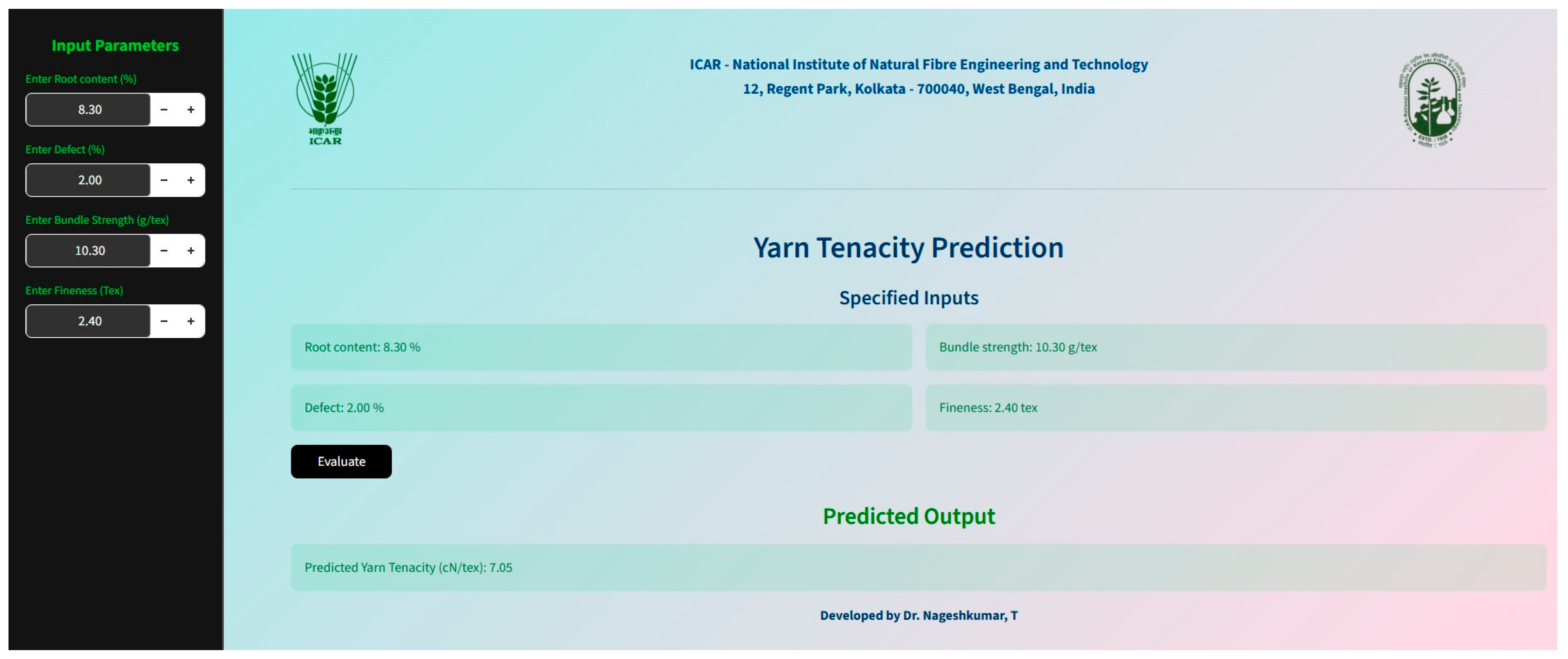
The machine learning models are powerful predictive tools but can often be challenging and difficult to interpret. Deploying these models within a suitable web application significantly improves their accessbility and usability. The best metaheuristic optimzed machine learning model was further integrated into a interactive web application called Streamlit. Streamlit is a Python-based framework that enables rapid build and sharing of interactive web applications. The best RFR, optimized through metaheuristic techniques, was saved using Python’s pickle module to allow efficient loading within the Streamlit app. The flowchart showing the interaction of Streamlit web application with best model is shown in Figure 3. The application provoides a userfriendly interface that allows users to enter input critical parameters like root content, bundle strength, defects, fineness. The resulting tenacity is displayed clearly along with the input values to maintain transparency.

3. Results and Discussion

The description of the dataset used for development of machine learning model is given in

Table 4. Dataset description for development of machine learning model.

Index	Independent Parameters				Dependent Parameter
	Root Content (%)	Defect (%)	Bundle Strength (g/tex)	Fineness (tex)	Tenacity (cN/tex)
Mean	10.05	1.49	19.02	3.18	9.99
SD	3.42	0.51	3.88	0.48	2.12
Maximum	20.5	2.89	28.78	4.6	12.64
Minimum	2.3	0.24	7.09	1.8	6.72
25%	7.6	1.12	16.42	2.9	9.27
50%	9.6	1.46	18.95	3.13	10.14
75%	12.3	1.89	21.85	3.5	10.73

. The feature bundle strength has the highest mean (19.02 g/tex) and a significant range of 7.09 g/tex to 28.78 g/tex. This wide range accompanied by standard deviation of 3.88 g/tex indicates moderate variability. The input attribute root content has ranged from 2.3% to 20.5% with standard deviation of 3.42%, indicating moderate variability. These insights establish a solid basis for conducting more detailed exploratory data analysis.

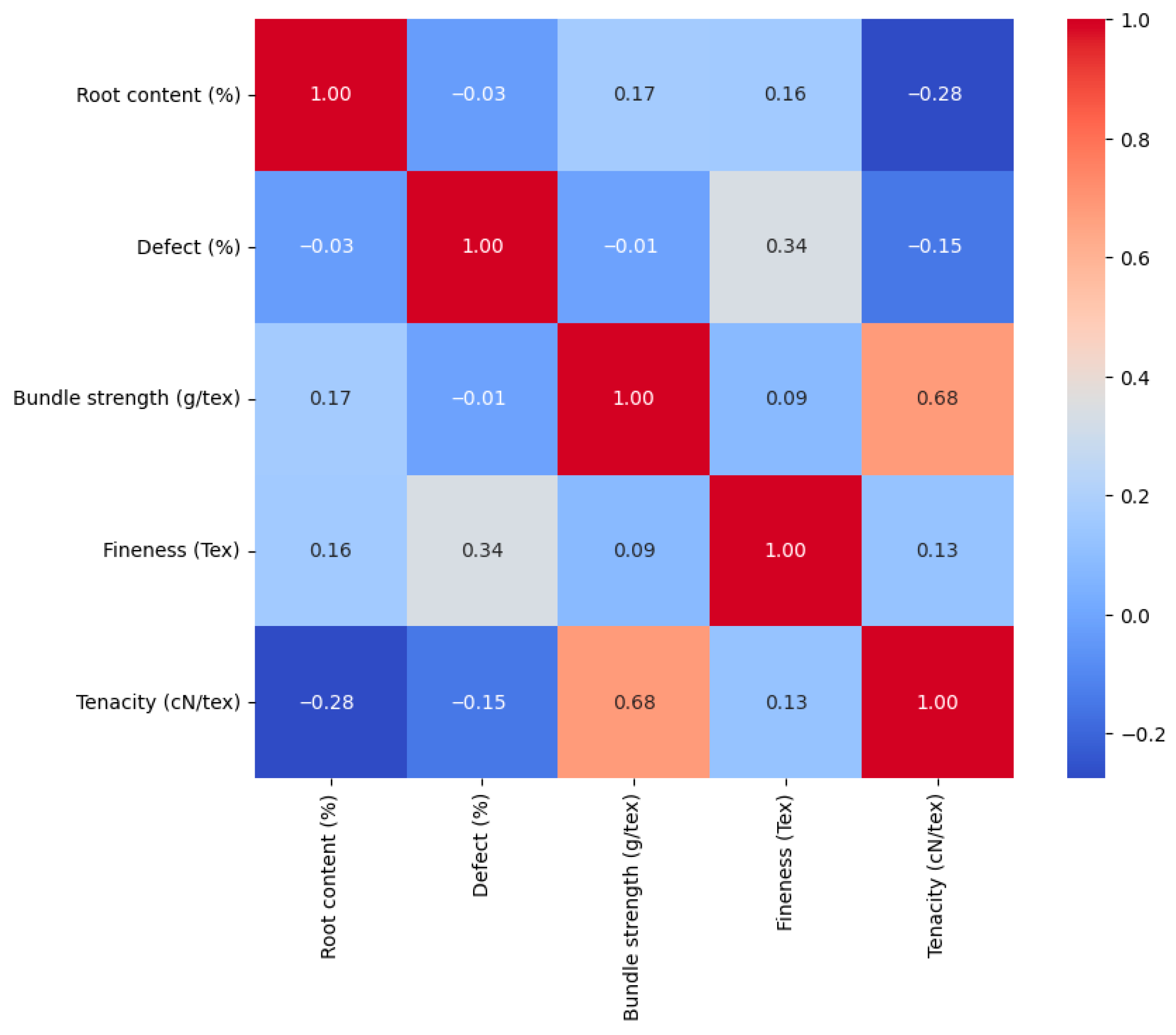
Prior to model training, the Pearson correlation coefficient was employed to assess the interdependence of input and output variables. Figure 4 illustrates the interrelations between input and output variable. The positive correlations are represented by the orange colour, whereas negative correlations are indicated by the blue colour. Notably, the bundle strength of fibre exhibited positive correlation (r= 0.68) with the tenacity of yarn. Conversly, root content and defects showed negative correlation (r = −0.28, r = −0.15), indicating that increased root content and defects resulted in decreases in the tenacity of yarn. The other variable, i.e., fineness showed a weak correlation, with values of correlation coefficient of 0.13.

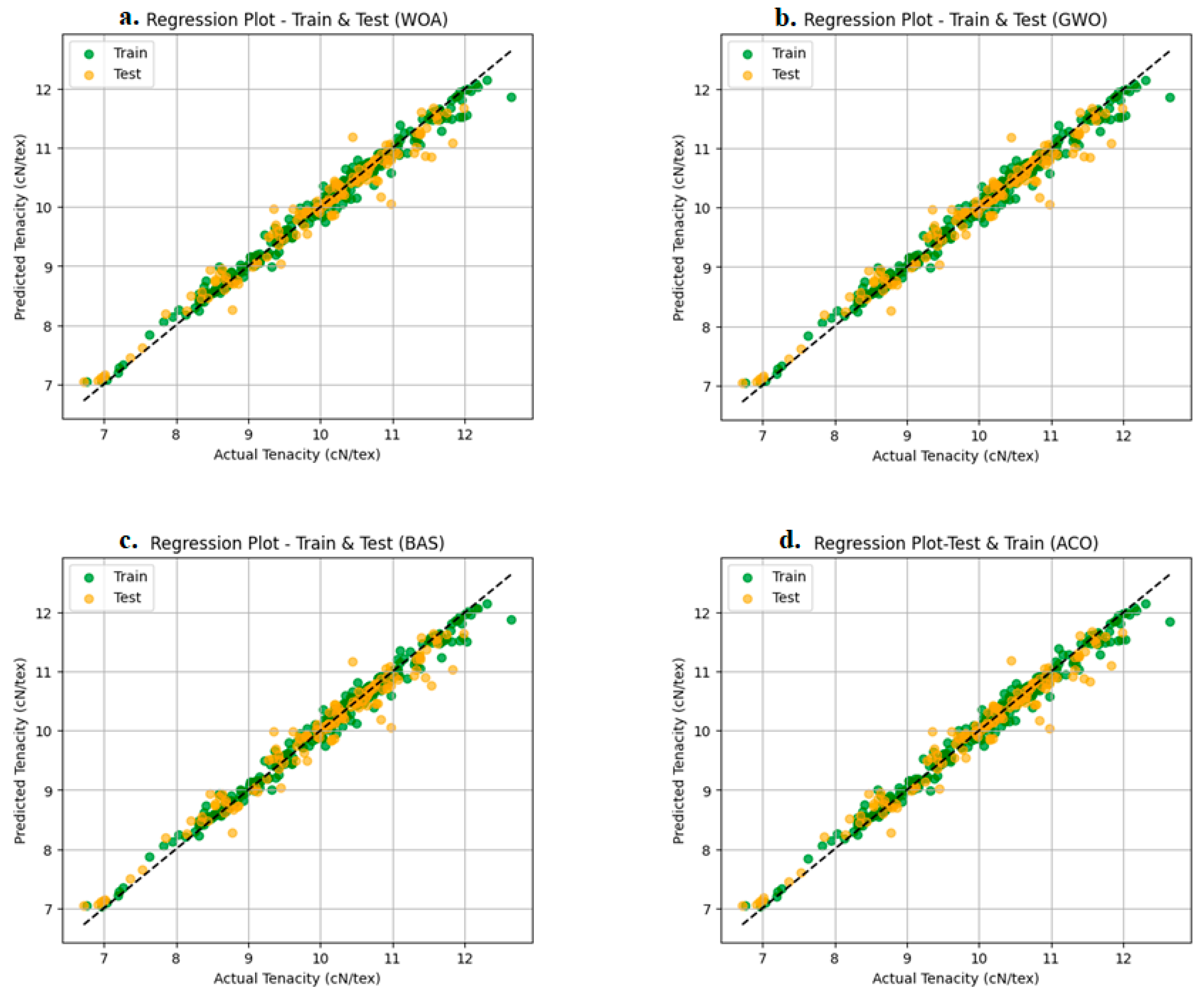
The optimized hyperparameters of the random forest regressor, obtained through tuning with metaheuristic algorithms, are presented in

Table 5. Optimized hyper parameters.

Sl. No.	Model	Optimized Hyperparameters
1	RFR–ACO	n_estimator: 57 max_depth: 12 min_sample_split: 3 min_samples_leaf: 1
2	RFR–WOA	n_estimator: 84 max_depth: 14 min_sample_split: 3 min_samples_leaf: 3
3	RFR–GWO	n_estimator: 58 max_depth: 20 min_sample_split: 3 min_samples_leaf: 2
4	RFR–BAS	n_estimator: 160 max_depth: 11 min_sample_split: 2 min_samples_leaf: 3

. Three statistical indices were employed to assess the prediction performance of each model after obtaining the optimal hyperparameters.

Table 6. Statistical evaluation of developed models.

Sl. No.	Model	Phase	R2	MAE	RMSE
1	RFR–ACO	Training	0.98	0.08	0.11
		Testing	0.95	0.17	0.24
2	RFR–WOA	Training	0.98	0.09	0.14
		Testing	0.95	0.16	0.23
3	RFR–GWO	Training	1.0	0.07	0.10
		Testing	0.96	0.15	0.22
4	RFR–BAS	Training	0.98	0.09	0.13
		Testing	0.95	0.17	0.24

lists the computed values of R², MAE, and RMSE of the developed models. It can be observed from the Table 6 that RFR–ACO, RFR–WOA and RFR–BAS exhibited the same R² value in training and testing phase. The RFR–GWO approach demonstrated R² values of 0.1 and 0.96 for training and testing sets. Likewise, RFR–ACO had 0.082 and 0.17 MAE and 0.11 and 0.24 RMSE for the training and testing phases. The RFR–WOA approach exhibited 0.09 and 0.16 MAE and 0.14 and 0.23 RMSE for the training and testing phases where as RFR–GWO had lower MAE and RMSE values in the training (MAE: 0.77, RMSE: 0.10) and testing phases(MAE: 0.15, RMSE: 0.22). Overall, the developed models showed excellent agreement between the model predicted and actual values of the tenacity of yarn (Figure 5). However, RFR–GWO showed slightly better performance indicators than the other models. The GWO optimizer effectively tuned the hyperparameters of RFR, avoiding local minima and achieving improved generalization [30]. As a results, RFR–GWO yielded higher prediction accuracy.

The developed models were further compared based on their execution time.

Table 7. Execution time of metaheuristic optimized machine learning models.

Sl. No.	Model	Execution Time (s)
1	RFR–ACO	24.60
2	RFR–WOA	19.31
3	RFR–GWO	14.25
4	RFR–BAS	33.40

presents the execution times for all four models, where RFR–ACO, RFR–WOA, RFR–GWO and RFR–BAS required 24.60, 19.31, 14.325 and 33.40 s, respectively. The RFR–GWO model demonstrated the shortest execution time, underscoring its computational efficiency. The shortest execution time of GWO is due to its simple mathematical structures and fewer tuning parameters compared to other metaheuristic algorithms. This structural simplicity minimizes computational overhead, enabling faster convergence while effectively balancing exploration and exploitation during the optimization process [31].

3.1. Shap Interpretability

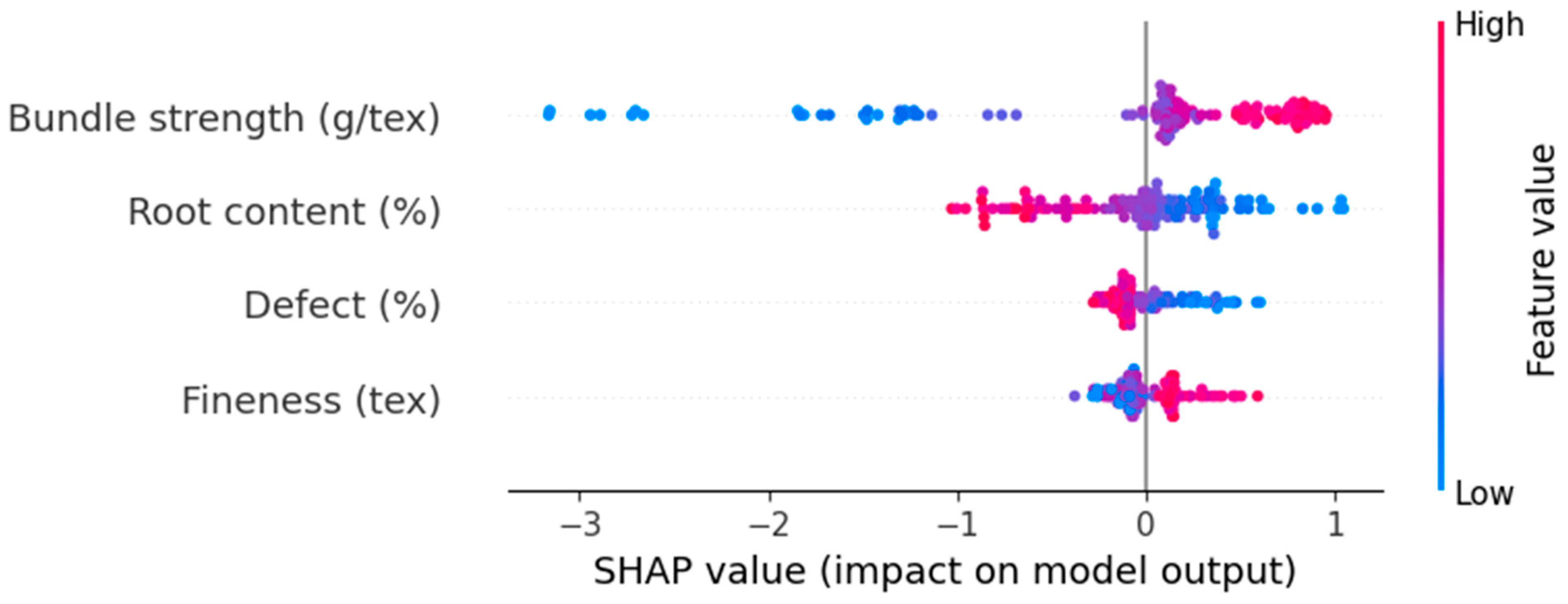
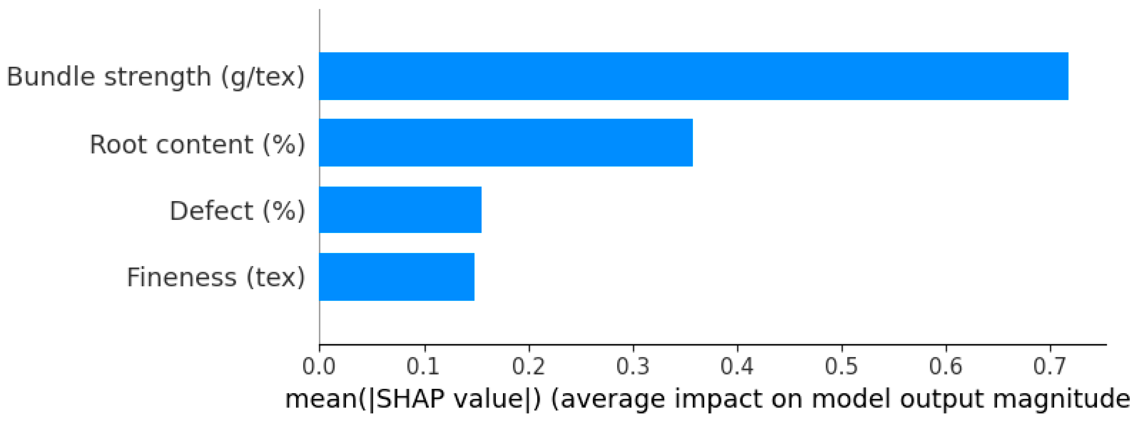
Based on the performance indicators, the RFR–GWO model demonstrated superior prediction accuracy in estimating yarn tenacity, contrary to the other algorithms. Therefore, SHAP analysis was conducted using the results obtained from the RFR–GWO model. Figure 6 shows the SHAP feature importance plot, illustrating how each input feature contributes to the model’s output prediction based on its corresponding SHAP value. It can be observed that bundle strength of jute fibre has the highest SHAP value of +0.71 followed by root content with a SHAP value of +0.35. Similarly, defect and fineness have the lowest SHAP score of +0.15 and +0.14, respectively.

Overall, bundle strength and root content emerged as the most influential parameters in predicting yarn tenacity. The high SHAP value associated with bundle strength indicates a positive relationship—an increase in bundle strength leads to higher yarn tenacity. Similar findings have been reported by Paul [32] and Saha et al. [33]. The root content of the fibre was identified as the second most significant factor. Root content is the hard, barky portion of the fibre; it impedes proper processing and spinning, thereby reducing yarn strength [34]. In contrast, the relatively low SHAP values for defect and fineness suggest that these features have a comparatively smaller influence on the model’s predictions. Nevertheless, both parameters remain crucial. Jute fibre defects are generally classified into two types-minor and major defects. Minor defects are usually removed during softening process, where as major defects remain attached to the fibres. Fibre containing major defects is known to diminish yarn tenacity [35]. Generally, for fibres such as cotton, higher strength and finer fineness enhance yarn tenacity when other fibre parameters are held constant. However, in the case of jute fibre, higher strength combined with coarser fineness leads to an increase in yarn tenacity. This behaviour can be attributed to the mesh-like structure of the jute fibre, which remains partially intact during the yarn formation stage [9,32].

Figure 7 displays the SHAP summary plot, which highlights the relaitonship between various input features and their corresponding SHAP value distrubutions. The vertical axis denotes the input features, while the horizontal axis represents their corresponding SHAP values. Each dot represents a data instance, with colour gradients from blue to red indicating the feature’s intensity. This visualization reveals how changes in feature magnitude affect the predicted output value. It can be observed that bundle strength has a SHAP value ranging from −3 to +1.0. This obsevation indiactes that higher the bundle strength strongly increases the model prediction. In root content, dots spread across both positive and negative SHAP values. High feature values (red) appearing on the left (negative SHAP) and low values (blue) on the right (positive SHAP) indicate that a higher root content significantly reduces the model’s predicted output. The SHAP values for defect ranged from −0.5 to +0.3. A higher defect value tends to lower the model prediction. However, its overall influence is relatively smaller. The SHAP values for fineness ranging from −0.2 to +0.2 shows that it isthe least important feature in this study.

3.2. Sobol Sensitivity Analysis

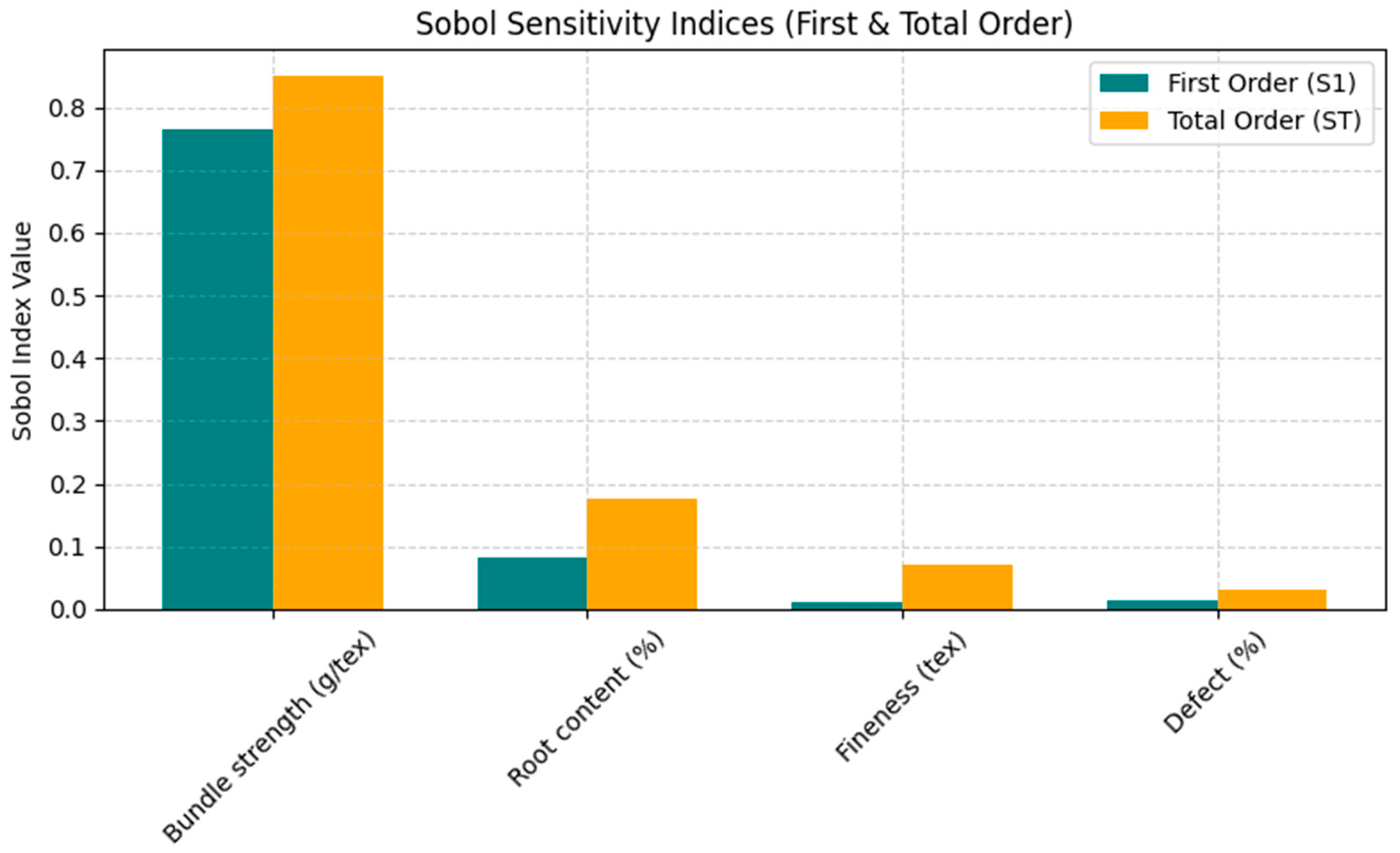
Sobol analysis is a comprehensive, variance-based global sensitivity method that quantifies both the individual influence of each parameter and the extent of their mutual interactions on the model output [36]. The first order (S1) measures the direct contribution of an input variable to the output variance, whereas the total order Sobol index (ST) captures the overall contribution of that variable, including both its individual effect and all interaction effects [37]. Figure 8 depicts the Sobol sensitivity analysis of parameters. Among the variables, bundle strength (g/tex) exhibits the highest influence, with a S1 of approximately 0.77 and ST of about 0.85. This indicates the bundle strength alone explains the majority of the output variance. The second most influential parameter is root content (%) with S1 and ST are 0.08 and 0.17, respectively. The noticeable difference between first order index and total order index values suggests that, although its individual effect is modest, it participates in interaction effects with other variables. In contrast, fineness (tex) and defect (%) show relatively low sensitivity indices (S1 < 0.02 and ST < 0.07), indicating that their individual contributions to output variability are minimal. However, the slight increase in their total-order indices compared to first-order values suggests minor interaction effects

3.3. Streamlit Web App Application

After developing and comparing the metaheuristic optimized RFR, the best performing model RFR–GWO was integrated into a Streamlit web application to provide an intuitive and interactive interface for accessing the predictive capability of the developed model. The development process included designing an interactive interface with dedicated input fields for each variable, enabling users to specify the conditions under which yarn tenacity could be estimated. The developed Streamlit web application is shown in Figure 9. The “Evaluate” button serves as the interactive control of the application, initiating the predictive model to interpret input features and display the calculated yarn tenacity value instantly to the user. This integrated approach enhanced accessibility and user convenience, making the system a practical tool for researchers, manufactures and jute mill operators seeking to predict yarn tenacity with precision.

4. Conclusions

In this study, the hyperparameters of the random forest regression model were optimized using four metaheuristic algorithms: WOA, GWO, BAS and ACO. These hybrid models were designed to forecast jute yarn tenacity from jute fibre properties based on a dataset comprising 414 experimental samples, with 70% data for training and 30% for testing the model. The performance of each model was assessed using four statistical indicators such as R², MAE, RMSE, and computational time. The correlation analysis revealed that the bundle strength of fibre and fineness have a positive correlation, while root content and defects have a negative correlation. Quantitatively, RFR–GWO showed slightly better performance indicators than other models with an R² of 1.0 on training phase and 0.96 on testing phase. Interms of computational time, RFR–GWO completes optimization in 14.25 s. SHAP analysis revealed that the bundle strength and root content of jute fibre are the most influential parameters in predicting yarn tenacity. In contrast, defect and fineness exhibited a smaller influence on yarn tenacity. Sobol sensitivity analysis revealed that bundle strength had astrong direct influence on the model predictions. The RFR–GWO model was integrated into the Streamlit web application, providing an interactive user-friendly interface for real-time prediction of yarn tenacity. It is anticipated that a machine learning-based web application can aid the jute industry and researchers to predict yarn tenacity without actually processing the fibre in the jute mill.

This study demonstrated the effectiveness of a metaheuristic algorithms-optimized RFR model for predicting yarn tenacity from fibre properties. In this study, only yarn tenacity was considered. In the future, parameters such as maximum tensile extension, specific work of rupture and total energy can also be included to provide a more comprehensive analysis of the yarn. Further, the current model is specifically designed for 8-pound yarn (275.6 tex), and future work should focus on developing model suitable for 4 (137.8 tex), 6 (206.7 tex), 10 (344.5 tex), and 16 (551.2 tex) pound jute yarns.

References

Cottrell, J.A.; Ali, M.; Tatari, A.; Martinson, D.B. Effects of fibre moisture content on the mechanical properties of jute reinforced compressed earth composites. Constr. Build. Mater.2023, 373, 130848. [Google Scholar] [CrossRef]
Shambhu, V.B.; Shrivastava, P.; Nageshkumar, T.; Jagadale, M.; Nayak, L.K.; Shakyawar, D.B. Development of gender-friendly power ribboner for extraction of green ribbon/bast from jute plants. J. Nat. Fibers2023, 20, 2250076. [Google Scholar] [CrossRef]
Ullah, A.S.; Shahinur, S.; Haniu, H. Mechanical Properties and Uncertainties of Jute Yarns. Materials2017, 10, 450. [Google Scholar] [CrossRef]
Majumdar, A.; Sarda, S.; Agarwal, T.; Bhattacharyya, R. Decision tree-based machine learning models for yarn quality prediction in the textile industry: A comparative analysis. Soft Comput.2025, 29, 5025–5039. [Google Scholar] [CrossRef]
IS 271: 2020; Textiles—Grading of White, Tossa and Daisee Uncut Indian Jute. Bureau of Indian Standards, Manak Bhavan, 9 Bahadur Shah Zafar Marg: New Delhi, India, 2020.
Mitra, A. Grading of raw jute fibres using criteria importance through inter criteria correlation (critic) and range of value (rov) approach of multi-criteria decision making. J. Nat. Fibers2022, 19, 7517–7533. [Google Scholar] [CrossRef]
Irfan, M.; Khaliq, Z.; Faisal, M.; Qadir, M.B.; Ahmad, F.; Ali, Z.; Alsaiari, M.; Jalalah, M.; Harraz, F.A. Investigating the impact of fiber and yarn structure on yarn tensile properties: A computational approach with artificial neural networks. Mater. Today Commun.2024, 40, 109372. [Google Scholar] [CrossRef]
Bandyopadhyay, S.B. Quality Assessment of jute and mesta yarns from their fiber properties. Text. Res. J.1968, 38, 135–141. [Google Scholar] [CrossRef]
Nageshkumar, T.; Shrivastava, P.; Ammayapan, L.; Jagadale, M.; Nayak, L.K.; Shakyawar, D.B.; Suyambulingam, I.; Senthamaraikannan, P.; Kumar, R. Machine Learning Model Coupled with Graphical User Interface for Predicting Mechanical Properties of Flax Fiber. J. Nat. Fibers2025, 22, 2502662. [Google Scholar] [CrossRef]
Yuan, J.; Li, Y.L.; Chen, S.Y. Prediction of yarn quality based on BP neural network. Adv. Mater. Res.2011, 331, 449–453. [Google Scholar] [CrossRef]
Majumdar, A.; Ghosh, A. Yarn strength modelling using fuzzy expert system. J. Eng. Fiber Fabr.2008, 3, 61–68. [Google Scholar] [CrossRef]
Pattanayak, A.K.; Luximon, A.; Khandual, A. Prediction of drape profile of cotton woven fabrics using artificial neural network and multiple regression method. Text. Res. J.2011, 81, 559–566. [Google Scholar] [CrossRef]
Unal, P.G.; Ureyen, M.E.; Armakan, D.M. Predicting bursting strength of plain knitted fabrics using ANN. In International Conference on Agents and Artificial Intelligence; SciTePress: Setúbal, Portugal, 2010; Volume 2, pp. 615–618. [Google Scholar]
Chattopadhyay, R. Artificial neural networks in yarn property modeling. In Soft Computing in Textile Engineering; Woodhead Publishing: Delhi, India, 2011; pp. 105–125. [Google Scholar]
Lightstone, J.P.; Chen, L.; Kim, C.; Batra, R.; Ramprasad, R. Refractive index prediction models for polymers using machine learning. J. Appl. Phys.2020, 127, 215105. [Google Scholar] [CrossRef]
Malik, S.A.; Farooq, A.; Gereke, T.; Cherif, C. Prediction of blended yarn evenness and tensile properties by using artificial neural network and multiple linear regression. Autex Res. J.2016, 16, 43–50. [Google Scholar] [CrossRef]
García-Nieto, P.; García-Gonzalo, E.; Graciano-Uribe, J.; Arbat, G.; Duran-Ros, M.; Pujol, T.; Puig-Bargués, J. Optimised random forest for predicting bed expansion and pressure drop in media filter backwashing. Biosyst. Eng.2025, 256, 104189. [Google Scholar] [CrossRef]
Ge, P.; Yang, O.; He, J.; Liu, Z.; Chen, H. Metaheuristic algorithms-optimized machine learning models for FRP-concrete interfacial bond strength prediction. Adv. Eng. Softw.2025, 208, 103971. [Google Scholar] [CrossRef]
Hassan, H.M. Metaheuristic-driven optimization of machine learning models for predicting principal dimensions of container ships. J. Ocean Eng. Mar. Energy2025, 12, 459–483. [Google Scholar] [CrossRef]
Zhang, B.; Song, J.; Zhao, S.; Jiang, H.; Wei, J.; Wang, Y. Prediction of yarn strength based on an expert weighted neural network optimized by particle swarm optimization. Text. Res. J.2021, 91, 2911–2924. [Google Scholar] [CrossRef]
Song, J.; Fan, T. Yarn Hairiness Prediction by Generalized Regression Neural Network based on Harris Hawk Optimization. J. Inst. Eng. India Ser. E2022, 103, 347–355. [Google Scholar] [CrossRef]
Hu, S.; Zhang, G.; Zhao, X.; Li, Z.; Li, W. A method for yarn quality fluctuation prediction based on multi-correlation parameter feature subspace mechanism in spinning process. J. Eng. Fiber Fabr.2023, 18, 15589250231208703. [Google Scholar] [CrossRef]
Nageshkumar, T.; Saha, B.; Sardar, G. Digital instruments for precise grading of jute fibre. Indian Farming2024, 74, 32–34. [Google Scholar]
IS 1670: 1991; Textiles—Yarn—Determination of Breaking Load and Elongation at Break of Single Strand. Bureau of Indian Standards, Manak Bhavan, 9 Bahadur Shah Zafar Marg: New Delhi, India, 1991.
Mirjalili, S.; Lewis, A. The whale optimization algorithm. Adv. Eng. Softw.2016, 95, 51–67. [Google Scholar] [CrossRef]
Mirjalili, S.; Mirjalili, S.M.; Lewis, A. Grey wolf optimizer. Adv. Eng. Softw.2014, 69, 46–61. [Google Scholar] [CrossRef]
Jiang, X.; Li, S. Beetle antennae search without parameter tuning (BAS-WPT) for multi-objective optimization. arXiv2017, arXiv:1711.02395. [Google Scholar] [CrossRef]
Lundberg, S.M.; Lee, S.I. A unified approach to interpreting model predictions. In Proceedings of the 31st International Conference on Neural Information Processing Systems, NIPS ’17; Curran Associates Inc.: Red Hook, NY, USA, 2017; pp. 4768–4777. [Google Scholar]
Bardhan, A.; Suman, S.K.; Kumar, S.; Lekhraj; Asteris, P.G. An efficient framework of optimized ensemble paradigm for estimating resilient modulus of subgrades. Transp. Geotech.2024, 48, 101315. [Google Scholar] [CrossRef]
Paul, N.G. Relationship of Some Fiber Properties with Yarn-Strength Parameters of Jute. Text. Res. J.1976, 46, 519–521. [Google Scholar] [CrossRef]
Saha, B.; Nageshkumar, T.; Saha, S.C.; Roy, G.; Sarkar, A.; Sardar, G.; Mondal, J. Development and evaluation of handy jute fibre bundle strength tester. J. Sci. Ind. Res.2022, 81, 113–117. [Google Scholar] [CrossRef]
Singha, A.; Das, A.; Manjunatha, B.S.; Bhowmick, M.; Ray, D.P.; Thakur, A.K.; Biplab, S.; Ruby, D.; Robin, D.; Amit, D. Softening of Barky Root Cuttings of Jute by Pectinolytic Bacterial Strains for Better Spinability and Industrial Uses. Econ. Aff.2022, 67, 439–444. [Google Scholar] [CrossRef]
Nageshkumar, T.; Shrivastava, P.; Saha, B.; Subeesh, A.; Shakyawar, D.B.; Sardar, G.; Mandal, J. Defects identification in raw jute fibre using convolutional neural network models. J. Text. Inst.2024, 115, 835–843. [Google Scholar] [CrossRef]
Saltelli, A.; Ratto, M.; Andres, T.; Campolongo, F.; Cariboni, J.; Gatelli, D.; Saisana, M.; Tarantola, S. Global Sensitivity Analysis: The Primer, 1st ed.; John Wiley & Sons: Chichester, UK, 2008. [Google Scholar]
Wan, H.; Xia, J.; Zhang, L.; She, D.; Xiao, Y.; Zou, L. Sensitivity and Interaction Analysis Based on Sobol’ Method and Its Application in a Distributed Flood Forecasting Model. Water2015, 7, 2924–2951. [Google Scholar] [CrossRef]
Figure 1.
Process of yarn production.
Figure 2.
Flowchart of metaheuristic algorithm optimized machine learning model.
Figure 3.
Flowchart of the developed Streamlit web application.
Figure 4.
Heat map of correlation matrix.
Figure 5.
Actual vs. predicted plot in training and testing phase. ((a) WOA; (b) GWO; (c) BAS; (d) ACO).
Figure 6.
SHAP features importance plot.
Figure 7.
SHAP summary plot.