Loop Order Analysis of Weft-Knitted Textiles

Abstract

In this paper, we describe algorithms that perform loop order analysis of weft-knitted textiles, which build upon the foundational TopoKnit topological data structure and associated query functions. During knitting, loops of yarn may be overlayed on top of each other and then stitched together with another piece of yarn. Loop order analysis aims to determine the front-to-back ordering of these overlapping loops, given a stitch pattern that defines the knitted fabric. Loop order information is crucial for the simulation of electrical current, water, force, and heat flow within functional fabrics. The new algorithms are based on the assumption that stitch instructions are executed row-by-row and for each row the instructions can be executed in any temporal order. To make our algorithms knitting-machine-independent, loop order analysis utilizes precedence rules that capture the order that stitch commands are executed when a row of yarn loops are being knitted by a two-bed flat weft knitting machine. Basing the algorithms on precedence rules allows them to be modified to adapt to the analysis of fabrics manufactured on a variety of knitting machines that may execute stitch commands in different temporal orders. Additionally, we have developed visualization methods for displaying the loop order information within the context of a TopoKnit yarn topology graph.

1. Introduction

Throughout history, knitting as a manufacturing technique has been mostly used for clothing. However, knitted textiles offer great promise in other applications due to their mechanical and physical properties. While knitted textiles have become increasingly important to many industries (e.g., medical, military, etc.) in the last decades, the lack of computer modeling and simulation tools have limited the ability of knitted textiles to be widely deployed. There is a need to robustly design and model knitted textiles in a manner similar to those used for vehicles, buildings, and bridges. The TopoKnit system [1,2] provides significant progress toward this goal by implementing a foundational topological representation of knitted fabrics that supports modeling, simulation, and analysis.

The work presented here builds upon the yarn-based topological structures available in TopoKnit by expanding its query and analysis capabilities, thus capturing additional topological relationships present in knitted fabrics manufactured on a two-bed flat weft knitting machine. Specifically, we present algorithms that implement loop order analysis of weft-knitted textiles. This analysis aims to determine the front-to-back ordering of overlapping yarn loops, given a stitch pattern that defines a knitted fabric.

Expanding our understanding of the topology of weft-knitted textiles, not only advances the correctness and robustness of their associated geometric models, but also contributes to the development and application of knitted structures. Loop order information is crucial for the simulation of electrical current, water, force, and heat flow, as well as for determining fabric properties such as density and porosity [3,4,5,6]. Additionally, a loop order analysis capability contributes to the development of inverse design, the process of determining the stitch instructions that would produce a fabric with desired properties.

Since knitted textiles are composed of consecutive connected rows of intertwined yarn loops, we assume and observe that knitting machines execute stitch instructions row-by-row. However, the order in which these stitch instructions are executed within a row can be arbitrary, i.e., there is no inherent order in which stitch instructions must be carried out. Thus, the algorithms described in this paper are based on the assumption that stitch instructions in each row of a stitch pattern can be executed in any temporal order, depending on the type of the knitting machine performing the instructions. To keep our algorithms machine-independent, the loop order analysis utilizes precedence rules that capture the order that stitch commands are executed when a row of yarn loops are being knitted by a two-bed flat weft knitting machine. The loop order algorithm first determines which loops are brought to a specific location. Then, by analyzing the stitch instructions used to manipulate the loops and by applying the proper precedence rule, the front-to-back ordering is determined. Additionally, we have developed visualization methods for displaying the order information within the context of a TopoKnit yarn topology graph. The precedence rules presented in this paper were derived by analyzing knitting simulations in the Shima Seiki SDS-One APEX3 KnitPaint system (Wakayama, Japan). Since the precedence rules are a variable in the algorithms, they can take different values when modeling/analyzing the fabrics produced by different two-bed flat weft knitting machines. This keeps our approach knitting-machine-independent.

The remainder of the paper is structured as the following. In Section 2, we present related work and its relationship to the presented work. In Section 3, we provide a description of the weft-knitting process and the stitch commands utilized during machine knitting. In Section 4, we give a summary of the TopoKnit system. In Section 5, we detail our algorithms for performing yarn order analysis. In Section 6, we describe the algorithms developed to visualize yarn order information with the context of TopoKnit’s topology graph. In Section 7, we detail the tests that were performed to validate our yarn order analysis and include some of the test results. Finally, in Section 8, we summarize our research and present directions for future work.

2. Related Work

Meissner and Eberhardt developed KnitSim, a pioneering system in modeling and visualizing knitted fabrics [7,8]. This system takes Stoll knitting machine commands as input and outputs an explicit topological representation of the knitted textiles generated from the input commands. A 2D geometric layout of the knitted fabric is generated through a relaxation process making assumptions about the length of yarns between crossings. While this work was promising for its time, it does have some limitations. The approach required a full simulation of the knitting process and imposes constraints that limit the complexity of the modeled knitted structures. The lack of available technical detail hinders the evaluation of the generality and robustness of their approach.

Another similar approach that approximates the 2D layout of knitted textiles is presented by Counts [9]. The developed algorithms employ simulation of the knitting process to generate a graph-based topological representation of the resulting fabric and are able to extract knitting machine instructions from the graph representation. Similar to the Meissner et al. work, Counts’ work requires a full knitting simulation to generate the graph. The choice to use loops as the fundamental primitive, as well as the small set of supported machine instructions, limits the yarn topology that can be represented.

There has been abundant work on the 3D geometric modeling of yarns in knitted textiles. In efforts to create more realistic models, Kyosev et al. [10] propose a model that considers yarn cross section properties by including the compression of the yarns in the loop. Sherburn, Lin, et al. [11,12] developed a multiscale modeling approach aiming to predict the mechanical properties of knitted textiles. To further explore the unique mechanical properties of knitted textiles, Wadekar et al. [13] developed a yarn-level model for weft-knitted fabrics that can be used in finite element analysis simulations. In recent work, Knittel et al. [14] and Wadekar et al. [15,16] explore helicoid scaffolds as a framework for modeling and analyzing the structure and properties of knitted fabrics.

Kaldor et al.’s cutting-edge work [17,18] simulated entire knitted swatches and garments by modeling the geometry and physics of individual yarns in these items. Inspired by this work, Yuksel et al. [19] and Wu et al. [20] introduce a modeling technique that builds yarn-level geometric models of knitted clothing from polygonal models that represent the surface of the knitted cloth. Part of this work was adapted by Leaf et al. [21] to create an interactive design tool for simulating yarn-level patterns for knit and woven textiles.

Cirio et al. [22] define a topological representation of knitted textiles created by a set of limited stitch commands, some of which are not manufacturable on knitting machines. They introduce a compact and simplified representation of yarn geometry and mechanics, capturing essential yarn deformation in their virtual knitted textiles. Their simulation was integrated into a hybrid yarn-triangle model by Casafranca et al. [23]. In related work, Kapllani et al. [1] developed a topological model, TopoKnit, a process-oriented representation that defines a foundational data structure for representing the topology of weft-knitted textiles at the yarn scale. This representation allows for additional topological and manufacturability and stability analysis [2].

McCann et al. [24], Narayanan et al. [25,26] and Lin et al. [27] created algorithms for determining knitting machine commands given polygonal models. These algorithms facilitate interactive design and manufacturing of 3D knitted objects. Popescu et al. [28] described an approach for automatically generating a knitting pattern given a 3D model, without being constrained to developable surfaces. Motivated by Narayanan et al. [25], Kaspar et al. [29] introduced an interactive system which allows users of different skill levels to create and customize machine-knitted textiles. Nader et al. [30] introduced KnitKit, a flexible and customizable system aiming to simplify the knitting of 3D objects by isolating the high-level design from the low-level machine-specific knitting instruction generation.

Our work extends a previously developed topological model (Kapllani et al. [1,2]) to provide additional topological information about a knitted fabric based on the manipulations of its yarn loops. Specifically, in this paper, we present analysis algorithms that define and visualize the order of overlapping loops in a knitted fabric. While Cirio et al. [22], Meissner and Eberhardt [7], and Counts [9] presented work that represents yarn topology in knits, none of them performed any kind of loop ordering determination. Our work produces unique modeling information (loop order) that does not require a full simulation of the knitting process.

3. Fabrication of Weft-Knitted Textiles

A fundamental unit of knitted textiles is the yarn loop. A loop is created when a yarn is drawn through a previously existing loop, as seen in Figure 1. When this process is repeated across a row, and then subsequently again in other rows, the fabric is formed. The actions that create a loop or modify an existing loop are specified by stitch instructions. The two simplest/most common stitch instructions are the Knit and the Purl stitches. As viewed from the front side of the knitting machine, when a yarn is drawn through the loop(s) held on a needle from back to front to form a new loop, a Knit stitch is created, as shown in Figure 2b. When the direction that the yarn is drawn is front to back, a Purl stitch is created, as shown in Figure 3b. A Purl stitch is simply the back side of a Knit stitch. Additionally, a number of other stitch instructions can be executed, which may be combined to produce a vast variety of knitted textiles. These stitches include:

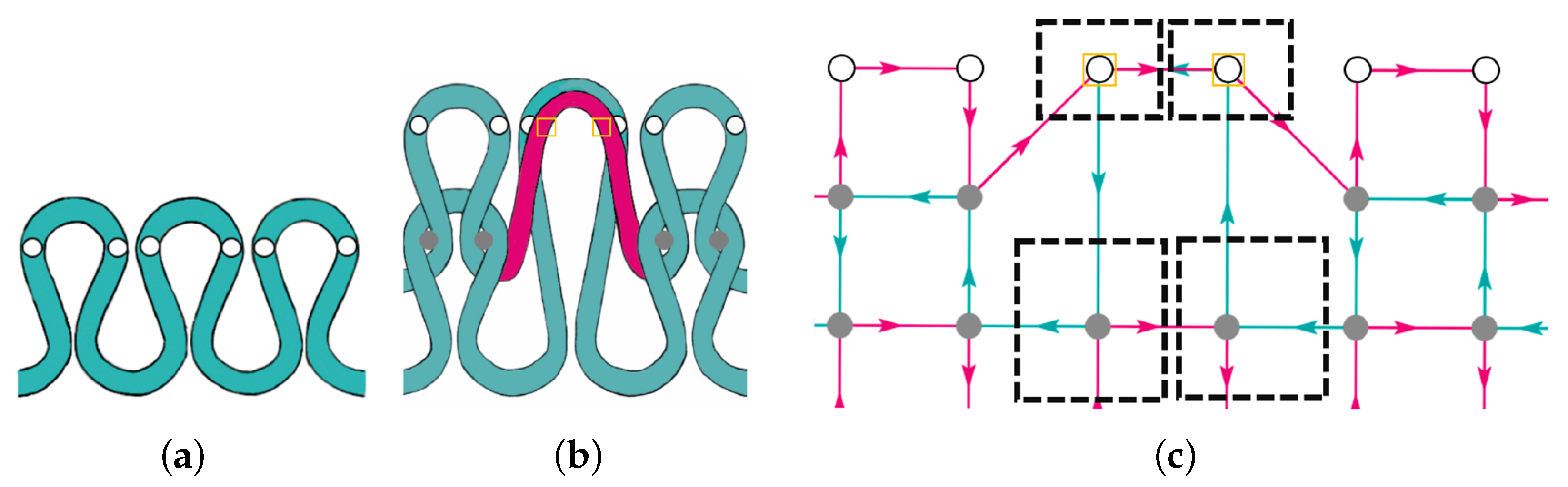
3.1. Front and Back Transfer Stitches

A Transfer stitch is produced when a Knit or Purl stitch is created and then its head loop is transferred, via a sequence of needle bed transfers and rackings, to another needle location. Whether the stitch created is a Knit or Purl determines the type of Transfer stitch. A Front Transfer stitch transfers the head of a Knit stitch and a Back Transfer stitch transfers the head of a Purl stitch (see Figure 4b and Figure 5b respectively).

The Transfer stitches presented in Figure 4b and Figure 5b transfer the loop one needle to the left; however, depending on the type of Transfer stitch, there can be up to three loop movements to the left or right. When a new yarn comes to the needle holding the transferred loop, both overlapping loops will be knit together. The transferred loops are highlighted in magenta in Figure 4b and Figure 5b.

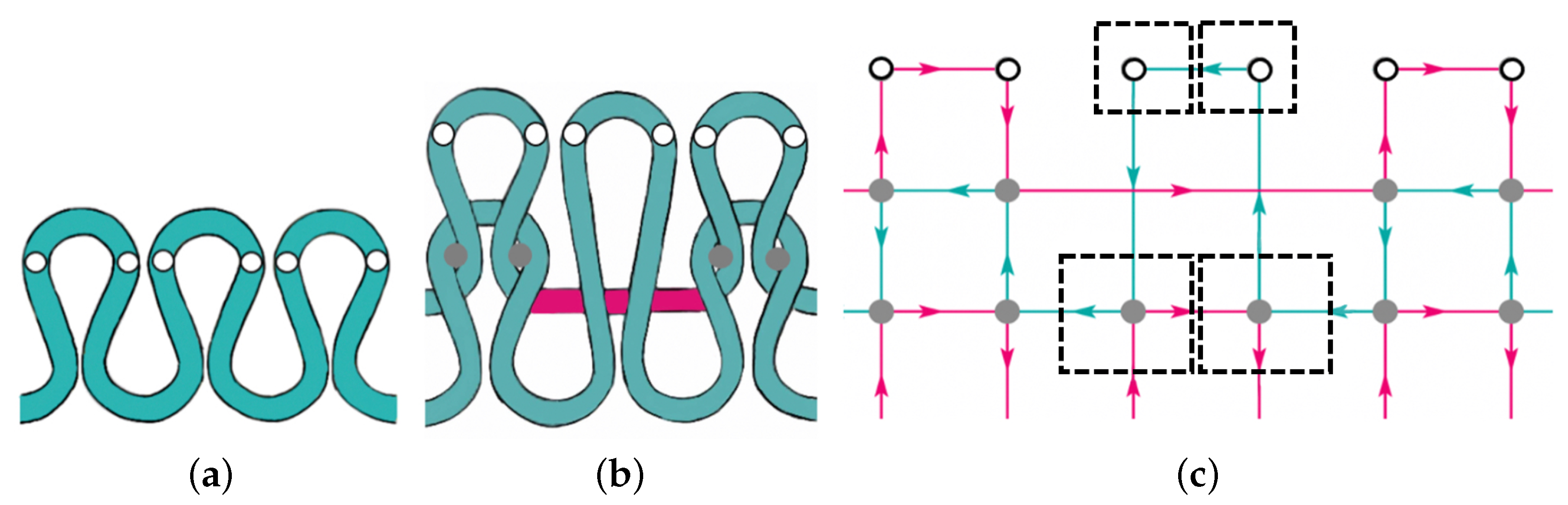
3.2. Front and Back Tuck Stitches

A Tuck stitch is created when a yarn is tucked onto the needle and pulled up, instead of being pulled through the held loop. The tucked loop is held on the needle together with the loop from the previous row, as shown in Figure 6b and Figure 7b. Executing a Back or Front Tuck stitch will determine if the tucked loop is positioned in front of or in back of the held loop, respectively. The needle holds both loops, which will be knitted together when a stitch instruction is executed above it on the next row. The tucked loops are highlighted in magenta in Figure 6b and Figure 7b.

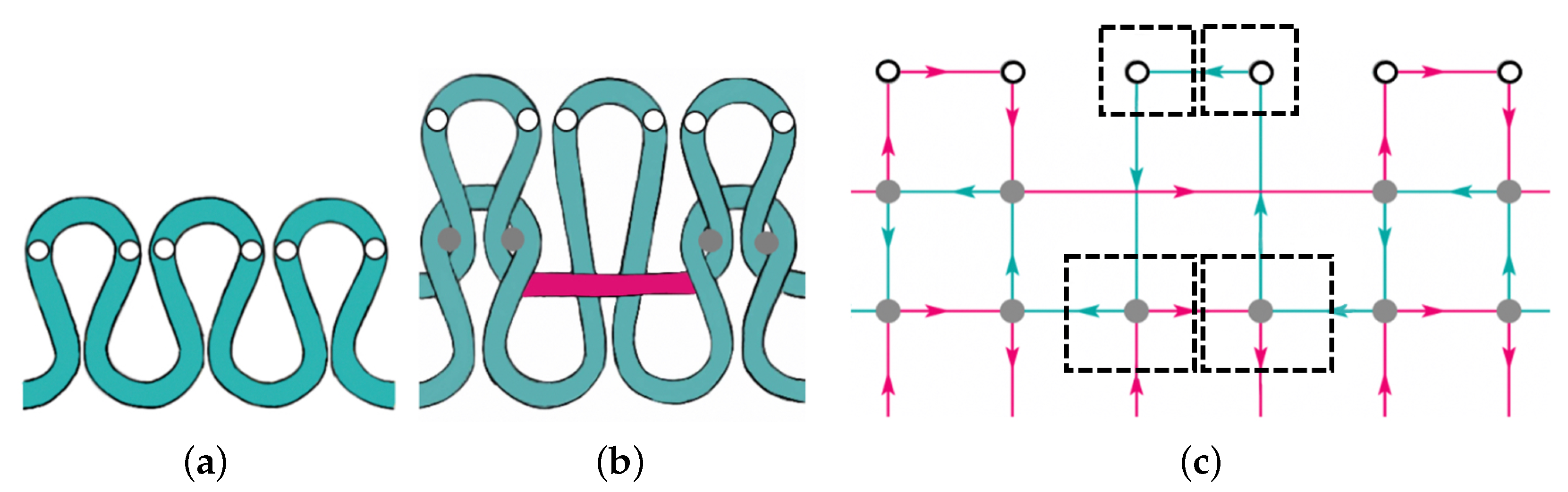
3.3. Front and Back Miss Stitches

Similarly to the Tuck stitch, during the execution of a Miss stitch, the needle holds the loop from the previous row, but the new yarn is not hooked by the needle. Instead, the yarn passes by, creating a horizontal segment of yarn across the front or the back of the held loop. Executing a Back or Front Miss stitch will determine whether the yarn passes in front of or in back of the held loop, respectively. The resulting horizontal yarns are highlighted in magenta in Figure 8b and Figure 9b.

3.4. Empty Stitch

An Empty stitch specifies that no machine operation will be executed for a specific needle. In our work, we assume that Empty stitches cannot be completely surrounded by non-Empty stitches, i.e., Empty stitches only occur outside the borders of the fabric. Therefore, no yarn passes by nor is looped on the needle at that stitch location.

These nine stitches (Knit, Purl, Front and Back Transfer, Front and Back Tuck, Front and Back Miss, and Empty) are the fundamental stitches needed to create most knitted textiles and can be combined to generate complicated knitted patterns. TopoKnit supports all of these stitches, thus allowing for a broad representation of intricate knitted fabrics.

4. TopoKnit

TopoKnit is a topological model of knitted textiles defined within a process-oriented space that represents aspects of the fabric itself, as well as the processes that manipulate the fabric during knitting (Kapllani et al. [1]). The primary primitives of this modeling space are yarn intertwinings and the yarns that connect them. The complexity of a yarn intertwining is encapsulated in a primitive called the Contact Neighborhood (CN). There are three types of CNs: the potential CN (PCN), the actualized CN (ACN), and the unanchored CN (UACN). When a loop is formed, two PCNs are created. When the yarn comes back to the location of these PCNs and is pulled through the existing loop to form a new loop (creating two intertwinings), the PCNs are actualized to ACNs. An ACN is defined by a contact point and four directed incident edges. See the gray (ACNs) and white (PCNs) disks in Figure 2c, which are defined by a Knit stitch. Depending on the loop manipulations during the knitting process, PCNs can be actualized at their creation location or at another location in the fabric grid. An example of the latter would be the PCNs created by Transfer stitches, as seen in Figure 4 and Figure 5. The third CN type, a UACN, is created when the yarn is grabbed by the needle, but the loop’s legs are not intertwined with (i.e., anchored by) another loop from directly below. The squares in Figure 10c represent UACNs. These CNs are connected horizontally with their neighbors along the magenta edge flowing from left to right and therefore are unanchored.

TopoKnit defines a data structure which stores information about these CNs, as well as their mappings, i.e., movements within the fabric grid. For each CN $(i,j)$, four parameters are stored in the data structure. They are: stitch type (ST), actualization value (AV), movement vector (MV), and yarn path index (YPI). The first parameter is the only location-based parameter and it specifies the type of stitch executed at location $(i,j)$ when a CN (created at or transferred to $(i,j)$) is actualized at the location. The actualization value and movement vector make up the mapping information for each CN. The actualization value shows if a CN has been created at a location $(i,j)$ and if so defines its state. The four actualization parameter values are: PCN, ACN, UACN and E. ’E’ implies that no CN was instantiated at the associated location, i.e., the CN is Empty. The movement vector [$\Delta i$,$\Delta j$] specifies if the CN is being moved vertically or horizontally and by how many units. The YPI parameter stores information about the CN’s location in the yarn path list as a set of indices into the list. The yarn path list consists of a set of locations the yarn passes through in the fabric grid. Having this information stored in the data structure allows for constant-time information access during the analysis stage.

Given a stitch pattern composed of the stitch instructions supported by TopoKnit, populating the data structure is the first step toward the analysis stage. See Figure 10d. The analysis stage consists of algorithms developed to evaluate the data structure and support topological query functions. TopoKnit’s main evaluation routine produces the path of the yarn through the fabric and stores it as a sequential list of grid locations in the fabric. The yarn path may be used to visualize the topology graph of the resulting knitted fabric, as seen in Figure 10c, which is produced from the stitch pattern in (a). Examples of supported topological queries include determining the final location of a CN in the fabric grid, identifying which CNs will ultimately be situated at a particular fabric grid location, returning a list of neighboring CNs, as well as providing a list of topological structures we call open loops. Our current work adds loop order determination to this list. In addition to yarn-level topological analysis, TopoKnit supports manufacturability and structural stability analysis (Kapllani et al. [2]).

5. Loop Order Analysis

A new topological query has been added to the TopoKnit system, specifically the front-to-back order of yarn loops. Due to the manipulations of the yarn during the knitting process, multiple overlapping loops may end up at the same location in the fabric. The final spatial order of these loops (front-to-back) is determined by the temporal order that the loops were manipulated and placed during knitting. The loop order query makes use of this fact, along with the information stored in the TopoKnit data structure to define the spatial order of loops at a location $(i,j)$ in the fabric grid. It is important to note that since we are trying to define the order of loops, our analysis only involves stitch instructions that create new loops, such as Knit (K), Purl (P), Front (FX) and Back (BX) Transfer, and Front (FT) and Back (BT) Tuck Stitch and excludes the Miss (M) stitch.

Both hand and machine knitting are row-by-row processes. Therefore, the loop order analysis algorithms assume that the stitch commands are processed row-by-row. The execution order for stitches within a row depends on the type of knitting machine performing them. To represent and isolate this machine dependency in our algorithms, precedence rules are introduced as input to the loop order algorithm. The precedence rules consist of a sequence of stitch instructions starting with the stitch instruction that is executed first in a row of instructions and ends with the stitch instruction that is executed last. The precedence rules can be easily changed when analyzing the fabric manufactured by a specific knitting machine.

The first step of the loop order query determines which loops are brought to the queried location in the fabric grid. The loops that end up at the location in the fabric may have originated from multiple lower rows in the fabric. When analyzing these loops, they are processed row-by-row, with lowest originating row being processed first. A precedence rule is then applied to determine the order of stitch command execution, and therefore the ordering of the associated yarn loops, for that row. The stacked loops from one row are then recursively concatenated with loops that are ordered from successive rows.

5.1. Precedence Rules

For each type of knitting machine, precedence rules specify the temporal order that stitch instructions in a single row of a stitch pattern are executed by the machine. The examples presented in this paper use precedence rules that were inferred by analyzing simulations of different stitch patterns in the Shima Seiki SDS-One APEX3 KnitPaint system. Over one hundred patterns were simulated and examined to determine the order that Shima Seiki knitting machines execute Knit, Purl, Front and Back Transfer, and Front and Back Tuck stitches in a row of stitches. The order that these stitches are executed depend on what types of stitches exist in a row. Knit, Purl, and Transfer (K-P-X) stitches are executed as a block. If the row contains a Back Tuck (BT), the K-P-X block is executed first, then followed by the execution of the BT stitch. This is seen at location (4,3) and (5,3) in Figure 11 and Figure 12. If the row contains a Front Tuck (FT), the FT stitch is executed first and the K-P-X block of stitches is then executed.

Therefore, there are two precedence rules for the K-P-X block of stitches, depending if the block contains Front Transfer (FX*) or Back Transfer (BX*) stitches. Knit stitches are always executed first and Purl stitches are executed last in the block. What determines the precedence of the block is the presence of Front Transfer stitches, with or without the inclusion of Back Transfer stitches. The first rule accounts for the existence of Front Transfer stitches in the row being processed, whereas the second accounts for all Transfer stitches in the row being Back Transfer stitches. Within these rules, the direction of the transfer, the number of needle positions shifted (shift units) and the stitch type (FX or BX) determine the execution order of the stitches. In the first rule, the smaller the shift unit, the higher the precedence of the Transfer stitch instruction, i.e., the sooner the stitch is executed (See locations $(4,2)$ and $(5,2)$ in Figure 13 and Figure 14). For stitches with equal shift units, the left movement direction precedes the right one (See locations $(6,5)$ and $(7,5)$ in Figure 11 and Figure 15), and for stitches with equal shift units and direction, Front Transfer stitches precede Back Transfer stitches. Given this information, the first precedence rule, from highest to lowest precedence, for K-P-X blocks is

$$(K,FXL,BXL,FXR,BXR,FXL2,BXL2,FXR2,BXR2,FXL3,BXL3,FXR3,BXR3,P).$$

Similar to the first rule, the second precedence rule uses shift units and movement direction to define the execution order of blocks containing only Knit, Purl, and Back Transfer stitches. However, contrary to the first rule, the higher the shift unit is, the higher the execution precedence of the stitch instruction is in the second rule. For stitches with equal shift units, the left movement direction precedes the right one. Given this information, the second rule for K-P-X blocks with only Back Transfers is

$$(K,BXL3,BXR3,BXL2,BXR2,BXL,BXR,P).$$

These precedence rules are codified in Algorithm 1.

Algorithm 1$DETERMINE\_RULE(rowj,pattern)$ Returns the precedence rule for row j in pattern

1:  rule = {}   2:  currentRow = pattern[*,rowj]   3:  if FX* in currentRow then   4:        rule = (K,FXL1,BXL1,FXR1,BXR1,FXL2,BXL2,FXR2,BXR2,FXL3,BXL3,FXR3,BXR3,P)   5:  else if BX* in currentRow then   6:        rule = (K,BXL3,BXR3,BXL2,BXR2,BXL1,BXR1,P)   7:  else   8:        rule = (K,P)   9:  if FT in currentRow then 10:        rule = FT + rule                            ▹ Front Tuck has highest precedence 11:  else if BT in currentRow then 12:        rule = rule + BT                          ▹ Back Tuck has the lowest precedence        return rule

5.2. Contact Neighborhood Order

As noted in Section 3, a loop in TopoKnit is defined by a list of edges that adhere to certain constraints. An edge defines a yarn connection between two CNs. Thus, the order of loops at a location $(i,j)$ mirrors the order of head CNs of the loops present at that location. Therefore, our algorithm (Algorithm 2) for determining loop order finds the order of CNs at a given location in the fabric grid. The algorithm begins by finding all of the CNs that end up at the location (if any) (Line 2, Algorithm 2). This is accomplished with the CNS_AT algorithm, which is a slight modification of the ACNS_AT algorithm (Algorithm 5 in [1]). Specifically, the CNS_AT algorithm returns all CNs at a location by omitting the condition that the CN’s actualization value be “ACN”.

Algorithm 2$YARN\_ORDER(i,j,pattern,DS)$ Return the list of CNs at location $(i,j)$ ordered by their spacial position (front-to-back).

1:  orderedCNs = []   2:  CNList = CNS_AT(i, j, DS)                              ▹ CNs at location $(i,j)$   3:  if CNList == [] then                                ▹ No CNs at this location   4:        PRINT(“There are no CNs at this location")   5:        return orderedCNs   6:  CNStitchPairs = CN_STITCH_PAIRS(CNList, pattern)    ▹ Define the stitches that create each CN at location (i,j)   7:  sortedCNStitchPairs = SORT_BY_J(CNStitchPairs)         ▹ Sort pairs by the row the CNs were defined at   8:  return YARN_ORDER_RECURSIVE(sortedCNStitchPairs, pattern, orderedCNs)

Each CN is created when a loop is formed by the execution of a stitch instruction. Since the order of CNs depends on the stitches that create them, each CN is paired with the corresponding stitch that formed it. For instance, CNs $(4,3)$ and $(5,3)$ in Figure 11c were formed by the Back Tuck (BT) stitch in the pattern shown in Figure 11a. The pairings between the CNs and the stitch are specified with the helper function CN_STITCH_PAIRS (See Algorithm 3). When a stitch instruction at coordinate m, n) in the stitch pattern is executed, four CN cells are populated in the TopoKnit data structure. Two correspond to two leg CNs ((2m, n), (2m + 1, n)) and two correspond to two head CNs ((2m, n + 1), (2m + 1, n + 1)). See Figure 16. Since only head CNs can be moved in the fabric grid by a stitch, they are considered when determining corresponding stitch instructions. Therefore a head CN located at $(i,j)$ in the CN grid can be associated with a stitch command located at $(i/2,j-1)$, if i is even, and at $\left(\right(i-1)/2,j-1)$, if i is odd. Note that $CNStitchPairs$ is a dictionary where the CN (i,j) IDs are the keys and the corresponding stitch codes are the values.

Algorithm 3$CN\_STITCH\_PAIRS(CNList,pattern)$ Return a dictionary of CN-Stitch pairs given a list of CNs

1:  CNStitchPairs = {}   2:  for (CNi,CNj) in CNList do   3:        n = CNj - 1              ▹ Determine n coordinate of the corresponding stitch in the pattern matrix   4:        if CNi % 2 == 0 then         ▹ Determine m coordinate of the corresponding stitch in the pattern matrix   5:             m = CNi / 2   6:        else   7:             m = (CNi - 1) / 2   8:        correspondingStitch = pattern[m][n]         ▹ Access corresponding stitch at (m,n) in pattern matrix   9:        CNStitchPairs[(CNi,CNj)] = correspondingStitch          ▹ Assign CN-stitch pair for the current CN        return CNStitchPairs

CNs whose final location is $(i,j)$ may be created by stitch instructions within a small neighborhood of the location, possibly from a different row. Since knitting is a sequential process, stitch instructions in lower rows are processed before the ones in higher rows. Therefore, the entries in $CNStitchPairs$ are sorted by their row number, with the algorithm SORT_BY_J (not included here). Stitch pairs from lower rows come before stitches from higher rows and are stored in $sortedCNStitchPairs$.

Once the CN-Stitch pairs have been created and sorted by their row j (Lines 6 and 7), Algorithm 2 determines the CN order at location $(i,j)$ by calling the function YARN_ORDER_RECURSIVE (Algorithm 4), which recursively processes CN-Stitch pairs at location $(i,j)$ row-by-row, starting with the lowest row. For each row of stitch instructions, which is stored in $currentRow$, $DETERMINE\_RULE$ returns the appropriate precedence rule for the current row (Line 4, Algorithm 4), as described in Section 5.1. The function ORDER_ROW_CNS (Algorithm 5) is called to order the CNs in $currentRow$ using the precedence rule in $rule$ (Line 13 and 15, Algorithm 4). ORDER_ROW_CNS sorts the CNs based on the index of its corresponding stitch in the precedence rule.

Algorithm 4$YARN\_ORDER\_RECURSIVE(sortedCNStitchPairs,pattern,orderedCNs)$ Recursive function used to define the order of CNs at location $(i,j)$

1:  if len(sortedCNStitchPairs) != 0 then                          ▹ Process until no CNs are left   2:        currentRow = {}                           ▹ Stores the CN-Stitch pairs for the current row   3:        smallestJ = sortedCNStitchPairs[0].CNj                             ▹ Row being processed   4:        rule = DETERMINE_RULE(smallestJ)                  ▹ Precedence rule for the row being processed   5:         for CN(i,j),stitch in sortedCNStitchPairs do   6:             if j == smallestJ then                         ▹ CN defined in the row being processed   7:                  currentRow[CN(i,j)] = stitch   8:             else   9:                  break 10:        for CN(i,j) in currentRow.keys() do                  ▹ Delete CN-Stitch pairs about to be processed 11:             delete sortedCNStitchPairs[CN(i,j)] 12:        if rule[-1] == BT then                                    ▹ Row contains a BT 13:             orderedCNs = ORDER_ROW_CNS(currentRow, rule) + orderedCNs 14:        else                                        ▹ Row does not contain a BT 15:             orderedCNs = orderedCNs + ORDER_ROW_CNS (currentRow, rule) 16:        return YARN_ORDER_RECURSIVE(sortedCNStitchPairs,pattern, orderedCNs)       ▹ Process the CNs in next row 17:  return orderedCNs

Algorithm 5$ORDER\_ROW\_CNS(currentRow,rule)$ Return ordered CNs in currentRow given a precedence rule

1: stitchIndexCNPairs = []   2: orderedCNs = []   3: for CN(i,j),stitch in currentRow.items() do                ▹ Create pairs of stitch index and CNs for current row   4:       stitchIndexCNPairs.append((rule.index(stitch),CN(i,j)))   5: sortedStitchIndexCNPairs = sorted(stitchIndexCNPairs)]     ▹ Order by the index of stitches in the precedence rule   6: for index, CN(i,j) in sortedStitchIndexCNPairs do                       ▹ Extract ordered CNs   7:       orderedCNs.append(CN(i,j))   8: return orderedCNs

Tuck stitches (Front (FT) and Back (BT)) not only have a precedence relative to the other stitches in their row, but they also affect the precedence of the stitch block that has been ordered in the previous row. As seen in Lines 9 and 10 in Algorithm 1, Front Tuck (FT) has the highest precedence of all the supported stitches, while Back Tuck (BT) has the lowest, seen in Lines 11 and 12. Conversely, when concatenating a new line of stitches (those returned by ORDER_ROW_CNS) containing a Back Tuck (BT) with a previous line ($orderedCNs$), as seen in Lines 12 and 13 of Algorithm 4, the block containing the BT has higher precedence than the stitch block from a lower row. The ordered $currentRow$ is placed before the stitch block from the previous row ($orderedCNs$). If no BT is present in the current row, the previous stitch block ($orderedCNs$) is placed in front of the current row (Line 15, Algorithm 4).

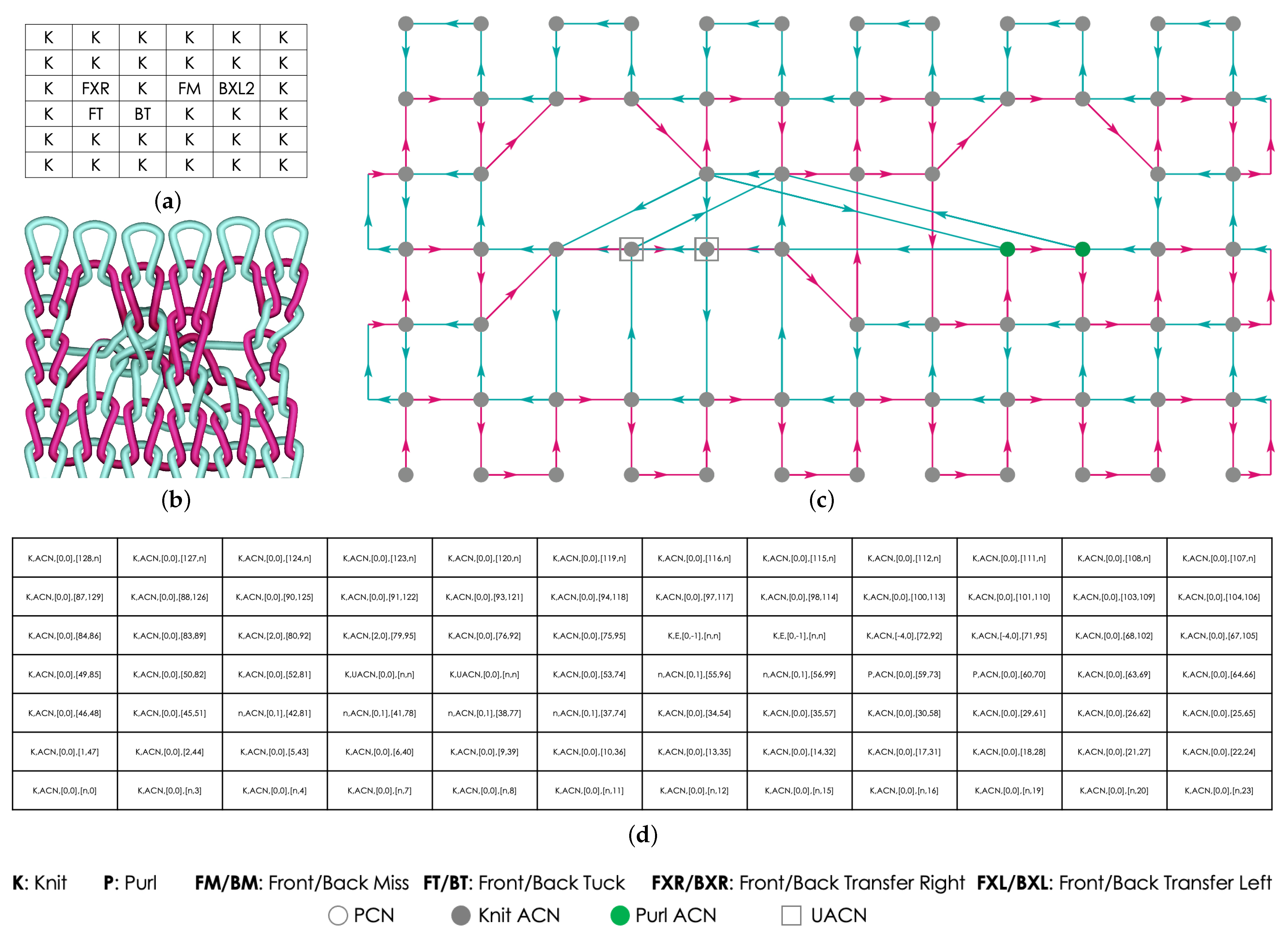
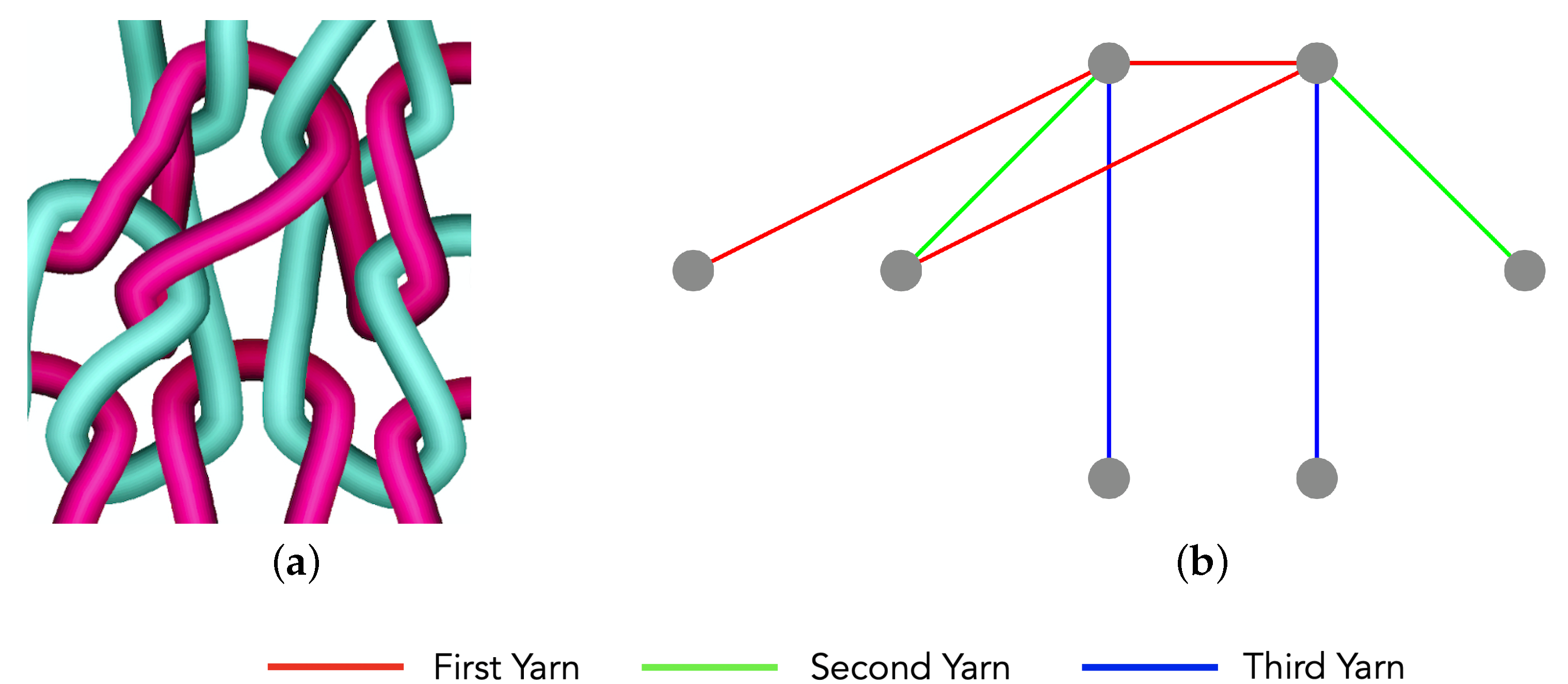
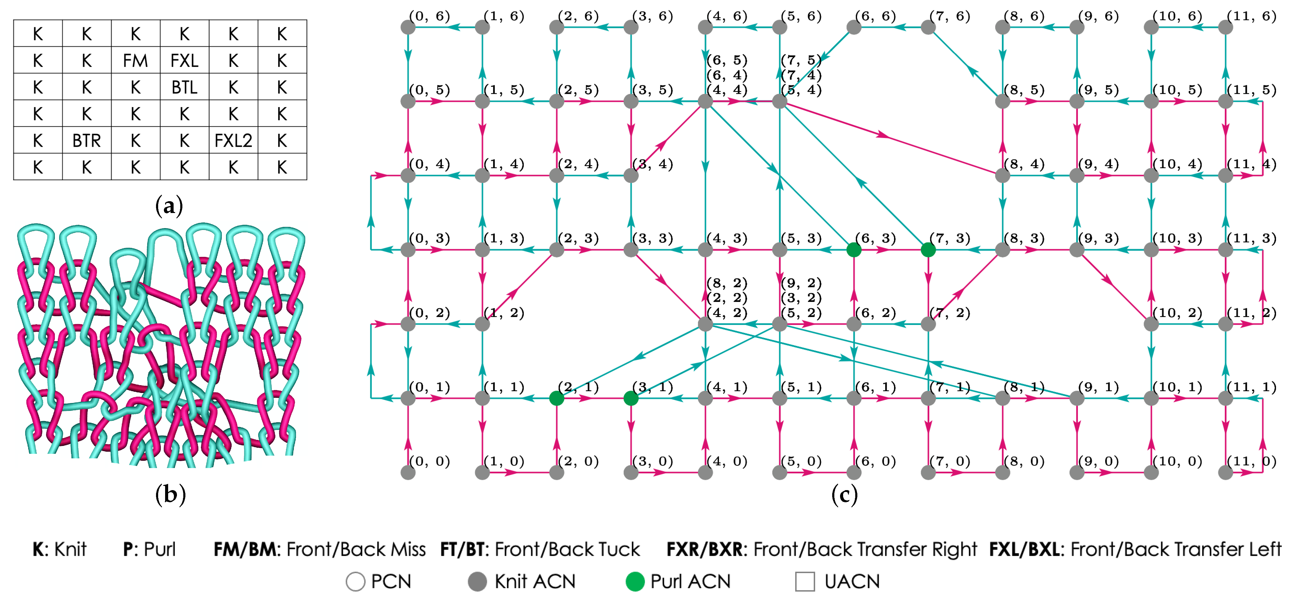
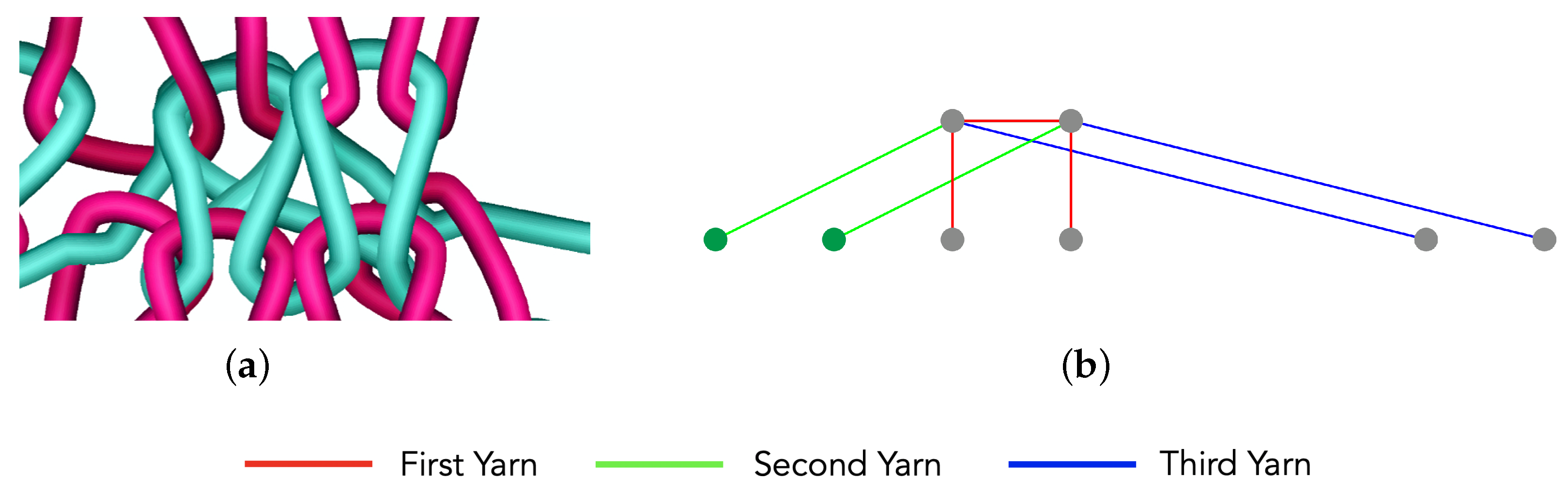
6. Yarn Order Visualization

The algorithms presented in Section 5 describe how the ordering of stacked CNs, and, therefore, yarn loops, is determined for a knitted fabric. This ordering information, provided by the execution of the YARN_ORDER function, has been incorporated into TopoKnit’s yarn topology graph visualization algorithm (Algorithm 7 (DRAW_TOPOLOGY_GRAPH) in Kapllani et al. [1]) in the form of textual data. Examples of these visualizations are provided in the yarn topology graphs in Figure 11c, Figure 13c and Figure 17c. In each $(i,j)$ location in the graphs where at least one CN is present, labels corresponding to the CN order are added. In locations where there are more than one CN, the displayed bottom-to-top order of the CNs corresponds to the order of yarns from front to back.

Zoom-in Visualizations

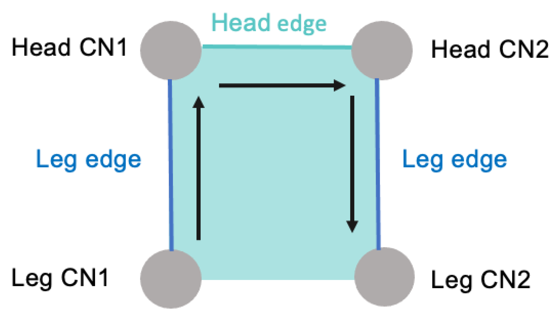
Using textual data to convey loop ordering may not be ideal for all scenarios or users. Therefore, Algorithm 6 was developed to display a zoom-in view of the stacked loops that go through location $(i,j)$, using color instead of textual data to present ordering information. The zoom-in graphs presented in this paper use three colors, where the red loop represents the front loop, the green loop represents the middle loop, and the blue loop represents the back loop. We chose three colors based on the assumption that three is the maximum number of loops a needle can hold without breaking, as described in [2]. Algorithm 6 can be easily modified for a different assumption, i.e., the needle can hold more than three loops, by adding colors to the $yarnColors$ variable accordingly. An example of a zoom-in graph is given in Figure 15b. This figure displays loop ordering at locations $(6,5)$ and $(7,5)$ for the yarn topology graph presented in Figure 11c.

To create a zoom-in graph, the list of ordered CNs at location $(i,j)$ is generated and a yarn color is assigned to each depending on its order position. The zoom-in graph draws the corresponding loop for each CN in their specified order. To ensure that intersections between pairs of yarns are correctly ordered visually, the list of CNs is reversed. Thus, the loops are drawn in a back-to-front order. See Lines 1–7 in Algorithm 6.

Algorithm 6$YARN\_ORDER\_ZOOM\_IN(i,j,pattern,DS)$ Generate a zoom-in topology graph showing the order of loops at location $(i,j)$.

1: yarnColors = [red, green, blue]                          ▹ Front-to-back yarn colors   2: orderedCNs = YARN_ORDER(i, j, pattern, DS)   3: if len(orderedCNs) == 0 then return   4: colorOrderedCNs = []   5: for index, CN in enumerate(orderedCNs) do         ▹ Assign a color to each CN depending on its order   6:      colorOrderedCNs.append([CN, yarnColors[index]])   7: colorOrderedCNs.reverse()                       ▹ Reverse to draw loops from back to front   8: yarnPathList = FOLLOW_THE_YARN(DS)   9: loops, edgeLoopPair, indexLoopPair = DEFINE_OPEN_LOOPS(yarnPathList) 10: while There are CNs in colorOrderedCNs to process do 11:      (CNi, CNj), currentColor = colorOrderedCNs.pop(0)                   ▹ CN being processed 12:      currIndex = DS[CNi][CNj].YPI[0]            ▹ CN’s index in the yarn path when visited as a head CN 13:      if currIndex == “null” then                         ▹ CN is not visited on the yarn path 14:            headEdge = FIND_HEAD_EDGE(i,j,DS)               ▹ Get edge that goes through this location 15:            colorOrderedCNs.insert(0, [headEdge[0], currentColor])              ▹ Add edge’s first head CN 16:      else                                         ▹ CN is visited as head 17:            I, J = yarnPathList[currIndex].FL 18:            prevIndex = currIndex - 1                        ▹ Yarn path index for previous CN 19:            nextIndex = currIndex + 1                          ▹ Yarn path index for next CN 20:            prevI, prevJ = yarnPathList[prevIndex].FL                ▹ Final location for previous CN 21:            nextI, nextJ = yarnPathList[nextIndex].FL                    ▹ Final location for next CN 22:            CNiOddity = CNi % 2 != 0 23:            currentStitchRow = yarnPathList[currIndex].CR 24:            rowOddity = currentStitchRow % 2 != 0 25:            if CNiOddity != rowOddity then               ▹ Previous CN is the first head of the loop 26:                  headCNs = [[yarnPathList[prevIndex].CNL[0], yarnPathList[prevIndex].FL],[(CNi,CNj), (I,J)]] 27:                   ▹ List of the two head CNs, initial location and final location for each head 28:                  loopIndex = edgeLoopPair[((I,J),(nextI,nextJ))]              ▹ Find loop index using leg edge 29:            else          ▹ Next CN is the second head of the loop 30:                  headCNs = [[(CNi,CNj), (I,J),[yarnPathList[nextIndex].CNL[0], yarnPathList[nextIndex].FL] 31:                   ▹ List of the two head CNs, initial location and final location for each head 32:                  loopIndex = edgeLoopPair[((prevI,prevJ),(I,J))]             ▹ Find loop index using leg edge 33:            loop = indexLoopPair[loopIndex[0]]           ▹ Get list of CNs and loop locations given loop index 34:            for index, (CNi, CNj), (CNi_FL,CNj_FL) in enumerate(loop) do        ▹ Draw each loop edge/connection 35:                  if index < len(loop) - 1 then 36:                        DRAW_CONN(CNi_FL,CNj_FL,loop[index+1][0],loop[index+1][1],currentColor) 37:                  stitchType = DS[CNi][CNj][0]                  ▹ Get stitch type for CN from data structure 38:                  if stitchType == "K" then                                 ▹ Knit stitch 39:                        CNColor = gray 40:                  else                                           ▹ Purl stitch 41:                        CNColor = green 42:                  DRAW_CN(CNi_FL,CNj_FL,CNColor) 43:            sortedHeadCNs = sorted(headCNs)                   ▹ Order head CNs by their i coordinate 44:            head1I, head2I = sortedHeadCNs[0][0][0], sortedHeadCNs[1][0][0]          ▹ Get heads i coordinates 45:            for btwI in range(head1I+1, head2I) do            ▹ Draw UACNs on the head edge/connection 46:                  if DS[btwI][head1J].AV == "UACN" then 47:                        DRAW_SQUARE_STROKE(btwI, head1J, gray)

To identify and draw the loops, Algorithm 6 makes use of algorithms from the previous Kapllani et al. work, specifically Algorithm 1 (FOLLOW_THE_YARN) [1] and a modified version of Algorithm 12 (DEFINE_OPEN_LOOPS) [2]. The FOLLOW_THE_YARN algorithm returns a yarn path, which is an ordered list of locations that the yarn passes through as it flows through the fabric grid. Each node of the yarn path has three elements: the list of CNs (CNL) that are engaged in the yarn intertwining at the associated final location $(i,j)$ (FL), and the current stitch row (CR). The modified DEFINE_OPEN_LOOPS algorithm returns a set of open loops that are extracted from the yarn path (Lines 8 and 9). An open loop is a portion of the yarn path that begins and ends on the same fabric row. See Figure 11 in Kapllani et al. [2] for an example. The algorithm returns three variables: $loops$, $edgeLoopPair$, and $indexLoopPair$. The variable $loops$ is a list of lists where each inner list contains the CNs and their final locations that make up a loop. Each open loop consists of four or more CNs, two of which are head CNs. The CNs define one head edge (a connection between two head CNs) and two or more leg edges (a connection between two leg CNs or a leg CN and a head CN). See Figure 16. The $edgeLoopPair$, and $indexLoopPair$ variables are both dictionaries storing edge-loop index and loop index-loop pairs, respectively.

The algorithm goes through the CNs that end up at location $(i,j)$ (Line 10) and draws the corresponding loop with the CNs that make up each loop. It is possible for YARN_ORDER_ZOOM_IN to be called at a location with no ACNs (yarn intertwinings) but with just an unanchored CN (UACN). Here, the index into the yarn path (YPI), which only stores actualized CNs (ACNs), is “null” (Line 13). In this case, the head edge through location $(i,j)$ is retrieved from the data structure, with the function FIND_HEAD_EDGE (Line 14) and one of its head CNs is placed in the list $colorOrderedCNs$ (Line 15), which guarantees that the loop through the UACN is drawn. An example of this situation is the green loop in Figure 18, with the UACNs displayed with gray squares, which is a zoom-in of CNs $(5,3)$ and $(6,3)$ in Figure 17.

The CNs that make up a loop are extracted in Lines 17 through 32. Note that the CNs that end up at location $(i,j)$ are head CNs, and using the index of the current CN in the yarn path (YPI), we can retrieve the previous and next CNs in the path, one of which is a head CN and the other a leg CN. Knowing the parity of the i component of the CN and its current row, we can determine which is the head CN and which is the leg CN. See Lines for 22–32. Since head CNs can move/shift vertically and horizontally, different loops can have overlapping head edges. The connection between the processed CN and its adjacent leg CN is used as the identifying edge to determine the loop. Thus to uniquely identify a loop, a leg edge is used to determine the index in the $edgeLoopPair$ dictionary. See Lines 28 and 32. The loop index can then be used to extract the list of CNs that make up the loop in the $indexLoopPair$ dictionary (Line 33).

Once the CNs of the current loop have been identified, Algorithm 6 draws the loop’s edges. Specifically, lines 35–36 are responsible for drawing the connections between CNs of the loop (loop edges) and lines 37–47 are responsible for drawing the CN icons of the loop. In Lines 37 through 41, the color of the ACN icon is determined, with Knit stitches colored gray and Purl stitches colored green. The commands in Lines 43 through 47 iterate through the locations along the head edge and draw a gray square at locations containing a UACN.

7. Testing and Results

The correctness of the algorithms presented in this paper was evaluated by comparing our results to the graphical outputs from the Shima Seiki SDS-One APEX3 KnitPaint and KnitDesign systems. The input precedence rules were extracted by observing the simulation of 200 6 × 6 stitch patterns within the Shima software. Thus, we would expect the loop stacking order defined by the algorithms to match the Shima simulations. Specifically, we analyzed 100 random 6 × 6 stitch patterns, 50 of which were a combination of Knit, Purl, and Front and Back Transfer stitches and 50 which added Front and Back Tuck stitches to the original combination. For each group of 50, half of the patterns produced fabric locations with a maximum of two overlapping yarn loops and half had a maximum of three overlapping loops at a specific location $(i,j)$. The ordering of CNs produced by our algorithms at each location for all of the tested patterns matched the order of loops in the Shima simulation outputs. Some of these test examples are described below.

Figure 11c, Figure 13c and Figure 17c show topology graphs corresponding to the stitch patterns in Figure 11a, Figure 13a and Figure 17a, respectively. In Figure 11c, three CNs end up at location $(6,5)$, where CN $(6,5)$ is in front, followed by CN $(8,5)$ in the middle, and CN $(4,5)$ is at the back. Looking at the fabric, we would see the loop created by the Knit stitch first, followed by the loop created by the Back Transfer Left (BXL) stitch, followed by the loop created by the Back Transfer Right (BXR) stitch, which is what is seen in the simulation created by Shima Seiki SDS-OneAPEX3 KnitDesign software in Figure 11b and Figure 15a. Similarly, two CNs end up at location $(6,4)$ in Figure 17c, where CN $(4,5)$ is in front, followed by CN $(6,4)$. The simulation in Figure 17b also confirms this ordering with the loop created by the Front Transfer Right (FTX) first, followed by the Purl stitch. Note that the labeled CNs can have ACN or UACN actualization values. For instance, three CNs end up at location $(5,3)$ in Figure 17c and Figure 18a, one UACN ($5,3$) (visualized with a gray square), and two ACNs ($(5,2)$ and $(9,3))$. Figure 13c also contains two regions with three overlapping loops, which can be seen at locations $(4,2)$ and $(4,5)$, which are confirmed by the corresponding Shima output. See Figure 14 and Figure 19.

Once the correctness of the loop stacking order was verified, we tested Algorithm 6 by randomly choosing two locations for each pattern and generating their zoom-in topology graph. The generated zoom-in graphs were visually compared to their associated ordered topology graph that included textual order data. In all cases, they produced consistent, correct outputs. Examples of some of the examined visualizations are the following. A zoom-in topology graph of location $(6,5)$ in Figure 11c is shown in Figure 15b. A zoom-in graph for location $(4,3)$ is presented in Figure 12b. A zoom-in topology graph of location $(4,2)$ in Figure 13c is shown in Figure 14b and the zoom-in at location $(4,5)$ is presented in Figure 19b. Finally, a zoom-in topology graph of location $(5,3)$ in Figure 17c is shown in Figure 18b. The confirming Shima output is included with all of these cases.

8. Conclusions

In this paper, we described algorithms that perform loop order analysis of weft-knitted textiles, which build upon the foundational TopoKnit topological data structure and associated query functions. During knitting, loops of yarn may be overlayed on top of each other and then stitched together with another piece of yarn. Loop order analysis aims to determine the front-to-back ordering of these overlapping loops, given a stitch pattern that defines the knitted fabric. The new algorithms are based on the assumption that stitch instructions are executed row-by-row and for each row the instructions can be executed in any temporal order. To make our algorithms knitting-machine-independent, loop order analysis utilizes precedence rules that capture the order that stitch commands are executed when a row of yarn loops are being knitted by a two-bed flat weft knitting machine. Basing the algorithms on precedence rules allows them to adapt to the analysis of fabrics manufactured on a variety of knitting machines that may execute stitch commands in different temporal orders.

Additionally, we have developed visualization methods for displaying the computed loop order information. Specifically, the order of stacked loops may be displayed with textual information that is added to the TopoKnit yarn topology graph. Additionally, a zoom-in visualization algorithm has been developed that graphically displays yarn order at a specific location in a knitted fabric. We have evaluated the robustness of our algorithms and their implementation by conducting tests with 100 randomly generated stitch patterns and comparing our loop ordering results with the simulation outputs from the Shima Seiki SDS-One APEX3 KnitDesign system.

In future work, we plan to utilize these loop order capabilities as part of a system that converts a yarn topology graph into a knot diagram. This transformation will enable additional analysis of a knitted fabric’s topology, structure and properties. We also intend to incorporate loop order analysis into future simulations to determine electrical properties that are embedded into a knitted fabric structure.

References

1. Kapllani, L.; Amanatides, C.; Dion, G.; Shapiro, V.; Breen, D.E. TopoKnit: A Process-Oriented Representation for Modeling the Topology of Yarns in Weft-Knitted Textiles. Graph. Model. 2021, 118, 101114. [Google Scholar] [CrossRef]
2. Kapllani, L.; Amanatides, C.; Dion, G.; Shapiro, V.; Breen, D.E. Topological, Manufacturability and Stability Analysis of Weft-Knitted Textiles. Comput. Aided Des. 2022. under review. Available online: https://papers.ssrn.com/sol3/papers.cfm?abstract_id=3976858 (accessed on 15 May 2022). [CrossRef]
3. Vallett, R.; Knittel, C.; Christe, D.; Castaneda, N.; Kara, C.; Mazur, K.; Liu, D.; Kontsos, A.; Kim, Y.; Dion, G. Digital fabrication of textiles: An analysis of electrical networks in 3D knitted functional fabrics. In Proceedings of the Micro-and Nanotechnology Sensors, Systems, and Applications IX, Anaheim, CA, USA, 18 May 2017; Volume 10194, p. 1019406. [Google Scholar]
4. Hong, C.J.; Kim, B.J. Model-Based Simulation Analysis of Wicking Behavior in Hygroscopic Cotton Fabric. J. Fash. Bus. 2016, 20, No. 6, 66–78. [CrossRef] [Green Version]
5. Zheng, Z.; Zhang, N.; Zhao, X. Simulation of heat transfer through woven fabrics based on the fabric geometry model. Therm. Sci. 2018, 22, No. 6B, 2815–2825. [CrossRef]
6. Shen, H.; Xie, K.; Shi, H.; Yan, X.; Tu, L.; Xu, Y.; Wang, J. Analysis of heat transfer characteristics in textiles and factors affecting thermal properties by modeling. Text. Res. J. 2019, 89, No. 20–21, 4681–4690. [CrossRef]
7. Meissner, M.; Eberhardt, B. The Art of Knitted Fabrics, Realistic & Physically Based Modeling Of Knitted Fabrics. Comput. Graph. Forum. 1998, 17, No. 3, 355–362.
8. Eberhardt, B.; Meissner, M.; Strasser, W. Knit Fabrics. In Cloth Modeling and Animation; House, D., Breen, D., Eds.; AK Peters/CRC Press: New York, NY, USA, 2000; Chapter 5, pp. 123–144. [Google Scholar]
9. Counts, J. Knitting with Directed Graphs. Master’s Thesis, Massachusetts Institute of Technology, Cambridge, MA, USA, 2018. [Google Scholar]
10. Kyosev, Y.; Angelova, Y.; Kovar, R. 3D Modeling of Plain Weft Knitted Structures of Compressible Yarn. Res. J. Text. Appar. 2005, 9, No. 1, 88–97. [CrossRef]
11. Sherburn, M. Geometric and Mechanical Modelling of Textiles. Ph.D. Thesis, University of Nottingham, Nottingham, UK, 2007. [Google Scholar]
12. Lin, H.; Zeng, X.; Sherburn, M.; Long, A.C.; Clifford, M.J. Automated geometric modelling of textile structures. Text. Res. J. 2012, 82, No. 16, 1689–1702. [CrossRef]
13. Wadekar, P.; Perumal, V.; Dion, G.; Kontsos, A.; Breen, D. An optimized yarn-level geometric model for Finite Element Analysis of weft-knitted fabrics. Comput. Aided Geom. Des. 2020, 80, 101883. [Google Scholar] [CrossRef]
14. Knittel, C.E.; Tanis, M.; Stoltzfus, A.L.; Castle, T.; Kamien, R.D.; Dion, G. Modelling textile structures using bicontinuous surfaces. J. Math. Arts. 2020, 14, No. 4, 331–344. [CrossRef]
15. Wadekar, P.; Goel, P.; Amanatides, C.; Dion, G.; Kamien, R.D.; Breen, D.E. Geometric modeling of knitted fabrics using helicoid scaffolds. J. Eng. Fibers Fabr. 2020, 15, 1558925020913871. [Google Scholar] [CrossRef]
16. Wadekar, P.; Amanatides, C.; Kapllani, L.; Dion, G.; Kamien, R.; Breen, D.E. Geometric modeling of complex knitting stitches using a bicontinuous surface and its offsets. Comput. Aided Geom. Des. 2021, 89, 102024. [Google Scholar] [CrossRef]
17. Kaldor, J.M.; James, D.L.; Marschner, S. Simulating Knitted Cloth at the Yarn Level. In Proceedings of the ACM SIGGRAPH Conference, Los Angeles, CA, USA, 11–15 August 2008. Article No. 65, pp. 1–9. [Google Scholar]
18. Kaldor, J.M.; James, D.L.; Marschner, S. Efficient Yarn-based Cloth with Adaptive Contact Linearization. ACM Trans. Graph. 2010, 29, No. 4, Article No. 105, 1–10. [CrossRef]
19. Yuksel, C.; Kaldor, J.M.; James, D.L.; Marschner, S. Stitch Meshes for Modeling Knitted Clothing with Yarn-level Detail. ACM Trans. Graph. 2012, 31, No. 4, Article No. 37, 1–12. [CrossRef]
20. Wu, K.; Gao, X.; Ferguson, Z.; Panozzo, D.; Yuksel, C. Stitch Meshing. ACM Trans. Graph. 2018, 37, No. 4, Article No. 130, 1–14. [CrossRef]
21. Leaf, J.; Wu, R.; Schweickart, E.; James, D.L.; Marschner, S. Interactive Design of Periodic Yarn-level Cloth Patterns. ACM Trans. Graph. 2018, 37, No. 6, Article No. 202, 1–15. [CrossRef]
22. Cirio, G.; Lopez-Moreno, J.; Otaduy, M.A. Yarn-level Cloth Simulation with Sliding Persistent Contacts. IEEE Trans. Vis. Comput. Graph. 2017, 23, No. 2, 1152–1162. [CrossRef] [PubMed]
23. Casafranca, J.; Cirio, G.; Rodríguez, A.; Miguel, E.; Otaduy, M.A. Mixing Yarns and Triangles in Cloth Simulation. Comput. Graph. Forum. 2020, 39, No. 2, 101–110. [CrossRef]
24. McCann, J.; Albaugh, L.; Narayanan, V.; Grow, A.; Matusik, W.; Mankoff, J.; Hodgins, J. A Compiler for 3D Machine Knitting. ACM Trans. Graph. 2016, v, No. 4, Article No. 49, 1–11. [CrossRef]
25. Narayanan, V.; Albaugh, L.; Hodgins, J.; Coros, S.; McCann, J. Automatic Machine Knitting of 3D Meshes. ACM Trans. Graph. 2018, 37, No. 3, Article No. 35, 1–15. [CrossRef]
26. Narayanan, V.; Wu, K.; Yuksel, C.; McCann, J. Visual Knitting Machine Programming. ACM Trans. Graph. 2019, 38, No. 4, Article No. 63, 1–13. [CrossRef]
27. Lin, J.; Narayanan, V.; McCann, J. Efficient Transfer Planning for Flat Knitting. In Proceedings of the 2nd ACM Symposium on Computational Fabrication, Cambridge, MA, USA, 17–19 June 2018. Article No. 1, pp. 1–7. [Google Scholar]
28. Popescu, M.; Rippmann, M.; Van Mele, T.; Block, P. Automated generation of knit patterns for non-developable surfaces. In Humanizing Digital Reality; Springer: Singapore, 2017; pp. 271–284. [Google Scholar]
29. Kaspar, A.; Makatura, L.; Matusik, W. Knitting Skeletons: A Computer-Aided Design Tool for Shaping and Patterning of Knitted Garments. In Proceedings of the ACM Symposium on User Interface Software and Technology, New Orleans, LA, USA, 20–23 October 2019; pp. 53–65. [Google Scholar]
30. Nader, G.; Quek, Y.H.; Chia, P.Z.; Weeger, O.; Yeung, S.K. KnitKit: A flexible system for machine knitting of customizable textiles. ACM Trans. Graph. 2021, 40, No. 4, Article No. 64, 1–16. [CrossRef]
Figure 1. A single stitch, with its “legs” holding the “head” (upper loop) of the stitch below.
Textiles 02 00015 g001
Figure 2. A Knit stitch is created by pulling a loop of yarn through a loop held from the previous row from back to front. (a) Row of loops. (b) Knit stitches produced from another row of stitches. (c) Topological representation. A single stitch is represented by the potential CNs (white disks) of its upper loop and the actualized CNs (gray disks) where its legs intertwine with the previous loop.
Textiles 02 00015 g002
Figure 3. A Purl stitch is created by pulling a loop of yarn through a loop held from the previous row from front to back. (a) Row of loops. (b) Purl stitches produced from another row of stitches. (c) Topological representation. Note that an ACN produced by a Purl stitch is colored green, as compared to the gray disks of Knit-stitch-produced ACNs.
Textiles 02 00015 g003
Figure 4. A Front Transfer stitch is created when the loop of a Knit stitch is transferred up to three needle positions away to the left or right. (a) Row of loops. (b) Two Knit stitches and a Front Transfer stitch produced from another row of stitches. (c) Topological representation.
Textiles 02 00015 g004
Figure 5. A Back Transfer stitch is created when the loop of a Purl stitch is transferred up to three needle positions away to the left or right. (a) Row of loops. (b) Two Knit stitches and a Back Transfer stitch produced from another row of stitches. (c) Topological representation.
Textiles 02 00015 g005
Figure 6. A Front Tuck stitch is created by tucking a yarn onto a loop held by a needle on the front bed from the previous row, instead of creating a new stitch. (a) Row of loops. (b) Two Knit stitches and a Front Tuck stitch produced from another row of stitches. (c) Topological representation.
Textiles 02 00015 g006
Figure 7. A Back Tuck stitch is created by tucking a yarn onto a loop held by a needle on the back bed from the previous row, instead of creating a new stitch. (a) Row of loops. (b) Two Knit stitches and a Back Tuck stitch produced from another row of stitches. (c) Topological representation.
Textiles 02 00015 g007
Figure 8. A Front Miss stitch is created when a needle on the front bed holds a loop from a previous row as the yarn passes by, without knitting a new stitch, creating the magenta horizontal yarn. (a) Row of loops. (b) Two Knit stitches and a Front Miss stitch produced from another row of stitches. (c) Topological representation.
Textiles 02 00015 g008
Figure 9. A Back Miss stitch is created when a needle on the back bed holds a loop from a previous row as the yarn passes by, without knitting a new stitch, creating the magenta horizontal yarn. (a) Row of loops. (b) Two Knit stitches and a Back Miss stitch produced from another row of stitches. (c) Topological representation.
Textiles 02 00015 g009
Figure 10. Stitch pattern with a combination of Knit, Front Transfer, Back Transfer, Front Miss, Front Tuck, and Back Tuck stitches. (a) Stitch instructions. (b) Simulation of stitch pattern. (c) Topology graph. (d) Corresponding data structure after evaluation.
Textiles 02 00015 g010
Figure 11. Stitch pattern with a combination of Knit, Front and Back Transfer, and Back Tuck stitches: (a) Stitch instructions. (b) Simulated knitted pattern. (c) Topology graph displaying CN (loop) order.
Textiles 02 00015 g011
Figure 12. Yarn order zoom-in at location (4, 3) in the yarn topology graph of Figure 11: (a) Simulated knitted pattern. (b) Corresponding zoom-in topology graph.
Textiles 02 00015 g012
Figure 13. Stitch pattern with a combination of Knit and Front and Back Transfer stitches: (a) Stitch instructions. (b) Simulated knitted pattern. (c) Topology graph displaying CN (loop) order.
Textiles 02 00015 g013
Figure 14. Yarn order zoom-in at location (4, 2) in the yarn topology graph of Figure 13: (a) Simulated knitted pattern. (b) Corresponding zoom-in topology graph.
Textiles 02 00015 g014
Figure 15. Yarn order zoom-in at location (6, 5) in the yarn topology graph of Figure 11: (a) Simulated knitted pattern. (b) Corresponding zoom-in topology graph.
Textiles 02 00015 g015
Figure 16. Single open loop consisting of four contact neighborhoods. Leg edges highlighted in blue and head edges are highlighted in teal.
Textiles 02 00015 g016
Figure 17. Stitch pattern with a combination of Knit, Purl, Front and Back Transfer, Front Miss, and Front and Back Tuck stitches: (a) Stitch instructions. (b) Simulated knitted pattern. (c) Topology graph displaying CN (loop) order.
Textiles 02 00015 g017
Figure 18. Yarn order zoom-in at location (5, 3) in the yarn topology graph of Figure 17: (a) Simulated knitted pattern. (b) Corresponding zoom-in topology graph.
Textiles 02 00015 g018
Figure 19. Yarn order zoom-in at location (4, 5) in the yarn topology graph of Figure 13: (a) Simulated knitted pattern. (b) Corresponding zoom-in topology graph.
Textiles 02 00015 g019
Publisher’s Note: MDPI stays neutral with regard to jurisdictional claims in published maps and institutional affiliations.