From Boscovich’s Curve to the Spectral Potential Mean-Field Model of Condensed Matter

Abstract

In this study, the Boscovich curve of 1763 is reinterpreted as a mean-field potential for interacting particles in condensed matter. In a dense many-body system, each particle experiences an effective potential arising from the average distribution of all the others. This mean-field potential, which exhibits alternating maxima (energy barriers) and minima (coordination shells), thereby reducing the complexity of the N-body problem to an effective two-body radial problem, with the correlation distance r as the key variable. The relationship between the PMF and the radial distribution function g(r) is given by the Kirkwood equation U_B(r) = −kT ln g(r), which provides a multi-well potential in condensed matter. Furthermore, the system is described by the Fisher density functional equation for the correlation amplitudes, −2kT ∇²ψ(r) + U_B(r)ψ(r) = μψ(r) whose eigenvalues μ_i correspond to potential levels and whose eigenfunctions ψ_i are the correlation amplitudes of the coordination shell structure. Based on the multi-well potential picture, the oscillatory behavior of U_B(r) is modeled analytically by a weighted sum of Lennard-Jones potentials, modulated by sigmoid functions. The parameters—well depths, widths, and coordination distances—are assigned on the basis of known structural properties of the system, derived either from experimental data or from geometric models such as FCC or HCP lattices. The radial distribution function is then reconstructed as a linear combination of the squared eigenfunctions obtained from the Fisher equation. The resulting discrete eigenvalue spectrum provides a spectral interpretation of the shell structure of condensed matter, wherein the complexity of many-body interactions is encoded in a hierarchy of correlation modes, each associated with a specific coordination shell. Unlike classical DFT—which relies on approximate excess free-energy functionals—and Ornstein–Zernike theory—which requires closure approximations—our approach provides a direct spectral interpretation of the coordination shell structure through the eigenvalue spectrum of the Fisher equation, where the PMF acts as the effective potential and the radial distribution function is reconstructed as a combination of squared eigenfunctions. The method is validated for liquid argon and FCC lattices and establishes a historical connection with Boscovich’s curve as a statistical potential.

1. Introduction

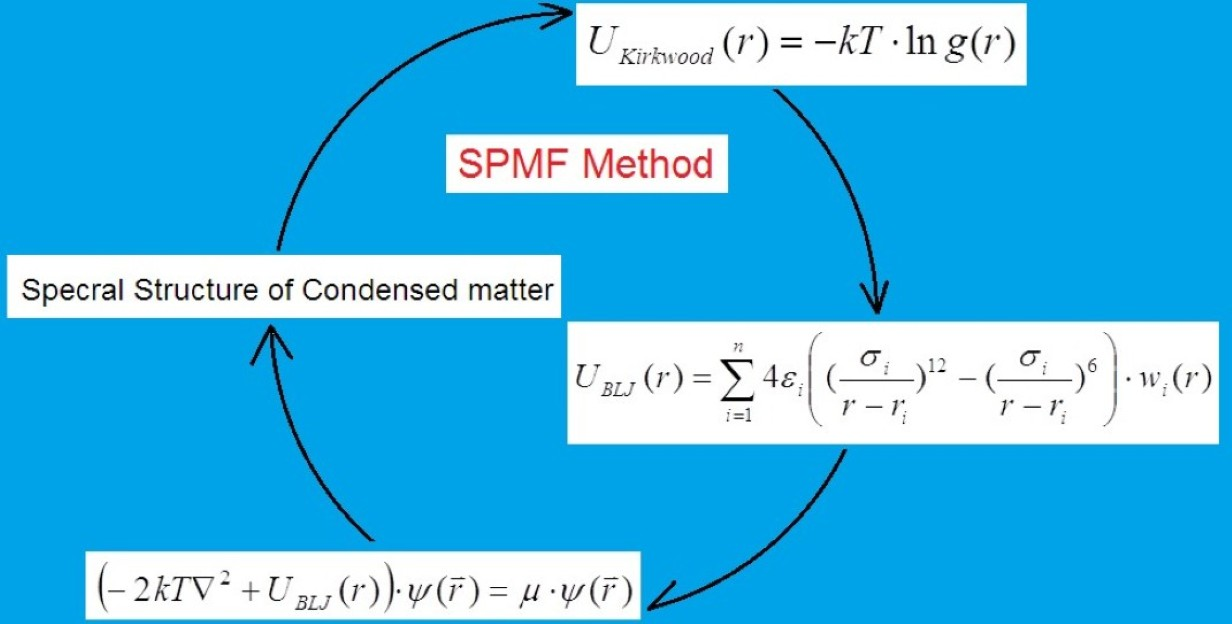
Newton’s atomistic and mechanistic vision profoundly influenced the theory of matter among 18th-century physicists and chemists. A fundamental role, although long overlooked by historiography, was played in this context by the theory of force-centers of Ruggiero Giuseppe Boscovich (1711–1787), a Dalmatian Jesuit who lived and worked for a long time in Italy. His main work, the Theoria philosophiae naturalis redacta ad unicam legem virium in natura existentium (1758–1763), represents a significant and original development of the Newtonian vision [1,2,3].

Boscovich conceives the primary elements of matter no longer as solid, extended corpuscles in the manner of Newton, but as extensionless and indivisible points, dispersed in absolute vacuum, as defined in the Theoria:

The primary elements of matter are in my opinion perfectly indivisible and non-extended points; they are so scattered in an immense vacuum that every two of them are separated from one another by a definite interval; this interval can be indefinitely increased or diminished but can never vanish altogether without compenetration of the points themselves; for I do not admit as possible any immediate contact between them.

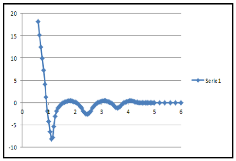
He then defines the attractive and repulsive forces by which each point interacts with every other by means the determination to approach (attraction) the negative sign of the distance variation, and with the determination to recede (repulsion) the positive sign. In this way, the sign—positive or negative—attributed to the force derives directly from the variation in distance that it tends to produce. Each point interacts according to a universal force law which, as a function of distance, presents a complex and oscillatory behavior: at sensible distances, the force becomes negligible and of gravitational type; at intermediate distances it oscillates between negative and positive values, generating a series of stable and unstable equilibrium points; at very small distances the force becomes infinitely repulsive, thus preventing the coincidence and collapse of the centers.

Boscovich’s curve stands as a unifying law for physical and chemical phenomena, offering extraordinary explanatory power. Its alternating attractive and repulsive regimes as a function of distance capture the rich diversity of condensed matter behavior: the cohesion of condensed matter arises from stable equilibria in the attractive regions of the force curve; elasticity and resistance to compression reflect the onset of repulsive interactions; while chemical affinity and the formation of molecules are accounted for by the presence of multiple equilibrium points at different distances, each corresponding to distinct stable configurations (Figure 1).

In this study, the Boscovich curve is reinterpreted as a meanfield potential for interacting particles in condensed matter: the potential, rather than accounting for local two-body interactions, may be interpreted as a global effective two-body potential that incorporates the average interactions of a generic particle with all the remaining ones. In this view, the multiplicity of its minima represents the stable states of the many-body system: the original n-body problem is thus reduced to an effective two-body problem, where geometric distances are replaced by statistical correlation distances.

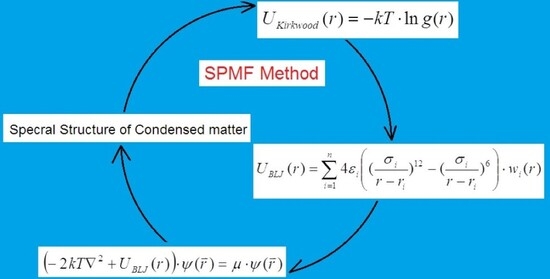
In modern terms, this reduction is achieved through a potential of mean-field, which encodes the structural information of the ensemble via the radial distribution function. The PMF exhibits multiple minima corresponding to the coordination shells, revealing the statistical structure of the system. First, starting from the radial distribution functions of packed structures—such as face-centered cubic (FCC) or hexagonal close-packed (HCP) lattices, as well as from the experimental radial distribution of liquid Argon—we have computed the multi-well PMF profiles using the Kirkwood logarithmic relation, consistently with Boscovich’s prediction. We have then developed a two-step computational procedure. In the first step, we have constructed an analytical meanfield potential by means of a weighted sum of Lennard-Jones functions, centered at the coordination distances and modulated by sigmoid curves. In the second step, we have solved the Fisher eigenvalue equation for the correlation amplitudes and reconstructed the radial distribution function as a linear combination of the squared eigenfunctions. The resulting radial distributions have been successfully compared with the expected ones.

The study of condensed matter has traditionally relied on two main theoretical frameworks: classical Density Functional Theory (cDFT) and the Ornstein–Zernike (OZ) integral equation theory. The cDFT expresses the potential as a functional of the density profile, requiring approximations for the excess free-energy functional and leading to computationally demanding Euler–Lagrange equations. The OZ approach provides an exact relation between the total and direct correlation functions but requires closure approximations that introduce systematic errors and thermodynamic inconsistencies.

In this work, we propose an alternative approach, the Spectral Potential MeanField (SPMF) method. The mean-field potential (PMF) is modeled as a weighted sum of Lennard-Jones (LJ) terms; this LJ-based PMF is first validated by comparison with the Kirkwood PMF, obtained from a known radial distribution function: this step ensures that the LJ representation correctly reproduces the structural features of the system. Then, the LJ PMF is introduced into the Fisher equation for the correlation amplitudes. The solution yields a discrete spectrum of eigenvalues and eigenfunctions, interpreted as potential levels and correlation modes associated with the coordination shells. The radial distribution function is then reconstructed as a linear combination of the squared eigenfunctions. The method is validated against structural data for liquid argon and for face-centered cubic (FCC) lattices, showing good agreement with experimental and theoretical reference data. Finally, the approach establishes a historical connection with Boscovich’s 1763 curve [1], reinterpreted here as a statistical potential, bridging eighteenth-century physics with modern statistical mechanics.

2. Boscovich’s Curve and Correlation Functions

At the basis of the statistical interpretation of Boscovich’s curve lies the theory of correlation functions [4,5]. Given a generic function f(x), consider its corresponding autocorrelation function F(r) (convolution of f with itself):

$$F(r)={\displaystyle {\int }_{-\infty }^{+\infty }f(x)}f(x+r)dx$$

which can be normalized by ${\displaystyle {\int }_{-\infty }^{+\infty }{f}^2(x)}dx$.

Consider the radial distribution function g(r); for an isotropic system, g(r) depends only on the distance. Let us define the corresponding correlation function of the number density:

$$g(r)={\displaystyle \frac{1}{{\rho }^2}}{\displaystyle \int <\rho (\overrightarrow{r}\prime )\rho (\overrightarrow{r}\prime +\overrightarrow{r})d^3\overrightarrow{r}\prime }$$

where ρ(r) is the particle density:

$$\rho (\overrightarrow{r})={\displaystyle \sum _{i=1}^N\delta (\overrightarrow{r}-{\overrightarrow{r}}_i)}$$

In compact form, introducing the density fluctuation δρ(r) = ρ(r) − ρ₀, one obtains the density correlation function:

$$C(r)={\displaystyle \int <\delta \rho (\overrightarrow{r}\prime )\cdot \delta \rho (\overrightarrow{r}\prime +\overrightarrow{r})>d^3\overrightarrow{r}\prime }$$

From which we obtain the radial distribution function:

$$g(r)=1+{\displaystyle \frac{C(r)}{\rho }}=1+{\displaystyle \frac{1}{\rho }}{\displaystyle \int <\delta \rho (\overrightarrow{r}\prime )\cdot \delta \rho (\overrightarrow{r}\prime +\overrightarrow{r})>d^3\overrightarrow{r}\prime }$$

The representation of g(r) as an autocorrelation function reflects the spatial memory of the system: the presence of a particle at r′ conditions the probability of finding another particle at r′ + r. The oscillatory shape of Boscovich’s curve—peaks and valleys—arises from the alternation of enhanced probability (g(r) > 1) and depleted probability (g(r) < 1) in the particle distribution: when g(r) = 1, the system behaves locally as an ideal gas, indicating the absence of spatial correlations. The statistical potential naturally anticipates the structure of condensed matter: its attractive minima correspond to maxima of g(r) (enhanced local density), while its repulsive maxima correspond to minima of g(r) (depleted density).

3. From cDFT and OZ Theories to the SPMF Method

The SPMF is positioned within the framework of condensed matter theory, offering an alternative approach to both cDFT) and the theory based on the OZ equation and its closures.

The cDFT is a formally exact approach for calculating the equilibrium properties of fluids [6,7]. Its fundamental principle is the expression of the grand canonical potential as a functional of the local density ρ(r), which depends on the spatial distribution of particles at each point of the system. Minimization of this functional with respect to ρ(r) yields the equilibrium density profile at fixed temperature and potential levels, allowing the calculation of all thermodynamic properties of the system. This formulation reduces the many-body problem to the determination of the density field, making it possible to treat complex systems such as interfaces, confined fluids, and nanostructured materials [7,8]. Despite its formal exactness, cDFT presents two operational challenges. The first concerns the determination of the excess free energy functional F_exc [ρ], which is not known analytically and requires approximations. The most common strategies include weighted-density approximations [9], fundamental measure theory for hard-sphere systems [10], and perturbative schemes based on expansion around a reference system [11]. The second challenge is computational: the Euler–Lagrange equations derived from functional minimization are nonlinear integrodifferential equations, whose solution often requires significant computational cost, especially for three-dimensional, dense, or long-range interacting systems [8]. Recent progress in machine learning techniques has shown significant potential for accelerating these calculations and improving functional accuracy [12,13].

The approach based on the OrnsteinZernike equation constitutes an alternative pillar for the study of the structure of condensed matter [14,15]. The exact OZ equation relates the total correlation function h(r) = g(r) − 1 to the direct correlation function c(r):

h(r) = c(r) + ρ∫c(r′)h(∣r − r′∣)dr′

The OZ equation, however, is not closed: it requires an additional relation (closure) linking c(r) to the interaction potential u(r). The most well-known closures include: Percus–Yevick method, particularly accurate for short-range interactions such as hard spheres; Hypernetted-Chain method, preferable for fluids with long-range potentials (e.g., Lennard-Jones); and the Mean Spherical Approximation method, analytically solvable for several models [7,15]. In all these closures, the bridge function b(r) is approximated or neglected, introducing systematic errors and thermodynamic inconsistencies [15]. Recently, machine learning approaches have been proposed to improve the accuracy and computational efficiency of OZ closures [13,16].

Our SPMF method differs from the approaches described above in several fundamental aspects: the Boscovich curve (1763), historically interpreted as a direct force law between two force centers, is here reinterpreted as a statistical potential of mean-field. The PMF is modeled as a weighted sum of Lennard-Jones potentials, where a sigmoid function smooths the contributions beyond the corresponding coordination shell. This representation is not an approximate closure like those of OZ, but a physically motivated parametrization of the PMF.

As a preliminary step, the LJ Boscovich mean potential is validated by comparing it with the PMF obtained from the Kirkwood equation starting from known radial distribution function (experimental or from geometric models such as FCC or HCP). Then, the potential is used in the Fisher equation for the correlation amplitudes: this eigenvalue differential equation, applied to density fluctuations in classical fluids, is here employed to obtain a discrete spectrum of eigenvalues and eigenfunctions [17]. The eigenvalues are interpreted as potential levels associated with the different coordination shells. The radial distribution function is reconstructed as a linear combination of the squared eigenfunctions. This spectral reconstruction offers a radically different perspective compared to the OZ approach, which instead solves a nonlinear integral equation to obtain the radial distribution function starting from the direct potential.

4. The Mean-Field Potential and the Radial Distribution Function

Boscovich’s curve, generally conceived as a direct interaction law between two force centers, can be interpreted as a mean potential of the entire system, which takes into account the average effect of all particles as a function of the correlation distance. In this interpretation, Boscovich’s curve would not be an elementary force law, but an emergent property of the many-body system, anticipating the modern theory of statistical thermodynamics.

Consider the PMF as defined by Kirkwood, which describes the potential of the entire system, taking into account the average effect of all particles as a function of the correlation distance [18]. In statistical thermodynamics, the PMF is defined as:

$$U_B(r)=-kT\cdot \ln g(r)$$

where k is the Boltzmann constant, T is the absolute temperature, and g(r) is the radial distribution function (pair correlation function) [14,19]. This relation shows that U_B (r) is proportional to the logarithm of the probability of finding two particles at distance r, averaged over all configurations of the system: it, therefore, represents the effective potential associated with the spatial correlation between two particles in a heat bath [7].

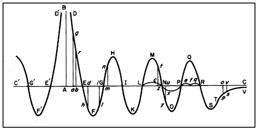
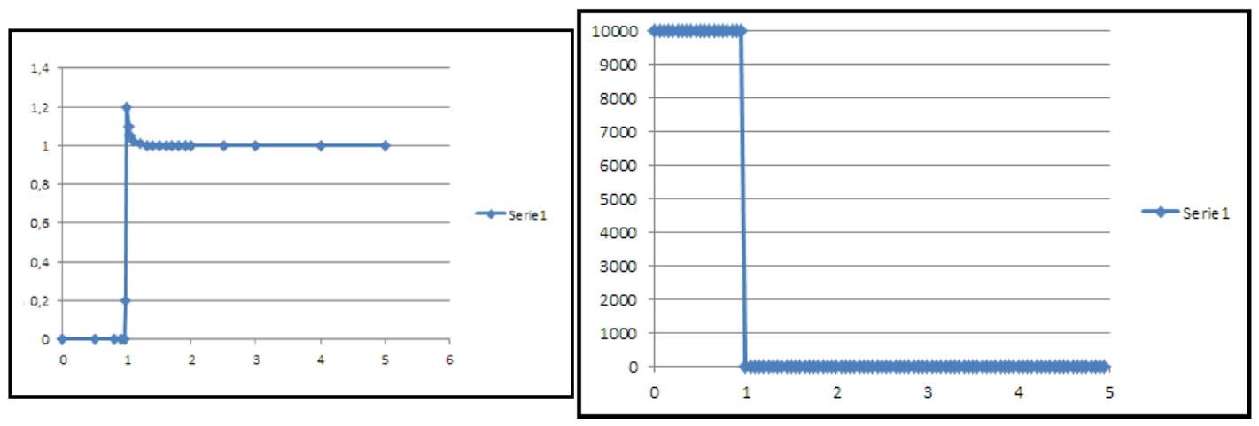
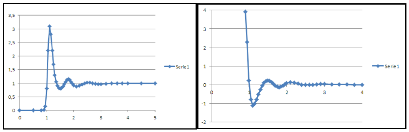
Considering gases and states of condensed matter, given the radial distribution function, we calculate the corresponding PMF. For a van der Waals gas modeled as a system of hard spheres, the interaction is zero for distances greater than the diameter σ and infinite (repulsive) for smaller distances. The radial distribution function is:

g(r) = {0 per r < σ; 1 per r ≥ σ}

The corresponding mean-field potential is:

U_B (r) = {+∞ per r < σ; 0 per r ≥ σ}

This is a step function at the contact distance: an infinitely repulsive potential at short range (impenetrability) and zero elsewhere. This case falls outside Boscovich’s framework, which requires an oscillating potential with attractive wells and repulsive barriers, and which is devoid of singularities except at the asymptotic limits. However, the van der Waals gas represents the simplest case and constitutes the starting point for more complex models (Figure 2).

For a simple liquid (e.g., a Lennard-Jones liquid), the radial distribution function exhibits a single prominent peak corresponding to the maximum packing distance (first neighbors), followed by a much weaker second peak and a rapid damping to g(r)→1as r→∞. The corresponding mean-field potential is: an attractive well (minimum) at the peak of g(r), where the potential is minimal (favorable configuration); a repulsive barrier (maximum) immediately after the first peak, corresponding to the minimum of g(r) (rarefaction zone); damped oscillations that tend to zero as r→∞.

Unlike the gas, in agreement with Boscovich’s curve, here an alternation of attraction and repulsion appears, but limited to a few oscillations. This reflects the short-range order typical of liquids: particles have a well-defined first coordination shell, but no long-range correlation (Figure 3).

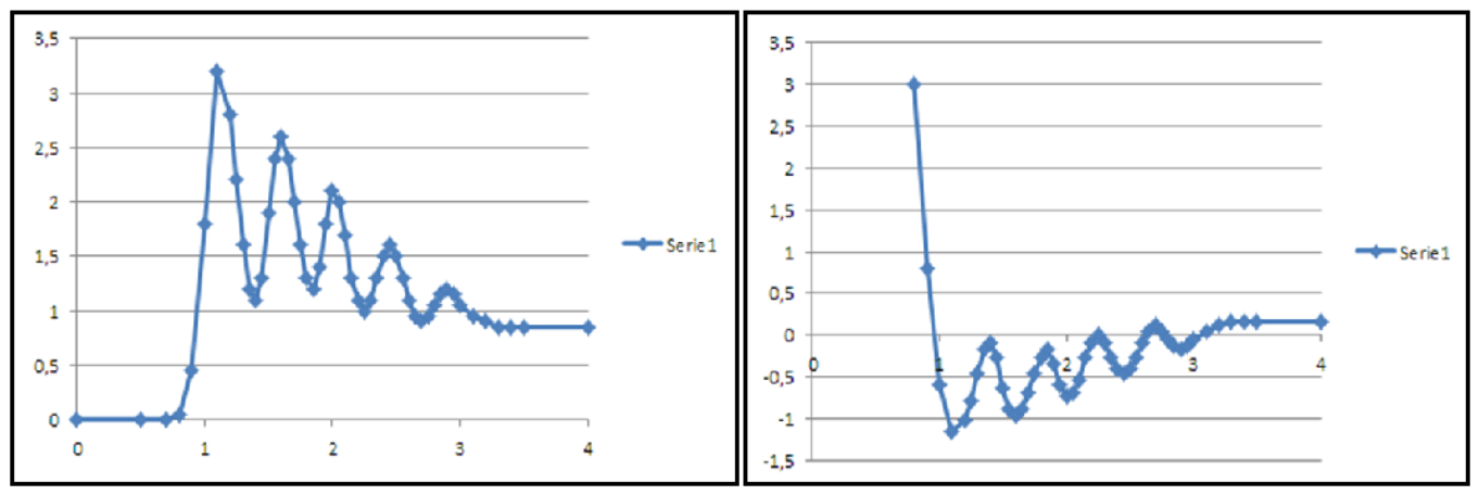
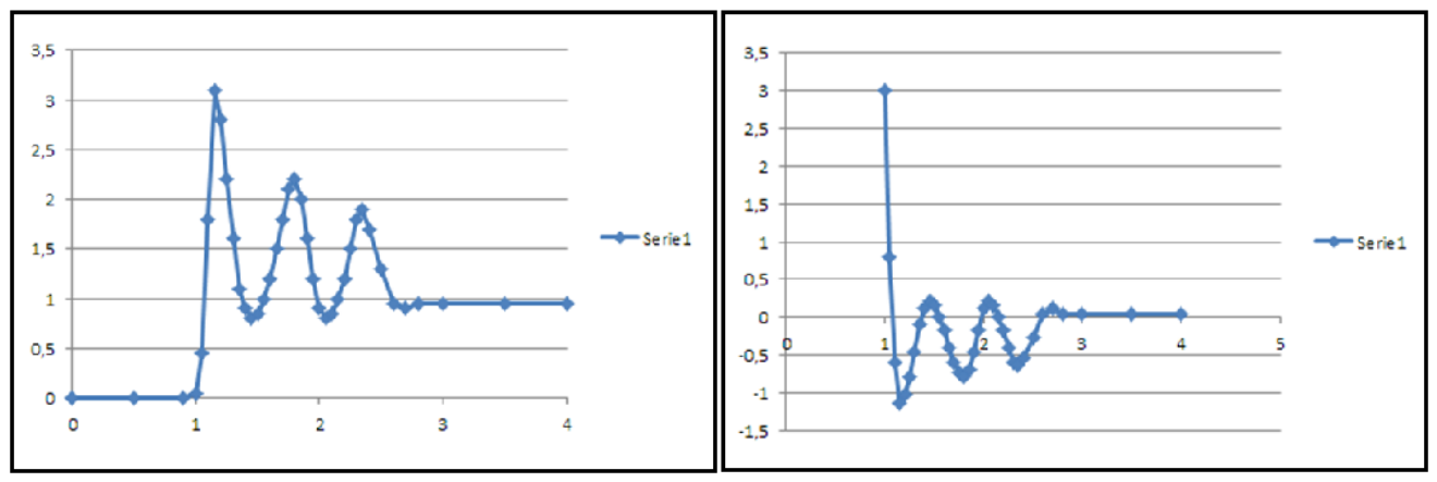
For a crystalline solid, for example, a face-centered cubic (FCC) or hexagonal close-packed (HCP) lattice, the radial distribution function exhibits a succession of well-defined and persistent peaks, corresponding to the correlation shells of the ordered structure (first, second, third neighbors, etc.) [21,22].

The corresponding PMF has a persistent oscillatory behavior: minima (attractive wells) at each peak of g(r), with depth decreasing as distance increases; maxima (repulsive barriers) at each valley of g(r), with height decreasing; and an asymptote to zero (from negative values) as r→∞, corresponding to residual attraction (van der Waals forces) and loss of correlation.

This alternation of minima and maxima is the distinctive feature of Boscovich’s curve for solids. It reflects the long-range order of the crystalline lattice: particles occupy well-defined positions, and the PMF senses all coordination shells (Figure 4 and Figure 5).

5. The PMF as Weighted Sum of Lennard-Jones Potentials

The Lennard-Jones (LJ) potential is a simple but effective model for the interaction between two neutral particles:

U_LJ (r) = 4ϵ[(σ/r)¹² − (σ/r)⁶]

It exhibits a repulsive asymptote as r→0 (due to the r⁻¹² term), a minimum at r_min=2^1/6σ of depth ϵ, and a decay to zero as r→∞.

To reproduce the oscillatory behavior of U_B (r), we model the PMF as a superposition of LJ potentials centered at different distances r_i, each representing a coordination shell. A direct superposition of LJ potentials centered at different distances would create spurious asymptotes at each r_i. To avoid this, a sigmoidal weight function is introduced, which gradually activates each potential only when the distance r exceeds a certain threshold:

$$w_i(r)={\displaystyle \frac{1}{1+e^{-k(r-r_i^{on})}}}$$

where k is the activation slope (typically k ≈ 10−15) and r_i^on is the activation distance, chosen such that r_i^on < r_i.

The PMF is thus represented as:

$$U(r)={\displaystyle \sum _{i=1}^n{w}_i(r)4{\epsilon }_i\cdot \left({(\frac{{\sigma }_i}{r-r_i})}^{12}-{(\frac{{\sigma }_i}{r-r_i})}^6\right)}$$

where r_i is the position of the minimum of the i-th potential, corresponding to the peak of g(r), and w_i (r) is the sigmoidal activation function.

For i = 1, we set r₁ = 0 and r₁^on = 0, so that the first potential is active from the beginning and provides the repulsive asymptote as r→0. For i > 1, r_i^on is chosen slightly before the minimum of the previous potential, ensuring that the new potential gradually activates after the previous peak.

The use of Lennard-Jones potentials is motivated both by their physical relevance and by their mathematical convenience. The LJ potential is the standard model for intermolecular interactions in noble gases and simple condensed phases. In a dense system, a reference particle interacts not only with its nearest neighbors, but also with particles belonging to higher coordination shells. It is, therefore, physically natural to represent the meanfield potential U_B (r) as a superposition of LJ-like contributions (PMF-LJ), each centered at the average distance of a given coordination shell, weighted by the corresponding coordination number and thermal broadening.

From a practical standpoint, the LJ representation offers the advantage of reproducing the shape of each well with a minimal number of parameters. This choice is not unique: any other set of localized functions—such as Gaussians or Morse potentials—could serve the same purpose. However, the LJ form is particularly suitable for the present case, as it encodes both the repulsive core and the attractive tail that characterize the effective interactions in condensed matter.

Figure 6 shows the PMF-LJ corresponding to the sum of five superimposed and weighted potentials.

6. Alternative Multi-Minimum Potentials

The representation of the PMF as a weighted sum of Lennard-Jones terms (LJ-PMF) is a physically motivated choice, but it is by no means unique. A variety of alternative analytical forms can be employed to model multi-minimum effective potentials, each with its own advantages and physical interpretations.

The force curve conceived by Boscovich is the result of a geometric construction that satisfies three fundamental physical requirements: the force must diverge to +∞ as x → 0, ensuring the impenetrability of bodies (1); it must tend to 0⁻ as x → ∞, reproducing Newtonian gravitational attraction (2); it must intersect the x-axis at a finite number of points (zeros), alternating between attractive and repulsive sections to explain the cohesion of matter and the formation of stable aggregates (3).

In Supplementum III to the Theoria, Boscovich translates this geometric construction into a rational analytic expression, introducing the auxiliary variable z = x² and writing the force as $y={\displaystyle \frac{P(z)}{Q(z)}}$, where P(z) is a polynomial of degree m whose positive real roots correspond to the squares of the equilibrium distances, and Q(z) is a polynomial positive for z > 0, constructed with complex conjugate roots and containing a factor z for the poles as x → 0 or x → ∞ [1,2,3].

Despite its conceptual elegance, this rational representation introduces significant numerical challenges in the SPMF method, particularly in the selection of polynomial coefficients that ensure a physically meaningful behavior while preserving the correct number and position of the minima and maxima over the entire range of distances.

For this reason, the present implementation adopts the superposition of Lennard-Jones potentials, which offers an optimal balance between physical interpretability and numerical robustness, while the Boscovich’s rational form is deferred to future developments.

The Morse potential is a widely used two-body potential that shares qualitative features with LJ but offers greater flexibility:

U_Morse (r) = E₀ [1 − exp(−k(r − r₀ ))]²

where E₀ is the well depth, r₀ is the equilibrium distance, and k controls the width of the well. The Morse potential decays exponentially rather than as r⁻⁶, making it softer at long range. A multi-minimum PMF could be constructed as a weighted sum of Morse terms:

U_B (r)= ∑_i E_i [1−exp(−k_i(r − r_i)]² ⋅S_i (r)

where each Morse well corresponds to a coordination shell. The Morse potential is widely employed to model interatomic interactions, such as those in diatomic molecules and covalent bonds. However, its use for intermolecular interactions in condensed phases—where van der Waals forces and long-range dispersion play a dominant role—is less physically motivated.

A weighted Gaussian basis provides a flexible and computationally convenient representation of localized potential wells:

U_B (r) = ∑_i G_i exp[−2σ_i ²(r − r_i )²]⋅S_i (r)

Gaussian functions have been used to approximate Morse potentials in semiclassical calculations, as demonstrated in studies of the canonical ensemble for a one-dimensional Morse system. Gaussian representations offer the advantage of analytical tractability for integrals involving the potential, making them suitable for quantum and semiclassical treatments.

A purely Gaussian sum is always positive and cannot describe attractive wells. This limitation is overcome by a signed Gaussian representation, where the amplitude of each Gaussian is modulated by a sinusoidal function, ensuring alternating signs:

U_B (r) = ∑_i A_i sin(λ_i2π(r − r_i))exp[−2σ_i² (r − r_i)²]⋅S_i(r)

This formulation naturally encodes the oscillatory structure of the PMF, with negative amplitudes corresponding to attractive wells and positive amplitudes to repulsive barriers, in agreement with Boscovich’s original curve. This simple extension preserves the analytical convenience of Gaussian functions while enabling the description of both attractive and repulsive regions of the PMF. Alternatively, one may use a difference of Gaussians or combine Gaussian terms with other functional forms to reproduce the oscillatory structure of the PMF.

Among the various possible representations of the multi-minimum PMF, the weighted sum of Lennard-Jones (LJ) terms remains the preferred choice: while alternative forms such as Boscovich, Morse, or Gaussian potentials may offer greater flexibility in specific cases, the LJ representation strikes an optimal balance between physical realism, interpretability, and numerical convenience, which justifies its adoption in the present work.

7. The Fisher Density Functional Equation

We introduce the correlation amplitude $\psi (r)=\sqrt{g(r)}$: since g(r) ≥ 0, ψ(r) is real and non-negative. The relationship with the PMF is:

U_B (r) = −k Tlng(r) = −2k Tlnψ(r)

Within the framework of classical Density Functional Theory, in the mean-field approximation, it can be shown that ψ(r) satisfies the Fisher equation for the correlation amplitudes:

−2kT ∇²ψ(r) + U_B (r)ψ(r) = μψ(r)

where ψ_i (r) are the correlation amplitudes (eigenfunctions), μ_i are the potential levels (eigenvalues), and U_B (r) is the PMF. The radial distribution function is then obtained as a linear combination of the squares of the correlation amplitudes. The Fisher equation is well known in the theory of classical fluids and arises from the linearization of the density functional theory (DFT) for non-uniform fluids. It describes the spectrum of density fluctuations around a uniform mean density and is routinely used in the study of liquid structure and the liquid–solid interface [6,14].

Since U_B (r) has a series of minima (wells) separated by maxima (barriers), the spectrum consists of eigenvalues μ₁, μ₂, μ₃, … corresponding to the ground states of the wells, and the eigenfunctions ψ_i(r) describe the spatial correlation amplitude for each mode. The corresponding radial distribution function is:

g_i(r) = ψ_i (r)²

For a state localized in the i-th well, ψ_i(r) has a maximum at the minimum of U_B(r) a r= r_i.

The total radial distribution function g(r) is expanded in the basis of the eigenfunctions ψ_i (r) as:

g(r) = ∑_i c_i ψ_i (r)²

where the coefficients c_i represent the statistical weights (e.g., Boltzmann weights) associated with each eigenstate. The peaks of g(r) correspond to the maxima of the eigenfunctions in the wells.

To solve the problem numerically, we consider U_B (r) as a weighted sum of Lennard-Jones potentials with appropriate parameters (adapted to the material structure, e.g., FCC) (1); we impose the boundary conditions ψ(0) = 0 and ψ(r)→1 as r→∞ (2); we solve the eigenvalue problem, obtaining the eigenvalues μ₁, μ₂, μ₃,… and the eigenfunctions ψ₁ (r), ψ₂ (r), ψ₃ (r), … (3); we compute g_i(r) = ψ_i(r)² (4). The peaks of g(r) (statistical shells) correspond to the eigenfunctions localized at the minima of U_B (r). The radial distribution function is obtained as g(r) = ψ(r)², where ψ(r) is the linear combination of eigenfunctions weighted by the thermal occupation coefficients. The calculated values are then compared with the expected g(r) for the system under study (5). The peaks of g(r) (statistical shells) correspond to the eigenfunctions localized at the minima of the potential.

Starting from the statistical hypothesis underlying Boscovich’s curve, this approach provides a formal bridge between statistical mechanics and spectral theory. The shell structure observed in the states of aggregation of matter is interpreted as a result of a discrete eigenvalue spectrum arising from a classical density functional equation for the correlation amplitudes.

8. The Mean-Field Potential for an FCC Lattice

The objective of this numerical calculation is to solve the classical Fisher equation for the correlation amplitude $\psi (r)=\sqrt{g(r)}$, where g(r) is the radial distribution function of a system of interacting particles. The effective potential appearing in the equation is the mean-field potential U_B (r), which we model as a weighted sum of Lennard-Jones potentials centered at different distances, corresponding to the coordination shells of a face-centered cubic lattice.

In spherical symmetry, the Fisher equation reduces to the second-order ordinary differential equation:

$$-2kT{\displaystyle \frac{d^{2}u}{d{r}^2}}+U_B(r)\cdot u(r)=\mu \cdot u(r)$$

where u(r) = rψ(r) and the boundary conditions are u(0) = 0 (impenetrability) and u(r)→0 as r→∞ (bound states in the potential wells).

The parameters used for the FCC lattice are reported in

Table 1. Parameters of the mean-field potential U_B (r), modeled as a weighted sum of five Lennard-Jones potentials, employed in the face-centered cubic (FCC) lattice model. The parameters—well depths, widths, and coordination distances—are assigned on the basis of the known structural properties of the FCC lattice (see text for details).

i	ri	εi	δi	ri on	k
1	1.10	5.0	0.30	1.00	15
2	1.60	3.0	0.35	1.50	15
3	2.00	2.0	0.40	1.90	15
4	2.40	1.2	0.45	2.30	15
5	2.80	0.8	0.50	2.70	15

. The distances r_i correspond to the first five coordination shells of the FCC lattice (in reduced units where the first peak is at 1.10). The depths ϵ_i are chosen to decrease with i, and the widths σ_i increase to simulate the broadening of the peaks at large distances. The activation thresholds r_i^on are set just before the minimum of the previous potential, as described previously.

Our approach does not rely on a fitting procedure to adjust the Lennard-Jones parameters to reference data. Instead, the parameters are assigned on physical grounds, using the peak positions of the Kirkwood potential of mean-field derived from the input g(r). In other words, the LJ potential is not optimized to reproduce the data. The goal of this work is not to achieve the best possible fit to reference data, but to demonstrate that—with a physically motivated choice of the parameters—the SPMF method is capable of correctly reproducing the essential structural features of the system. While the parameters have been chosen on physical grounds, we acknowledge that the method could be extended to include an optimization procedure, should a more quantitative agreement be desired.

The first five eigenvalues obtained from the calculation are listed in

Table 2. Eigenvalues obtained for the face-centered cubic (FCC) lattice model. See text for details.

i	µi	Ground State
1	–4.82	1st well
2	–2.93	2nd well
3	–1.87	3rd well
4	–1.05	4th well
5	–0.52	5th well

. Each eigenvalue represents the ground-state energy of a different well in the multi-well potential.

The eigenvalues μ_i are negative and decrease in magnitude with increasing shell index, implying that the coordination wells become progressively shallower. This behavior is consistent with the attenuation of the peaks of g(r) at larger distances, and with the progressive loss of spatial correlation in the system.

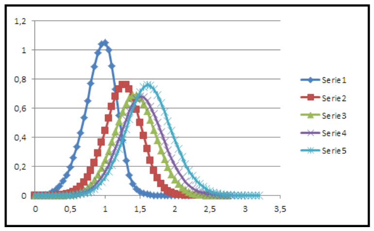
The eigenfunctions ${\psi }_i(r)={\displaystyle \frac{u_i(r)}{r}}$ have been calculated and normalized such that ${\displaystyle {\displaystyle \underset{0}{\overset{\infty }{\int }}}{\psi }_i{(r)}^{2}4\pi r^{2}dr=1}$. They exhibit a localized maximum at the potential minimum (Figure 7).

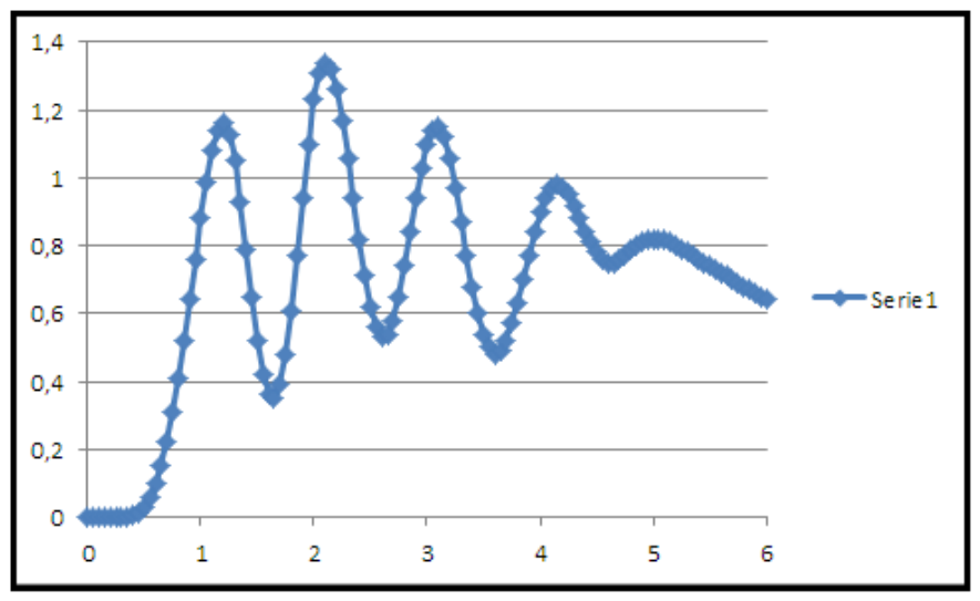
The total radial distribution function in Figure 8 was calculated as:

$$g(r)={\displaystyle \sum _{i=1}^5}{c}_i{\psi }_i{(r)}^2$$

where the coefficients c_i were chosen to reproduce the relative peak heights expected for the FCC lattice, shown in Figure 3 (

Table 3. Coefficients c_i of the linear combination for the radial distribution function g(r) in the FCC model. See text for details.

i	ci
1	1.00
2	0.85
3	0.70
4	0.50
5	0.30

).

In conclusion, the numerical procedure has enabled us to: (1) construct the mean-field potential UB (r) as a weighted sum of Lennard-Jones potentials centered at the coordination shell distances of the FCC lattice; (2) solve the associated classical eigenvalue problem, yielding negative eigenvalues μi and eigenfunctions ψi (r) localized within the corresponding potential wells; and (3) reconstruct the radial distribution function g(r), which correctly reproduces the expected peak positions for the FCC structure.

The method shows that, starting from Boscovich’s curve interpreted as a mean-field potential, it is possible to describe the shell structure of condensed matter. The formulation as an eigenvalue problem provides a rigorous mathematical basis for calculating correlation properties. The accuracy of the calculation can be improved by optimizing the potential parameters to better fit the expected structure, and by including a larger number of eigenfunctions.

9. The SPMF for a Liquid

We apply the mean potential model to liquid argon at 85 K. Liquid argon is a classic example of a simple Lennard-Jones liquid, with a radial distribution function g(r) extensively studied experimentally by neutron and X-ray diffraction [20].

The procedure is conceptually identical for both the FCC lattice and the liquid, and consists of the following common steps. First, the Kirkwood potential of mean-field is obtained from the radial distribution function g(r). The input g(r) may be either the ideal function for the FCC lattice (theoretically computed) or the experimental one for liquid argon. Second, the Kirkwood PMF is modeled by a weighted sum of Lennard-Jones potentials, centered at the coordination distances and modulated by sigmoid functions. Third, the resulting LJ potential is inserted into the Fisher equation for the correlation amplitudes, yielding a discrete spectrum of eigenvalues and eigenfunctions. Finally, the radial distribution function is reconstructed as a linear combination of the squared eigenfunctions and compared with the input g(r).

The only difference between the two cases lies in the nature of the input g(r). For the FCC lattice, g(r) consists of sharp, well-defined peaks at the characteristic coordination distances. For the liquid, g(r) is a broader and more damped function, reflecting thermal motion and structural disorder. As a consequence, the resulting Kirkwood PMF exhibits deeper and narrower wells for the FCC lattice, and shallower, wider wells for the liquid. Nevertheless, the parametrization via LJ terms and the subsequent solution of the Fisher equation remain unchanged.

The eigenvalue problem is discretized on a radial grid and solved numerically using the finite difference method. The eigenvalues μ_i correspond to the potential levels associated with different coordination shells, while the eigenfunctions ψ_i(r) represent the correlation amplitudes. 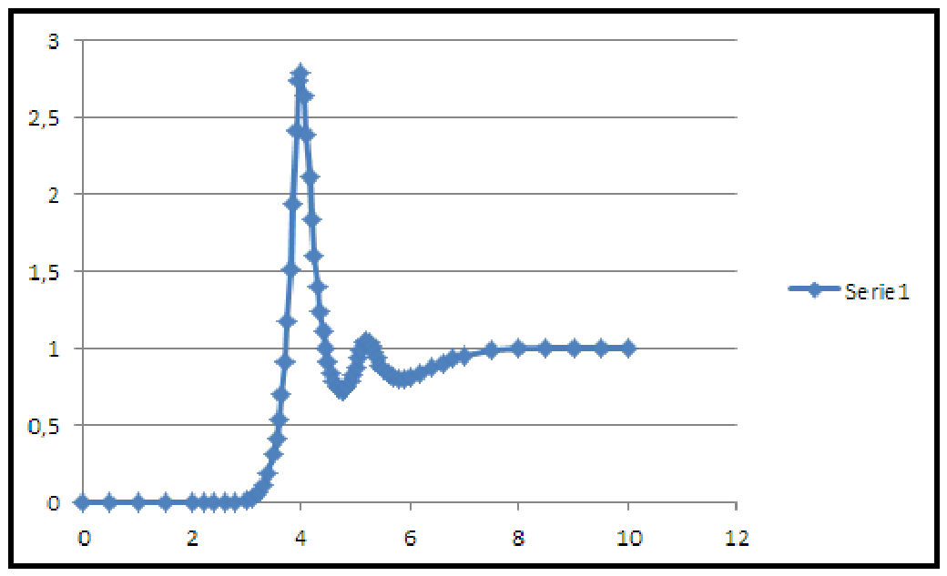The radial distribution function is obtained as a linear combination of the squares of the eigenfunctions g(r) = ∑ _i c_i ψ_i (r)², where the coefficients c_i are chosen to reproduce the experimental data shown in Figure 6. The calculation reproduces the main features of the experimental g(r) for liquid argon: a pronounced first peak at r ≈ 3.75 Å, a first minimum at r ≈ 4.5 Å, and a much lower second peak at r ≈ 5.2 Å, in agreement with the experimental data of Yarnell et al. (1973) [20] (Figure 9).

10. Perspectives

The procedure presented in this work is a non-self-consistent approach. However, the method can be naturally extended to a self-consistent scheme (SC-SPMF), in which the coordination shell positions emerge iteratively from the calculation itself. The conceptual framework is as follows:

Initial guess: a starting PMF is constructed, for example, as a sum of Lennard-Jones terms centered at estimated coordination distances (1); Fisher step: the Fisher equation is solved with this PMF, yielding a discrete spectrum of eigenvalues, eigenfunctions, and the radial distribution function is reconstructed as a linear combination of the squared eigenfunctions (2); Kirkwood step: a new PMF is obtained from the reconstructed g(r) using the Kirkwood relation (3); iteration, i.e., until the changes in the PMF and in the coordination distances fall below a chosen tolerance (4). The coordination shell distances are emergent outputs of the calculation, determined by the self-consistent interplay between structure and effective potential.

Despite its conceptual appeal and promising potential, the implementation of the self-consistent SPMF method is beyond the scope of the present work. It introduces several numerical challenges, including: the choice of an appropriate basis for the PMF parametrization during the iteration (1); the need to ensure stability and avoid divergence in the Kirkwood step (2); the dependence of the convergence on the initial guess and on the temperature.

The conceptual framework of the SPMF method is not limited to classical condensed matter. Its formal structure—an eigenvalue problem with an effective potential derived from a correlation function—suggests a natural extension to quantum mechanical systems, particularly to the mean-field description of polyelectronic atoms.

In the present classical formulation, the Fisher equation plays the role of an effective Schrödinger equation for the correlation amplitudes. The potential U_B (r) is not the bare interaction potential, but a mean-field potential derived from the spatial correlations of the system.

A formal analogy can be drawn with the Hartree–Fock or Kohn–Sham equations for polyelectronic atoms. In both cases: an effective potential replaces the full many-body interaction (1); the potential depends on the solution itself (through the density or the correlation function) (2); The equations must be solved self-consistently (3).

The implementation of a self-consistent quantum SPMF method presents several formidable challenges: definition of the correlation function (1), exchange and correlation: effects (2) and computational cost (3). The calculation of the electron–electron correlation function and its use in the effective potential introduces an additional computational layer compared to standard DFT.

The present work has introduced the SPMF method and validated it on spherically symmetric Lennard-Jones systems, both in the fluid and in the solid (FCC) phase. While this choice has allowed us to establish the foundational elements of the method and to test its performance against well-known reference data, the approach is by no means limited to monatomic systems with spherical interactions. A natural extension concerns molecular fluids, where the interaction potential depends not only on the distance between molecular centers but also on their relative orientation. In such systems, the radial distribution function g(r) is replaced by a set of partial correlation functions, each describing the distribution of a specific pair of molecular sites (e.g., site–site radial distribution functions). Then, the Kirkwood relation can be generalized to each partial correlation function, yielding an effective orientationally averaged PMF for each site–site pair. The Fisher equation would then be solved for each partial PMF, and the total structure could be reconstructed as a combination of the corresponding spectral modes. This approach would be particularly suitable for simple molecular fluids such as nitrogen, methane, or water, where site–site correlation functions are well characterized both experimentally and computationally.

11. Conclusions

The hypothesis that Boscovich’s curve represents a mean potential, rather than a direct two-body interaction law, is suggested first of all by a consideration of mathematical simplicity: in a direct potential, the multiplicity of minima and maxima would be unnecessary in describing the multiplicity of stable states of a many-body system. For this purpose, a single-well potential, capable of reproducing the criteria of short-range non-overlap and long-range non-interaction, would indeed suffice. Conversely, the approach may be interpreted as a reduction of the full n-body problem to an effective two-body potential with multiple minima, depending on the mean distance. It is obvious that Boscovich did not know the theory of correlation functions of complex systems; nevertheless, he could intuit its statistical significance for the description of matter.

Then, we have developed a model of the structural order of condensed matter based on a classical mean-field equation. In this equation, the multi-stage mean potential is simulated by a sum of appropriately weighted Lennard-Jones potentials.

The radial distribution function is used to extract the PMF via the Kirkwood relation, and the parameters of the LJ representation are assigned on physical grounds, without optimization against the target g(r). The reconstruction of g(r) from the Fisher eigenfunctions is, therefore, a validation test. Moreover, the Fisher equation provides additional information—potential levels and spectral fingerprints of the coordination shell structure—that is not contained in the original g(r).

Thus, the eigenvalues μ_i, corresponding to the potential levels, and the eigenfunctions ψ_i (r), interpreted as correlation amplitudes associated with the coordination shells of first, second, … neighbors, have been determined for both crystalline and liquid states. The radial distribution function was then obtained as a linear combination of the squares of these amplitudes, and the result was successfully compared with reference radial functions.

Finally, in light of the proposed hypotheses and the obtained results, the historical and epistemological reinterpretation of Boscovich’s Theoria is substantiated.