Refined Langmuir–Hinshelwood Kinetics for Heterogeneous Photocatalytic Systems: Analytical Closed-Form Solution, Enhanced Approximations and Experimental Validation

Abstract

This study takes a further step forward in the analytical treatment of Langmuir–Hinshelwood (LH) kinetics for heterogeneous catalysis by deriving its closed-form solution. Unlike previous studies, we present a general solution that does not impose severe restrictions on the experimental conditions. This solution not only recovers the typical first- and zeroth-order regimes but also enables the simultaneous determination of the reaction rate constant and absorption–desorption equilibrium constant, unlike the traditional approaches to this equation, which needed additional isotherm experiments. The final solution requires a fine mathematical treatment for its numerical implementation, but enhanced approximations of the closed-form solution overcome this problem without losing the main advantage of calculating both constants at the same time. A parameter called “critical time” has been introduced, whose calculation allows us to distinguish quantitatively between kinetic regimes. Finally, the validation of these approximations has been carried out with experiments on zinc oxide and anatase (TiO₂) under different conditions. Anatase experiments undoubtedly show a first-order tendency, regardless the quantity of powder. On the other hand, the degradation regime of the ZnO case cannot be easily ascribed to the zeroth or first order by simple inspection, but the model can mathematically rule out the zeroth order and confirm that it undergoes first-order degradation.

1. Introduction

Increasing contamination of water is one of the most pressing environmental challenges. The development of the industrial, pharmaceutical and textile industries generates wastewater containing dyes, pesticides and other persistent organic pollutants that are hazardous for human life [1,2]. Traditional wastewater treatment methods, such as chemical treatment, filtration or bio-treatment, are becoming ineffective in removing persistent organic pollutants [3]. In this context, the advanced oxidation processes, whose degradation mechanism of persistent organic pollutants relies on the generation of radical oxidating species (ROS), seems to be a promising field [4]. Among them, photocatalysis has been postulated as a natural candidate for this environmental problem due to its low cost, the chemical stability of the main catalysts and the capability of complete degradation of the polluted water [1,5].

Photocatalysis can be distinguished depending on the mode of generating electron–hole pairs: by ultraviolet light (UV photocatalysis) or visible light (visible photocatalysis). This distinction is usually made with regard to the experimental method and its results, since UV photocatalysis is more effective than visible photocatalysis [1]. Nevertheless, visible photocatalysis has become more acceptance since visible light is directly available from the sun and hence more eco-friendly [6]. In both cases, the underlying physical mechanisms are the same, and as long as the photon energy is high enough to overcome the band gap, independent of the photon source.

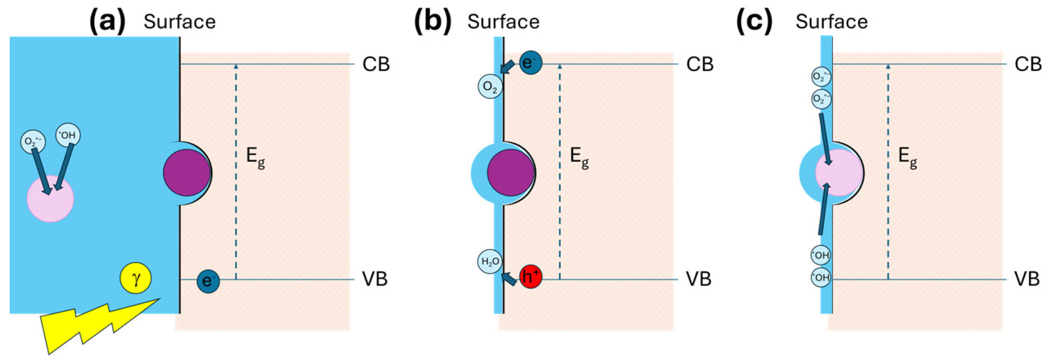
The fundamentals of photocatalysis are based on concepts that involve solid state physics and surface physics. For the sake of explanation, let us assume it to be in UV photocatalysis, and assume also that a solid semiconductor catalyst is submerged in a liquid phase with a dissolved pollutant. In this case, the semiconductor is irradiated with light whose wavelength is greater than the bandgap energy and, therefore, electrons from the valence band are promoted to the conduction band, which involves creating electron–hole pairs. Such pairs migrate to the surface of the catalyst and can react with adsorbed water molecules or dissolved gaseous oxygen to generate ROS, which will in turn react with the adsorbed pollutant and will degrade it into non-pollutant species. It is important to consider that the process of photocatalysis takes place on the surface of the catalyst all the time, and this is the reason why so much effort is made to increase the effective surface of the catalysts [7,8,9,10]. More specifically, the chemical reactions taking place in the process, following Houas et al. [11], are as follows:

• Absorption of photons by the catalyst: $\left(\mathrm{C}\mathrm{a}\mathrm{t}\mathrm{a}\mathrm{l}\mathrm{y}\mathrm{s}\mathrm{t}\right)+\mathrm{h}\mathsf{\nu }\to {\mathrm{e}}_{\mathrm{C}\mathrm{B}}^{-}+{\mathrm{h}}_{\mathrm{V}\mathrm{B}}^{+}$
• Oxygen ionosorption: ${\left({\mathrm{O}}_2\right)}_{\mathrm{a}\mathrm{d}\mathrm{s}}+{\mathrm{e}}_{\mathrm{C}\mathrm{B}}^{-}\to {\mathrm{O}}_2^{·-}$
• Neutralization of OH⁻ groups by photoholes: ${\left({\mathrm{H}}_2\mathrm{O}⟺{\mathrm{H}}^{+}+\mathrm{O}{\mathrm{H}}^{-}\right)}_{\mathrm{a}\mathrm{d}\mathrm{s}}\to {\mathrm{H}}^{+}+\mathrm{O}\mathrm{H}$
• Neutralization of ${\mathrm{O}}_2^{°-}$ by protons: ${\mathrm{O}}_2^{°-}+{\mathrm{H}}^{+}\to \mathrm{H}{\mathrm{O}}_2^{°}$
• Hydrogen peroxide formation and dismutation of oxygen: $2\mathrm{H}{\mathrm{O}}_2^{°-}\to {\mathrm{H}}_2{\mathrm{O}}_2+{\mathrm{O}}_2$
• Decomposition of hydrogen peroxide: ${\mathrm{H}}_2{\mathrm{O}}_2+{\mathrm{e}}^{-}\to \mathrm{O}{\mathrm{H}}^{°}+\mathrm{O}{\mathrm{H}}^{-}$
• Oxidation of organic reactants (R) by OH radicals: $\mathrm{R}+\mathrm{O}{\mathrm{H}}^{°}\to {\mathrm{R}}_{.}^{\prime }+{\mathrm{H}}_2\mathrm{O}$
• Direct oxidation by reaction with holes: $\mathrm{R}+{\mathrm{h}}^{+}\to {\mathrm{R}}^{+°}\to \mathrm{d}\mathrm{e}\mathrm{g}\mathrm{r}\mathrm{a}\mathrm{d}\mathrm{a}\mathrm{d}\mathrm{a}\mathrm{t}\mathrm{i}\mathrm{o}\mathrm{n} \mathrm{p}\mathrm{r}\mathrm{o}\mathrm{d}\mathrm{u}\mathrm{c}\mathrm{t}\mathrm{s}$

Figure 1 depicts a basic scheme of this mechanism, which is, essentially, steps 1 (Figure 1a), 2, 3 (Figure 1b), 7 and 8 (Figure 1c).

Theoretical photocatalysis studies began with gas–solid adsorption studies by Langmuir, which settled the bases for current theories [12,13]. Later, many theoretical studies of photocatalysis have focused on the mechanisms governing this process, which yields the formulation of several models, the Langmuir–Hinshelwood (LH) equation being the most used among them to describe the experiments [14,15]. However, the mathematical treatment of this equation has often been relegated to a second plane, due to its complexity and the subsequent difficulty finding a closed solution. In previous works [15,16], different approximations have been developed to determine the different kinetical parameters; however, the conditions for these approximations to be valid are quite restrictive. In this complex context, most experimental works implicitly assume that the limiting step in the process is the reaction of the adsorbed species, and the concentration of adsorbed species is low. With these hypotheses, the approximate solution of the LH equation yields a first-order kinetics. However, verifying the validity of the hypothesis is mathematically complex and cumbersome.

In this work, we have made a detailed study of the mathematical description of the Langmuir–Hinshelwood equation, and we have been able to find a closed solution for it. From this solution, some numerical parameters which can act as indicators for identifying the custom regimes in terms of the experiment conditions have been derived, without the need of complex mathematical treatment. It is then a sort of discriminating tool that lets us easily decide which is the optimum approximation for the experimental conditions under study.

To test the validity of the proposed theoretical treatment, several experiments have been performed. Section 2 of the paper details the experimental conditions used for the experiments that will be described in Section 4. Section 3 is devoted to the theoretical model. First, a summary of the LH approximations is given to establish the general context; then, the solution of the Lambert equation will be addressed.

2. Experimental Method

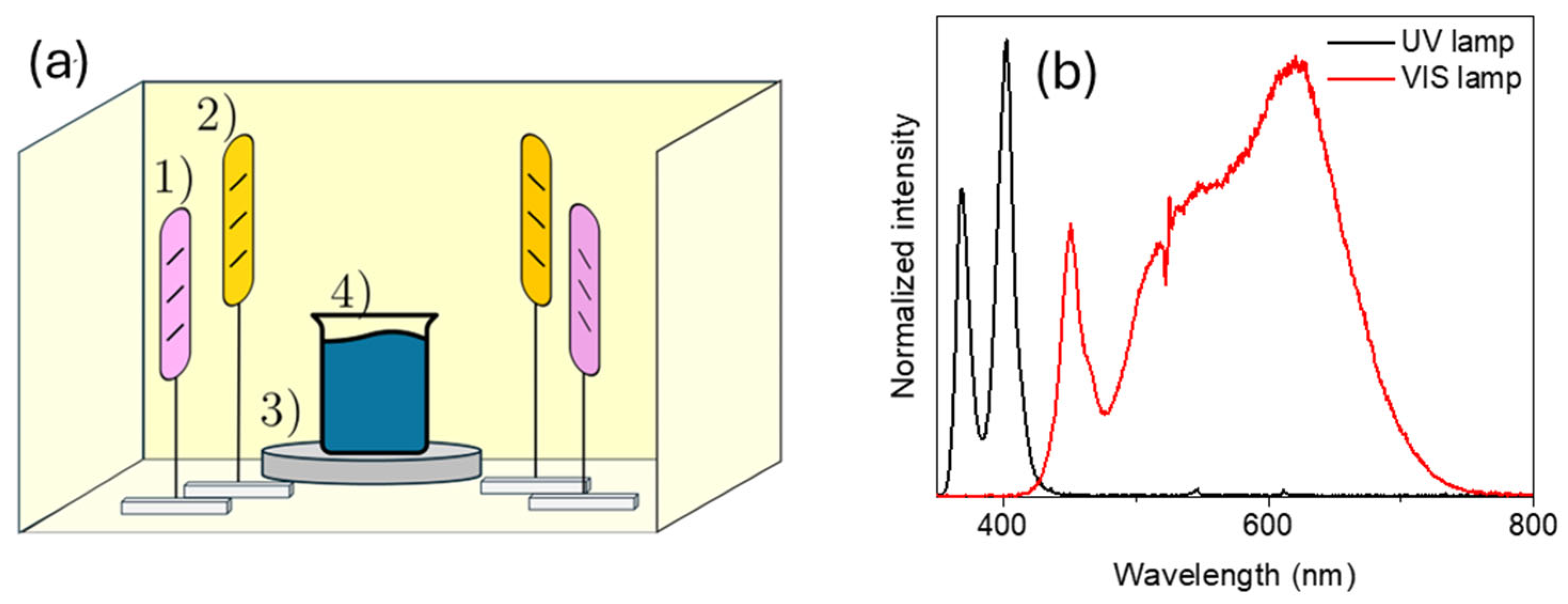
To check the validity of the analytical model, commercial powder samples of anatase (Aldrich Chemical Company (St. Louis, MO, USA), 1317-70-0) and zinc oxide (Sigma-Aldrich (St. Louis, MO, USA), #MKCL7155) have been used as catalysts, which are known for their good photocatalytic properties [17,18], and whose bandgap is around 3.2 eV at room temperature [19,20]. Commercial powder was directly added to the final solution, stirred by the vibrating plate, and aliquots were taken from the flask at different time intervals for each material. We used methylene blue (SigmaAldrich, CAS 122965-43-9) as pollutant. The photocatalysis reactor was homemade, open to air, and equipped with two commercial visible LED lamps (Brookes lamp (Grow The Jungle, Madrid, Spain), P = 35 W each one) and two commercial UV LED lamps (Mantis lamp (Grow The Jungle, Madrid, Spain), P = 25 W each one). Each UV lamp provides an illuminance of 4.5 mW/cm² at the position of the flask and each visible one provides 14 mW/cm². A simple scheme of the reactor is shown in Figure 2a. The dissolution is placed in the middle of the reactor, on top of the magnetic stirrer. The UV and visible lamps are placed around the dissolution, each one pointing at the centre in a straight line. Both lamps, whose normalized spectra are shown in Figure 2b, were used together during all the time in all experiments.

The test solutions used in this work are prepared from a parent solution of 10 mg of methylene blue (MB) in 100 mL of distilled water, having 100 ppm in volume (stock solution). Then, two different sets of experiments were performed. For the first one, we diluted 12.5 mL of stock solution into 500 mL of distilled water. This dissolution will have 2.5 ppm in volume (daughter solution) and will be tested with 2.5 mg of anatase or ZnO. For the second, we distilled 250 mL of this latter solution into 500 mL to decrease the concentration to half of the initial. This solution, having 1.25 ppm in volume (granddaughter solution), will be tested with 1.25 mg of anatase or ZnO.

Table 1. Experimental details of the experiments performed.

Number of Experiment	Element	Mass of Catalyst	Concentration of Dissolution
#1	Anatase	2.5 mg	2.5 ppm in volume
#2	Anatase	1.25 mg	1.25 ppm in volume
#3	ZnO	2.5 mg	2.5 ppm in volume
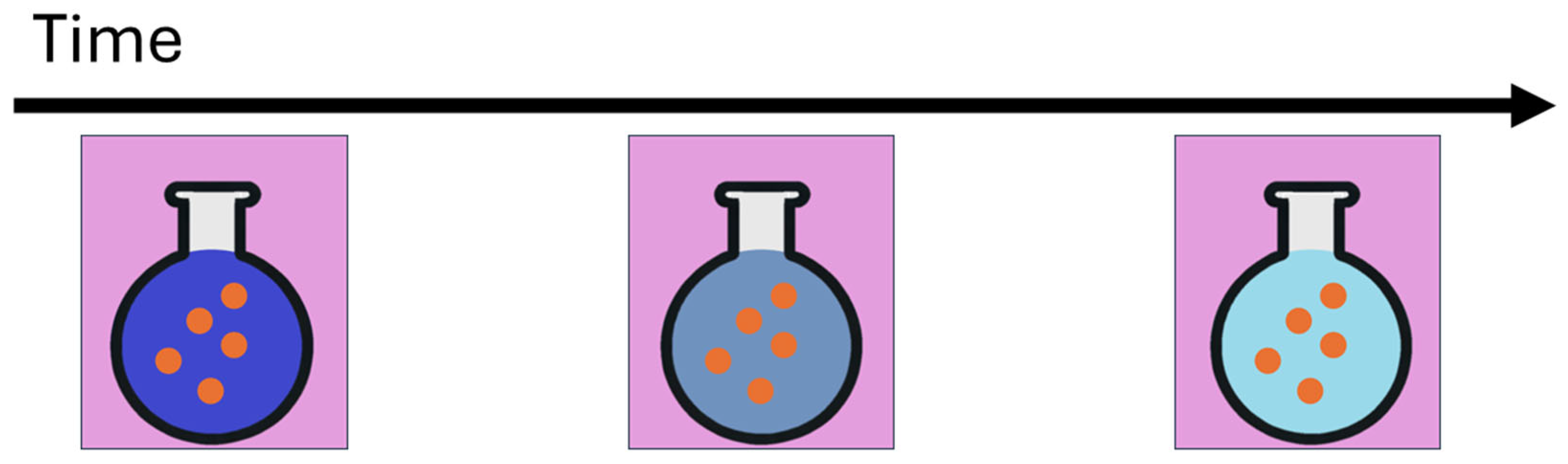
#4	ZnO	1.25 mg	1.25 ppm in volume

shows the sets used to check the validity of the model and assigns a number to each experiment to ease the discussion of results. A control experiment with MB dissolution and no samples under UV and visible light was also made to discard the influence of photolysis. To monitor the degradation, one aliquot was taken out from the reactor at different time intervals. Figure 3 illustrates these procedures. In all experiments, the dissolution with catalysts was stirred for 30 min in darkness to achieve the absorption/desorption equilibrium, and was then magnetically stirred during all the irradiation time and irradiated under UV and visible light. The absorption spectra of the aliquots were performed with a Jasco V-770 spectrometer. Finally, the fittings were calculated with Matlab 2020a Optimization Toolbox.

3. Theoretical Study

The most common kinetic model used for the degradation of organic pollutants is the Langmuir–Hinshelwood equation (LH equation). This model describes the evolution of concentration of pollutants with time, $C\left(t\right)$ (mg L⁻¹), in terms of a differential equation [16]:

$$C^{\prime }\left(t\right)=-{\displaystyle \frac{k_r{K}_{e}C\left(t\right)}{1+K_{e}C\left(t\right)}}$$

(1)

In short, the starting point for simple decomposition reactions is

$$A+S\leftrightharpoons AS\to \mathrm{F}\mathrm{i}\mathrm{n}\mathrm{a}\mathrm{l} \mathrm{p}\mathrm{r}\mathrm{o}\mathrm{d}\mathrm{u}\mathrm{c}\mathrm{t}\mathrm{s},$$

where A refers to the reactant and S to the active adsorption sites on the catalyst surface. Although the form of the reaction will depend on the process, at least one step is controlled by the adsorption on active sites.

Let us consider the simple reaction mentioned above in further detail. The catalytic reaction may be separated in three different reactions, each with its characteristic equilibrium constant, $k_1$ for adsorption, $k_{-1}$ for desorption and $k_r$ for the reaction that we want to activate. The ratio $k_r$ is always positive, since it is defined as a quotient of powers of concentrations. The global reaction rate r may be written as

$$r=k_r{C}_{AS}=k_r\theta C_s$$

(2)

where $C_A$: Concentration of adsorbate (mol/m³); $C_{AS}$: Surface concentration of occupied sites (mol/m²); $C_S$: Surface concentration of total sites (occupied by adsorbate or not) (mol/m²); and $\theta$: Surface coverage; fraction of occupied sites ${\displaystyle \frac{C_{AS}}{C_S}}$. We have already mentioned the influence of the surface, according to this model, which can be quantified through $C_S$.

When the steady state is reached

$${\displaystyle \frac{d{C}_{AS}}{dt}}=0$$

(3)

Then

$$k_1{C}_A{C}_S-k_1{C}_A{C}_{AS}-k_r{C}_{AS}-k_{-1}{C}_{AS}=0$$

(4)

where the different terms refer to the different processes taking place: $k_1{C}_A{C}_S$, adsorption of adsorbates onto all sites;$k_1{C}_A{C}_{AS}$, adsorption taking account that only empty sites are available for adsorption; $k_r{C}_{AS}$, reaction between adsorbate and sites; and $k_{-1}{C}_{AS}$, desorption.

In terms of coverage $\theta ={\displaystyle \frac{C_{AS}}{C_S}}$, we can rewrite the equation as

$$k_1{C}_A{C}_S\left(1-\theta \right)-k_r\theta C_S-k_{-1}\theta C_S=0,$$

(5)

and

$$\theta ={\displaystyle \frac{k_1{C}_A}{k_1{C}_A+k_{-1}+k_r}}$$

(6)

Considering that in steady state $r=k_r\theta C_s$

$$r={\displaystyle \frac{k_1{k_{r}C}_A{C}_S}{k_1{C}_A+k_{-1}+k_r}}$$

(7)

Now we can describe two scenarios in terms of the limiting step.

If the limiting step is the adsorption

$$k_r\gg k_1{C}_A; k_{-1}\Rrightarrow r\approx k_1{C}_A{C}_S$$

(8)

If the limiting step is the reaction of adsorbed species, and setting $K_e={\displaystyle \frac{k_1}{k_{-1}}}$ (which is also positive as a quotient of positive ratios), we obtain the equation of Langmuir isotherms:

$$k_r\ll k_1{C}_A; k_{-1}\Rrightarrow r\approx {\displaystyle \frac{K_1{k_{r}C}_A{C}_S}{K_1{C}_A+1}}$$

(9)

We can establish two regimes depending on the value of $K_e{C}_A$:

• At low concentration, $K_e{C}_A\ll 1$, $r\approx {\displaystyle \frac{K_e{k_{r}C}_A{C}_S}{K_e{C}_A+1}}\underset{{(K}_e{C}_A<<1)}{\to }{K}_e{k}_r{C}_A{C}_S$, which is a first order reaction in $C_A$.
• At high concentration $K_e{C}_A\gg 1$, $r\approx {\displaystyle \frac{K_e{k_{r}C}_A{C}_S}{K_e{C}_A+1}}\underset{{(K}_e{C}_A>>1)}{\to }{k}_r{C}_S$, which does not depend on $C_A$ and, consequently, is a zeroth-order reaction in $C_A$.

For our purposes, we would need a further refinement since our reaction is as follows:

$$A+S\leftrightharpoons AS\to \mathrm{F}\mathrm{i}\mathrm{n}\mathrm{a}\mathrm{l} \mathrm{p}\mathrm{r}\mathrm{o}\mathrm{d}\mathrm{u}\mathrm{c}\mathrm{t}\mathrm{s}.$$

To achieve the final products, a second adsorbate on a neighbouring site is necessary. Then, the reactions are as follows:

$$\begin{gathered} A+S\rightleftharpoons AS, \\ B+S\rightleftharpoons BS, \end{gathered}$$

and finally

$$AS+BS⟶\mathrm{F}\mathrm{i}\mathrm{n}\mathrm{a}\mathrm{l} \mathrm{p}\mathrm{r}\mathrm{o}\mathrm{d}\mathrm{u}\mathrm{c}\mathrm{t}\mathrm{s}.$$

Now, adsorption and desorption must be considered for both species and the corresponding equilibrium constants will be $k_1$ and $k_{-1}$ for A, $k_2$ and $k_{-2}$ for B, and $k_r$ for the reaction towards the final products, as in the simple Langmuir case. The reaction rate will be

$$r=k_r{\theta }_A{\theta }_B{C}_S^2.$$

(10)

Following the same reasoning as for the Langmuir isotherm:

$${\theta }_A={\displaystyle \frac{k_1{C}_A{\theta }_E}{k_{-1}+k_r{C}_S{\theta }_B}}$$

(11)

where now we have introduced the fraction of empty sites, ${\theta }_E$ so that

$${\theta }_A+{\theta }_B+{\theta }_E=1.$$

(12)

The probability that two adsorbates A and B adsorb on adjacent sites is low. Then, considering that the adsorption is the limiting step for the global reaction, it follows that

$$\begin{array}{cc}\begin{array}{c}\begin{array}{c}{\theta }_A=K_{e,1}{C}_A{\theta }_E\\ {\theta }_B=K_{e,2}{C}_B{\theta }_E\end{array}\\ \end{array}& \mathrm{b}\mathrm{e}\mathrm{i}\mathrm{n}\mathrm{g} K_{e,i}={\displaystyle \frac{k_i}{k_{-i}}}, \end{array}$$

(13)

and

$$r=k_r{C}_S^2{\displaystyle \frac{K_{e,1}{K}_{e,2}{C}_A{C}_B}{{\left(1+K_{e,1}{C}_A+K_{e,2}{C}_B\right)}^2}}$$

(14)

We can simplify this expression in two limiting cases.

• If A and B have low adsorption:

$$\begin{array}{ccc}\begin{array}{c}{K}_{e,1}{C}_A\ll 1\\ K_{e,2}{C}_B\ll 1\end{array}& ⟹& r=k_r{C}_S^2{K}_{e,1}{K}_{e,2}{C}_A{C}_B, \end{array}$$

(15)

and the reaction is of first order in both components.

II.

If one of the components, let us say B, has a much lower adsorption:

$$\begin{array}{ccc}\begin{array}{c}{K}_{e,1}{C}_A\gg K_{e,2}{C}_B\\ K_{e,2}{C}_B\ll 1\end{array}& ⟹& r=k_r{C}_S^2{\displaystyle \frac{K_{e,1}{K}_{e,2}{C}_A{C}_B}{{\left(1+K_{e,1}{C}_A\right)}^2}}\end{array}.$$

(16)

and the reaction is of first order in A. For this rate, we can consider the low and high concentration limits for adsorbate A:

• When $K_{e,1}{C}_A\ll 1$, $r=k_r{C}_S^2{K}_{e,1}{K}_{e,2}{C}_A{C}_B$, which is a first-order reaction in $C_A$
• When $K_{e,1}{C}_A\gg 1$, $r=k_r{C}_S^2{\displaystyle \frac{K_{e,2}{C}_B}{K_{e,1}{C}_A}}$, which is a minus one order reaction in $C_A$

The higher the A concentration is, the slower the reaction is, so A inhibits the reaction.

c.

A third possibility is that one of the molecules has a much higher adsorption rate, let us say A:

$$\begin{array}{ccc}\begin{array}{c}{K}_{e,1}{C}_A\gg K_{e,2}{C}_B\\ K_{e,1}{C}_A\gg 1\end{array}& ⟹& r=k_r{C}_S^2{\displaystyle \frac{K_{e,2}{C}_B}{K_{e,1}{C}_A}}. \end{array}$$

(17)

The reaction now is of first order with respect to B and of minus one order respect to A, which can inhibit the reaction at any concentration.

The Langmuir–Hinshelwood kinetics is observed in many catalytic reactions as an example with an oxide as catalyst:

$$\mathrm{C}\mathrm{O}+2{\mathrm{H}}_2⟶\mathrm{C}{\mathrm{H}}_3\mathrm{O}\mathrm{H} \mathrm{o}\mathrm{n} \mathrm{Z}\mathrm{n}\mathrm{O}.$$

Further development of this model was made in 1938 by Ealy and Rideal, assuming that only one of the reactants adsorbs onto the catalyst, the second reacting directly from the gas (liquid) phase.

$$\begin{array}{c}A\left(g\right)+S\left(s\right)\rightleftharpoons AS\left(s\right)\\ AS\left(s\right)+B\left(g\right)⟶\mathrm{P}\mathrm{r}\mathrm{o}\mathrm{d}\mathrm{u}\mathrm{c}\mathrm{t}\mathrm{s}\end{array}$$

In that case, equilibrium constants will be $k_1$ and $k_{-1}$ for A and $k_r$ for the reaction towards the final products. As the second reacting species is commonly supposed to be saturated, the product ${\theta }_B{C}_S$ [12,13] is set equal to 1. In these conditions, the rate equation $r=k{\theta }_A{\theta }_B{C}_S$ is simplified to

$$r=k_r{\theta }_A,$$

(18)

which is formally identical to Langmuir isotherm Equation (9).

In a steady state and considering that the reaction is the limiting step

$$r=k_r{\displaystyle \frac{K_{e,1}{C}_A}{{1+K}_{e,1}{C}_A}}.$$

(19)

Since the second reacting does not play any role in this equation, the nomenclature of the terms can be simplified. The term $C_A$ will be denoted by $C$; and $K_{e,1}$ will be simplified to $K_e$. Finally, the Langmuir–Hinshelwood equation can be rewritten as follows:

$${\displaystyle \frac{dC}{dt}}=-r=-{\displaystyle \frac{k_r{K}_{e}C}{1+K_{e}C}}.$$

(20)

where $k_r$ (mg min⁻¹ L⁻¹) is the reaction constant, $K_e$ is the adsorption constant of the reactant (L/mg) and $C$ the reactant (pollutant) concentration.

Two standard approximations can be made:

• For $K_{e}C\ll 1$, this equation may be simplified to an apparent first-order equation:

$${\displaystyle \frac{dC}{dt}}=-k_{app}t⟹C=C_0{e}^{-k_{app}t}.$$

(21)

And $k_{app}$ may be easily determined from the slope of the graph $\mathrm{l}\mathrm{n}(C_0/C)$ versus $t$.

• For $K_{e}C\gg 1$, the equation can be simplified to a zeroth-order equation:

$${\displaystyle \frac{dC}{dt}}=-k_r⟹C=C_0-k_{r}t.$$

(22)

The main disadvantage of approximating in these ways is the impossibility of obtaining these two constants, k_e and k_app, at the same time.

It has been customary to think that the LH solution has no closed form, which has forced us to work in only one of these regimes, or to use a semiempirical power rate equation [15] to obtain a simple expression of the concentration. In the next section, we will show an analytical closed solution of the LH equation obtained in terms of the Lambert function. The main strengths of our model are that customary solutions of the zeroth- and first-order regime can be recovered, and new enhanced approximations depending on k_e and k_app can be obtained, which would simplify the mathematical and computational treatment of the solution.

In this work, we will first show the solution of the LH equation (Section 3.1 and Section 3.2); then, in Section 3.3, we will show how the zeroth- and first-order LH fits may be recovered from the general solution.

3.1. Solution of the LH Equation

Assuming that the concentration of pollutant is a continuous function, its derivative is also continuous for all $t>0$ by virtue of the LH equation and the non-negativeness of $C$. Joining the initial condition, it can be checked that the function

$$C\left(t\right)={\displaystyle \frac{1}{K_e}}W\left(K_e{C}_0{e}^{K_e\left(C_0-k_{r}t\right)}\right)$$

(23)

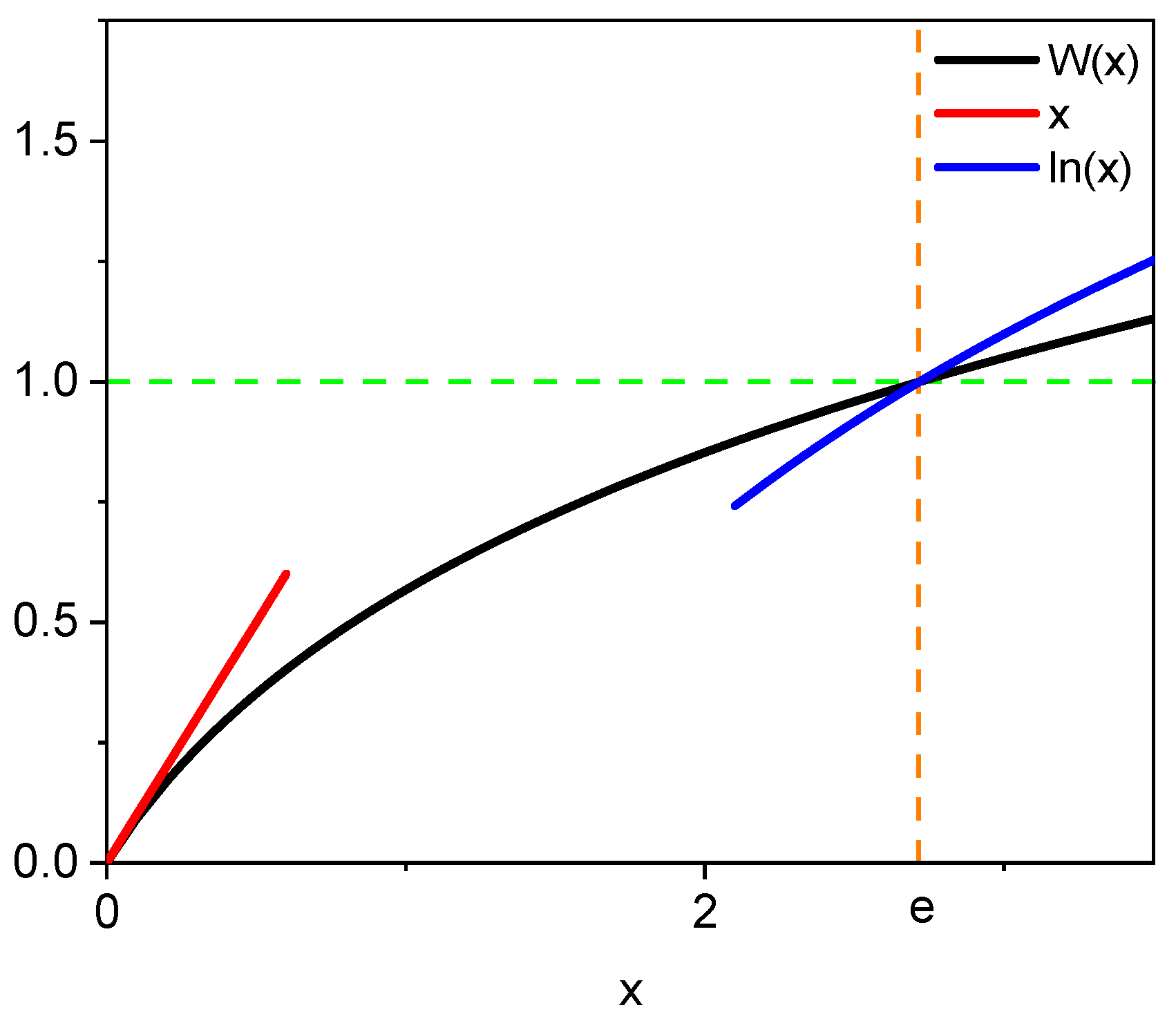
satisfies the LH equation with initial condition $C\left(0\right)=C_0$. $W\left(x\right)$ is the principal branch of the Lambert function. This is an analytical, monotone injective defined as the inverse of $f\left(x\right)=x{e}^x$ [21]. The plot of the Lambert function can be seen in Figure 4 (black line).

From now on, we will make an abuse of notation, and we will refer to the principal branch of the Lambert function as the Lambert function. Lambert function is quite frequently found in physical processes as Wien displacement’s law or the travelling time of a falling body in a medium with friction [21,22,23]. Also, the inverse of the Brillouin function, used in statistical mechanics to describe paramagnetism, is a particular example of a generalized Lambert function [21].

3.2. Approximations of the LH Solution

First, recall that $K_{e}C\left(t\right)=W\left(K_e{C}_0{e}^{K_e(C_0-k_{r}t)}\right)$ is a decreasing function of time (Equation (23)).

As the approximations of Equations (21) and (22) rely on the value of $K_{e}C$ versus 1, let us calculate the solution of the equation $K_{e}C\left(t\right)=1$. This value is the intersection of the green line of Figure 1 with the Lambert function graph. The result is as follows:

$$t_c={\displaystyle \frac{1}{k_{app}}}\left(K_e{C}_0+\ln \left(K_e{C}_0\right)-1\right)$$

(24)

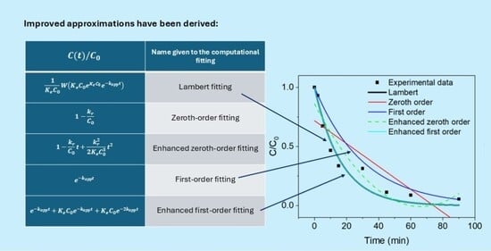
This parameter will be called critical time. By introducing the concept of critical time, we can study the kinetic process purely in a time scale: the linear first-order condition $K_{e}C\left(t\right)\ll 1$ is transformed into $t\gg t_c$ and the zeroth-order condition $K_{e}C\left(t\right)\gg 1$ into $t\ll t_c$.

It is important to highlight that t_c has time dimensions, but it is not a time in the physical sense, since it may have positive or negative values. A brief inspection of the expression used to define the critical time shows that

$$t_c>0 ⟺K_e>{\displaystyle \frac{1}{C_0}}.$$

(25)

The meaning of an extremely negative critical time, $t_c\ll 0$, requires an additional explanation. If $t_c\ll$0, then $t\gg t_c$, which is the condition for the photocatalytic process taking place under the first-order regime. That is, the entire experiment occurs in the first-order regime, with no existence of any time interval for which the zeroth order could apply.

Table 2. Mathematical formulation of the LH problem and its approximations, their respective solutions and the hypothesis assumed to arrive at these approximations.

Regime	Cauchy Problem (Differential Equation with Initial Condition)	$\mathbf{Analytic} \mathbf{Solution} \mathbf{of} \mathit{C}\left(\mathit{t}\right)$	${\mathit{K}}_{\mathit{e}}\mathit{C}\left(\mathit{t}\right)$ Hypothesis	${\mathit{t}}_{\mathit{c}}$ Hypothesis
Zeroth-order	$\left\{\begin{array}{c}{C}^{\prime }\left(t\right)=-k_r \\ C\left(0\right)=C_0\end{array}\right.$	$C_0-k_{r}t$	$K_{e}C\left(t\right)\gg 1$	$t\ll t_c$
First-order	$\left\{\begin{array}{c}{C}^{\prime }\left(t\right)=-k_r{K}_{e}C\left(t\right) \\ C\left(0\right)=C_0\end{array}\right.$	$C_0{e}^{-k_{app}t}$	$K_{e}C\left(t\right)\ll 1$	$t\gg t_c$
General solution	$\left\{\begin{array}{c}{C}^{\prime }\left(t\right)=-{\displaystyle \frac{k_r{K}_{e}C\left(t\right)}{1+K_{e}C\left(t\right)}} \\ C\left(0\right)=C_0\end{array}\right.$	${\displaystyle \frac{1}{K_e}}W\left(K_e{C}_0{e}^{K_e\left(C_0-k_{r}t\right)}\right)$

summaries the mathematical formulation of the LH problem and its approximations yielding zeroth-order and first-order regimes, their respective solutions and the assumptions made to arrive at them.

After all, the solution $C$ described by the $W$ function is the generalization of the first-order or zeroth-order regime depending on the value of $K_{e}C\left(t\right)$. The more we approach the assumptions validating a certain regime, the more the values of $k_{app}$ (for first order) and $k_r$ (for zeroth order) obtained from the general solution and the approximated solution should coincide, as they are the limit cases of it. A small relative error between these constants might be an indicator of how close we are to a particular regime, but the main test for ascribing an experiment to a regime should be the calculation of the critical time, as it is a direct translation of the value $K_{e}C\left(t\right)$. Similarly, other nonphysical results, such as obtaining negative $k_r$ and $K_e$ ratios in a particular regime, would be indicative for discarding it.

3.2.1. First-Order Regime

For the linear regime,

$$K_{e}C\left(t\right)\ll 1 \mathrm{for} \mathrm{all} t\ge 0; K_{e}C\left(0\right)=K_e{C}_0\ll 1.$$

In this case, the Lambert function (Equation (23)) and its argument can be replaced by their first-order Taylor series ($W\left(x\right)\approx x,x{e}^x\approx x)$ around $K_e{C}_0$ at a fixed time:

$$K_{e}C\left(t\right)=W\left(K_e{C}_0{e}^{K_e\left(C_0-k_{r}t\right)}\right)\approx K_e{C}_0{e}^{K_e\left(C_0-k_{r}t\right)}\approx K_e{C}_0{e}^{-k_{app}t},$$

(26)

which is the solution of the first-order regime, as seen comparing this equation with Equation (21).

If we want a more accurate expression for the first-order regime, we could keep the first order of $C\left(t\right)/C_0$ Taylor series for $K_e{C}_0$. This yields the following:

$${\displaystyle \frac{C\left(t\right)}{C_0}}\approx e^{-k_{app}t}+K_e{C}_0{e}^{-k_{app}t}+K_e{C}_0{e}^{-2k_{app}t}.$$

(27)

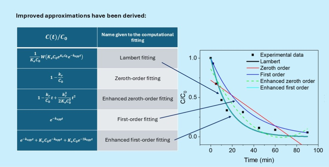
This fitting, which could be called the “enhanced first-order solution”, is much easier computationally than the adjustment of the general solution, and it permits the obtention of all ratios involved.

3.2.2. Zeroth-Order Regime

In the case of the zeroth-order regime,

$$K_{e}C\left(t\right)\gg 1 \mathrm{for} \mathrm{all} t\ge 0, \mathrm{and} K_e{C}_0\gg 1.$$

As $t\ll t_c,$ then the argument of the Lambert function

$$K_e{C}_0{e}^{K_e(C_0-k_{r}t)}\gg K_e{C}_0{e}^{K_e(C_0-k_r{t}_c)}=e.$$

(28)

The Lambert function W(x) is known to have an asymptotic series when $x>e$, whose first term is $W\left(x\right)\approx \mathrm{l}\mathrm{n}\left(x\right)$ [20], then

$$K_{e}C\left(t\right)=W\left(K_e{C}_0{e}^{K_e\left(C_0-k_{r}t\right)}\right)\approx \mathrm{l}\mathrm{n}\left(K_e{C}_0{e}^{K_e\left(C_0-k_{r}t\right)}\right)=K_e(C_0-k_{r}t)+\mathrm{l}\mathrm{n}\left(K_e{C}_0\right)$$

(29)

As $K_e{C}_0\gg \ln \left(K_e{C}_0\right)$ and $K_e{C}_0\gg 1$, then

$$K_{e}C\left(t\right)={K_e(C}_0-k_{r}t),$$

(30)

which corresponds to the zeroth-order solution of Equation (22).

As in the prior case, we could obtain a computationally powerful expression for this fitting. In the zeroth-order regime, whose solution is a linear tendency, small corrections could be enhanced by a quadratic term. As our solution is analytic, we could fit the data to the Taylor polynomial of second-order in t of the function. It is known that the Taylor series of the quotient is as follows:

$${\displaystyle \frac{C\left(t\right)}{C_0}}\approx 1-{\displaystyle \frac{k_{app}}{1+K_e{C}_0}}t+{\displaystyle \frac{k_{app}^2}{2{\left(1+K_e{C}_0\right)}^3}}{t}^2\approx 1-{\displaystyle \frac{k_r}{C_0}}t+{\displaystyle \frac{k_r^2}{{2K}_e{C}_0^3}}{t}^2.$$

(31)

Fitting the data to the quadratic polynomial $p\left(t\right)=c_0+c_{1}t+c_2{t}^2$, simple expressions for the parameters can be achieved:

$$k_r=-c_1{C}_0;K_e={\displaystyle \frac{c_1^2}{2c_2{C}_0}}$$

(32)

This method, which could be seen as the “enhanced zeroth-order solution”, is extremely powerful, as it can drop the two parameters with a simple parabolic fitting.

Table 3. Mathematical adjustments to LH equation and its several approximations.

$\mathit{C}\left(\mathit{t}\right)/{\mathit{C}}_0$ Form	Name Given to the Computational Fitting
${\displaystyle \frac{1}{K_e{C}_0}}W\left(K_e{C}_0{e}^{K_e{C}_0}{e}^{-k_{app}t}\right)$	Lambert fitting
$1-{\displaystyle \frac{k_r}{C_0}}t$	Zeroth-order fitting
$1-{\displaystyle \frac{k_r}{C_0}}t+{\displaystyle \frac{k_r^2}{{2K}_e{C}_0^3}}{t}^2$	Enhanced zeroth-order fitting
$e^{-k_{app}t}$	First-order fitting
$e^{-k_{app}t}+K_e{C}_0{e}^{-k_{app}t}+K_e{C}_0{e}^{-2k_{app}t}$	Enhanced first-order fitting

subsumes all the above approximations.

3.3. Numerical Treatment of the LH Solution

To link experimental data to the mathematical model, the Beer–Lambert law states that the concentration of pollutant, $C\left(t\right)$, has a linear relationship with light absorption, $A\left(t\right)$. Then, we can calculate the quotients of experimental absorption data and link them with the general closed solution:

$${\displaystyle \frac{A\left(t\right)}{A\left(0\right)}}={\displaystyle \frac{C\left(t\right)}{C\left(0\right)}}={\displaystyle \frac{1}{K_e{C}_0}}W\left(K_e{C}_0{e}^{K_e{C}_0}{e}^{-k_{app}t}\right)$$

(33)

This function describing the relative concentration (Equation (33)) has some mathematical subtleties which should be carefully considered. First, this quotient of concentrations can be adjusted to the following function, where $\alpha =K_e{C}_0$ and $\beta =k_{app}$:

$${\displaystyle \frac{C\left(t\right)}{C_0}}={\displaystyle \frac{1}{\alpha }}W\left(\alpha e^{\alpha }{e}^{-\beta t}\right).$$

(34)

This function may encounter some problems due to the magnitude orders of $\alpha$ and $\beta$. The case of $\beta$, which is an apparent rate, is usually between 10⁻³ and 10⁻² min⁻¹; $\alpha$ tends to be around 10⁻¹ L/mg, always depending on the characteristics of each experiment [24,25]. In particular, the main problem arises in the fitting of $\alpha$, which is a minute value on the denominator. Therefore, small variations in $\alpha$ can affect fitting. This non-linear fitting should be solved with iterative algorithms, such as Levenberg–Marquandt [26,27,28], in which the least squares problem would reduce the sum of residuals by approaching $\alpha$ and $\beta$ to zero. Hence, special attention must be paid to avoid saturating the numerical minimization with the imposed lower boundaries.

Before going further, some considerations about the error determination are needed. As mentioned, the fitting parameters must be nearly close to zero in both cases, and the only physical restriction that the parameters have is that they must be positive. This poses an intrinsically ill-conditioned problem. Consequently, the errors associated with the fitted parameters cannot be calculated accurately. It is possible to estimate the errors of a fit using the variance–covariance matrix, which depends on the Jacobian matrix of the function evaluated at the fitted parameters [26,27,28,29]. However, they would not provide practical information for a confidence interval, as the derivative of the function would enlarge it considerably.

General results might be derived to set conditions for these boundaries [27,29], or to explore the implementation of modified least square methods, such as Ridge regression [30]. However, such an elevated level of optimization is beyond the scope of this work. In our case, keeping in mind the above reasons during the mathematical treatment, we have set the lower boundaries at zero for both parameters, proving with several initial conditions until obtaining fitted parameters that did not saturate them.

Despite the complexity we have described, the solution we propose for the Lambert function has a major advantage that must be emphasized. Whereas the customary approximations of the LH equation can only find k_app (from the first-order solution) or k_r (from the zeroth-order solution), with this method, both ratios are determined successively in one experiment. This eliminates the need for an additional isotherm to calculate the value of K_e without [31], or for multiple experiments where only one parameter varies to build a linear regression [32,33]. Hence, it is compulsory to tackle a deeper study of the quotient $C/C_0$ in order to achieve simpler computational expressions, but without losing the main advantage of finding $k_r$ and $K_e$ simultaneously by solving the exact equation.

4. Validation of the Model with Experimental Results

At this point, it is not our aim to find the best experimental conditions and/or photocatalyst, but to validate the theorical model to consolidate it. The main virtue of this model is to rule out, mathematically, one regime or another, instead of assuming canonically that the experiment follows a particular regime, as is often recurrently seen in the literature. For that, the model has been tested with two sets of samples of commercial powder which have been commented on in the experimental method section: on the one hand, two experiments using different quantities of anatase as tester to degrade several MB dissolutions (experiments #1 and #2 of Table 1), and two other identical experiments having the same mass of catalyst and concentration of MB dissolution, but using ZnO as catalyst (experiments #3 and #4). The idea of using these quantities is to provide two distinguishable scenarios: one showing a clear first-order degradation (anatase experiments), and the other showing that the data are not so easy to assign to a specific tendency, and therefore, there is a more delicate discussion regarding how to exploit the power of the model (ZnO experiments).

Photocatalysis experiments using powder as catalysts have been performed. Whatever the samples, the effectiveness of the photocatalysis is calculated from the degradation efficiency at a time t, following Fernández-Calzado et al. [34]:

$$D\mathrm{\%}={\displaystyle \frac{C\left(t\right)-C_0}{C_0}}$$

(35)

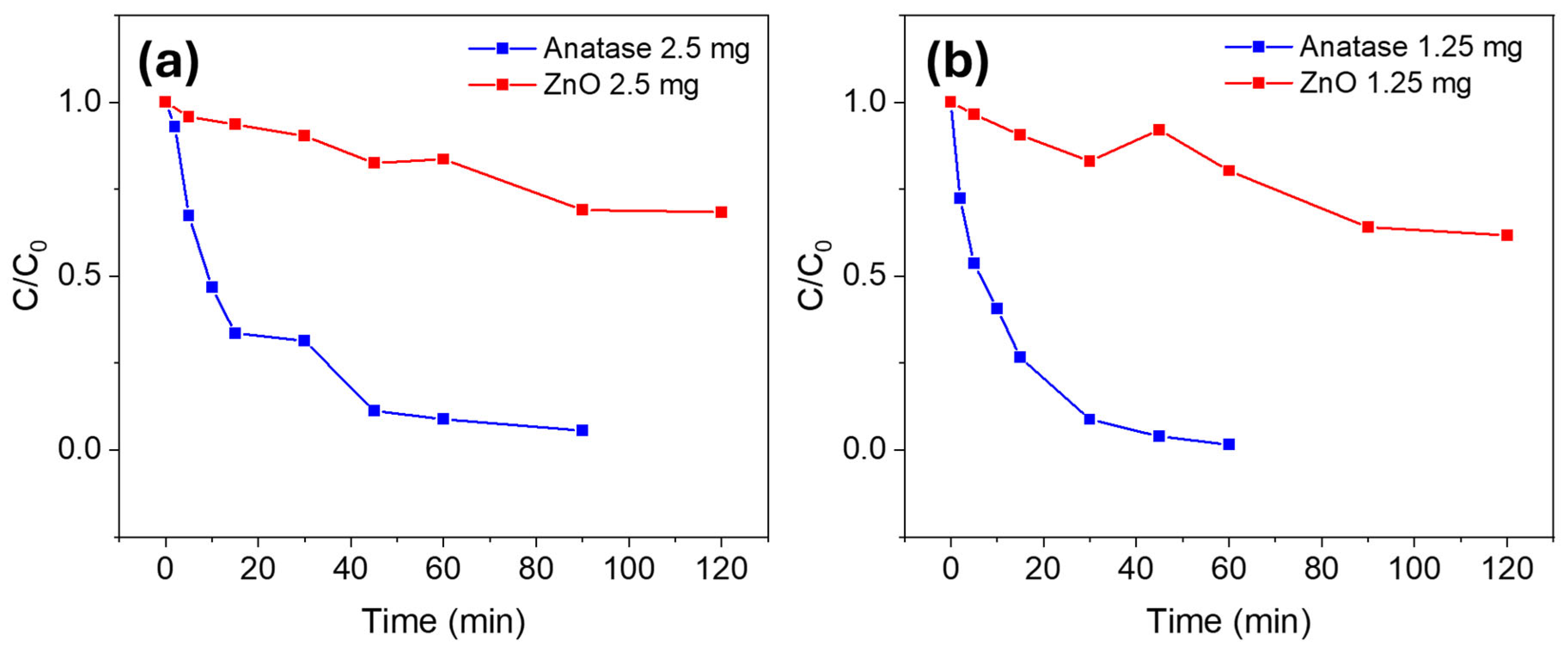
Figure 5 shows the evolution of the quotient $C\left(t\right)/C_0$. As seen, anatase degrades better than ZnO in all experiments having the same mass of catalyst and the same concentration of MB. Indeed, the experiments with anatase were ended before 120 min, since the dissolution had already been completely degraded. Using 2.5 mg of catalyst in a MB dissolution of 2.5 ppm in volume (Figure 5a), anatase reached ~95% in 90 min, while ZnO reached ~32% in two hours. For the case of 1.25 mg of catalyst in a MB dissolution of 1.25 mg in volume (Figure 5b), anatase nearly degraded completely (~99%), whereas the ZnO degradation efficiency, around ~40%, is considerably lower than of anatase. The control experiment, performed to monitor the degradation efficiency of the photolysis, has given an efficiency of ~13% and a degradation ratio is $\lambda =9.65·{10}^{-4}$ min⁻¹. From what we can conclude, the photolysis effect does not play the main role in the experiments. In addition, the tendency of degradation of anatase experiments is quite like an exponential decay, which would correspond to first-order degradation. Conversely, ZnO degradation does not have such a recognizable tendency to decay.

To deepen into the kinetic study, several fittings have been performed to all experiments. The fittings having been performed, a quantitative indicator of the goodness of fit is the determination coefficient, R², which is a canonical tool in regression analysis. A R² coefficient close to 1 evidences the fact that the model explains the data accurately. If $y_i$ represents the experimental data, $\widehat{y_i}$ the fitted data, and $\overline{y}$ the mean of the data, the determination coefficient is calculated as follows [29]:

$${\mathrm{R}}^2=1-{\displaystyle \frac{SSR\left(Squared sum of residuals\right)}{SST\left(Squared sum of totals\right)}}=1-{\displaystyle \frac{{\sum }_{i=1}^n{\left(y_i-\widehat{y_i}\right)}^2}{{\sum }_{i=1}^n{\left(y_i-\overline{y}\right)}^2}}.$$

(36)

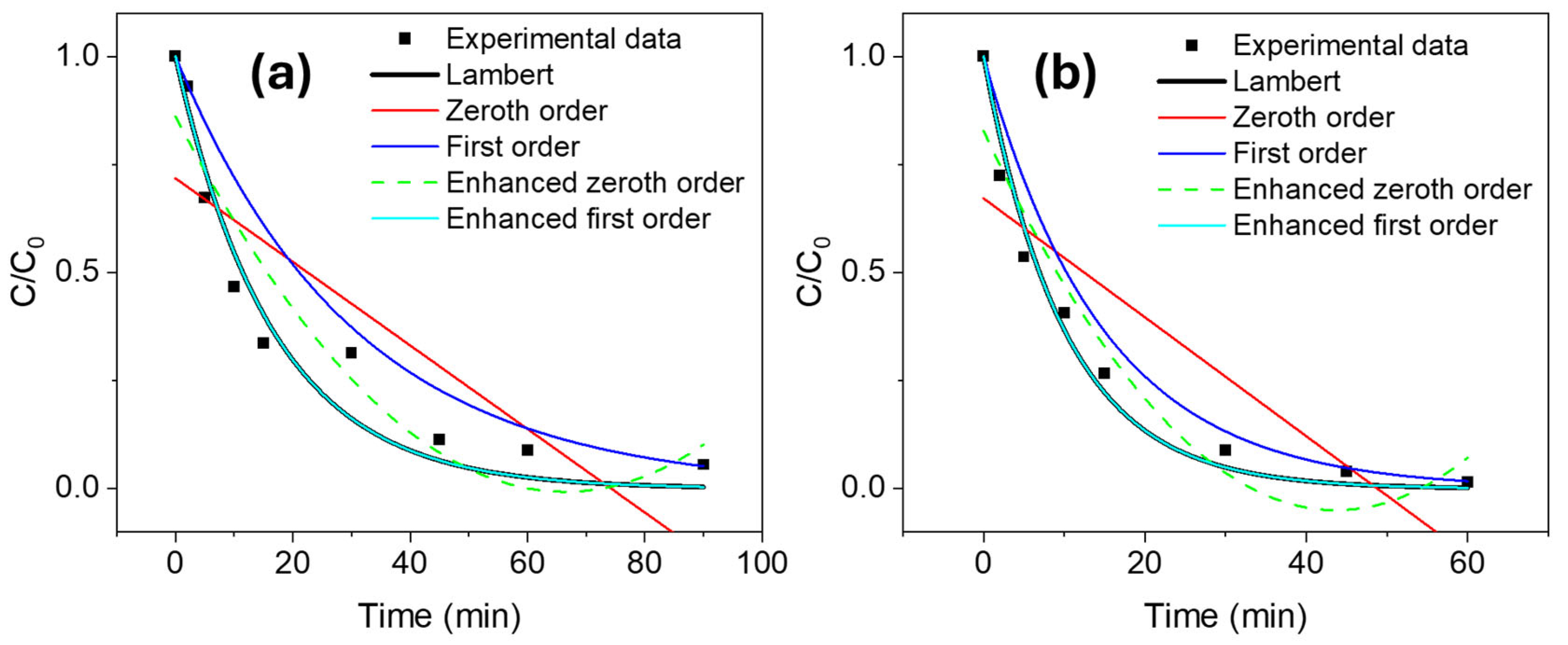
Anatase experiments will be studied first. Figure 6 shows the fitting of experiments #1 and #2 to the previously derived functions: Lambert fit, zeroth-order fit, first-order fit, enhanced zeroth-order fit and enhanced first-order fit.

Table 4. Parameters obtained by all fittings for anatase experiments #1 and #2.

		Anatase 2.5 mg (#1)	Anatase 1.25 mg (#2)
Lambert fit	Ke	1.4 × 10−9	2.0 × 10−11
	kr	4.2 × 107	5.1 × 109
	kapp	0.061	0.100
	tc	−338	−254
	R2	0.95	0.98
Zeroth-order fit	kr	0.024	0.017
	R2	0.70	0.73
First-order fit	kapp	0.033	0.067
	R2	0.81	0.91
Enhanced zeroth-order fit	Ke	−0.038	−0.029
	kr	0.065	0.050
	R2	0.89	0.93
Enhanced first-order fit	kapp	0.061	0.100
	Ke	0.001	0.002
	kr	61	50
	R2	0.95	0.98

shows the parameters obtained from these calculations. Figure 6a shows the kinetic study for experiment #1 (2.5 mg of anatase in MB solution having 2.5 ppm in volume), and Figure 6b shows that of experiment #2 (1.25 mg of anatase in MB solution having 1.25 ppm in volume). As seen, the first order does not describe the data completely, since R² = 0.81. While this value is not bad, is not as good as we would like. Instead, the Lambert fitting, which fits the data to the analytical real solution, describes the data accurately. This visual fact is supported by a R² = 0.95, which proves quantitatively the suitability of the model. Furthermore, the enhanced first-order fitting completely overlaps with this Lambert fit and has its same R². This means that, in this case, the first-order enhanced solutions, which is an exponential-like fit and mathematically simpler than the Lambert fit, describes the data just as well as the Lambert fit. This reasoning highlights the advantages of the derivation of these enhanced approximations: as well as describing the data better than the traditional first-order approach, it enables the two fit constants to be fitted at the same time. Indeed, enhanced first-order fitting is better than the Lambert fit because it yields values of $K_e$ and $k_r$ in consonance with the literature [24,25], whereas the Lambert parameters seem unrealistic. This is due to the fact that the pure Lambert fit is an ill-conditioned problem, which could give mathematically accurate and unphysical results. On the other hand, enhanced first-order fitting has a simpler expression, so its results are physically more reliable than the prior ones. Nevertheless, the Lambert fit is essential to derive these powerful approximations. Furthermore, the negative critical time also supports the fact of performing the experiment perpetually throughout the first-order regime. At the same time, the first order is assessed since the zeroth order can be completely discarded for several reasons: their R² coefficients are poorer than those of the first order; they do not describe well the evolution of the data; and negative K_e and k_r ratios are derived by the enhanced zeroth-order fitting, which has no physical meaning, and sometimes C/C₀ < 0, which also makes no physical sense.

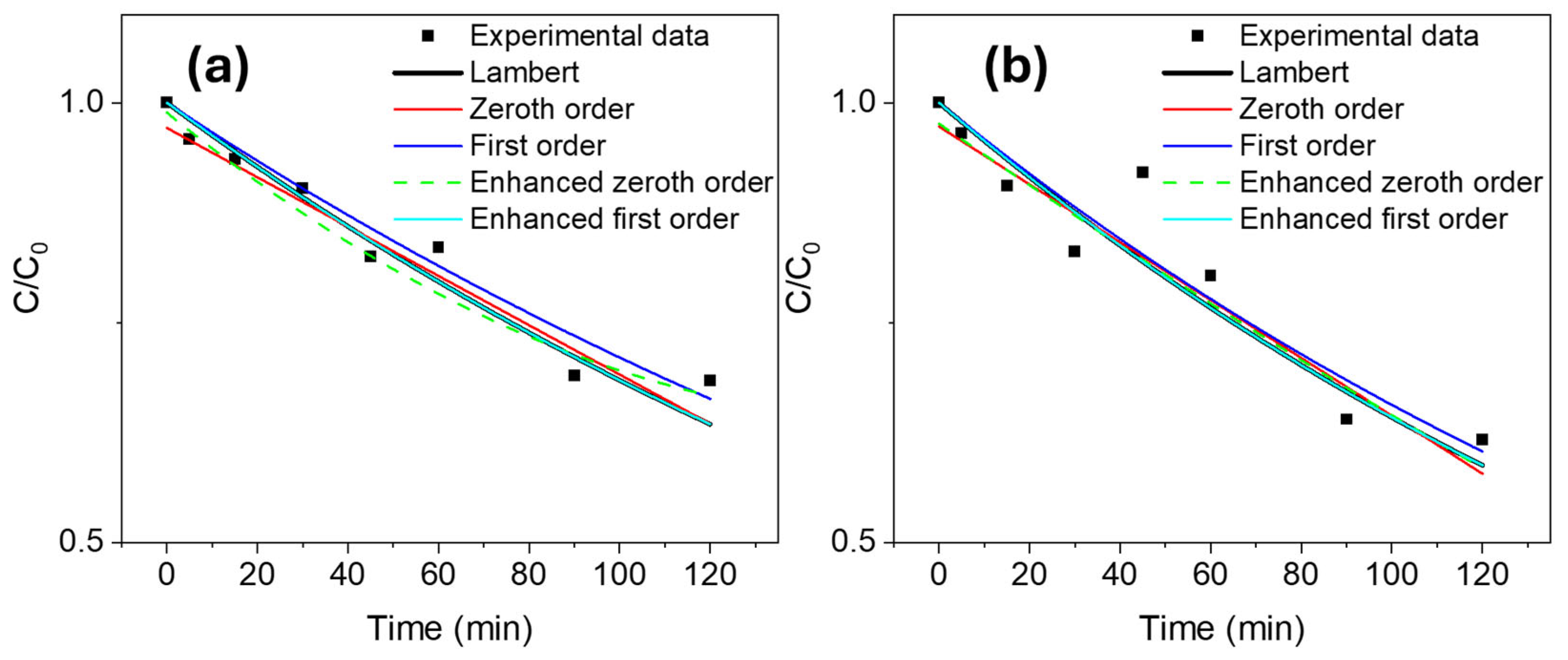
Now, let us turn to the ZnO kinetics. Figure 7a shows the results and fittings of experiment #3 (2.5 mg of ZnO in MB solution having 2.5 ppm in volume), and Figure 7b those of experiment #4 (1.25 mg of ZnO in MB solution having 1.25 ppm in volume). The results appear in

Table 5. Parameters obtained by all fittings for ZnO experiments #3 and #4.

		ZnO 2.5 mg	ZnO 1.25 mg
Lambert fit	Ke	1.8 × 10−7	2.3 × 10−5
	kr	4.1 × 104	189
	kapp	0.012	0.004
	tc	−4.30 × 103	−2.59 × 103
	R2	0.94	0.88
Zeroth-order fit	kr	0.007	0.041
	R2	0.94	0.89
First-order fit	kapp	0.003	0.004
	R2	0.92	0.89
Enhanced zeroth-order fit	Ke	−0.015	−0.002
	kr	0.010	0.004
	R2	0.96	0.89
Enhanced first-order fit	kapp	0.004	0.004
	Ke	0.001	0.002
	kr	3.85	2.24
	R2	0.94	0.88

. Unlike anatase experiments, the tendency of the data is not so clear, as all the fittings overlap. For this reason, it is necessary to make a detailed discussion instead of assuming first-order degradation carelessly, especially when all R² values are quite close to each other. Firstly, the inspection of the kinetic ratios obtained for the zeroth order reveals that they are negative, which rules out this degradation regime. In addition, the negative critical time also hints at first-order degradation. For these reasons, the first-order degradation is established by discarding the zeroth-order regime. As in the prior case, the constants obtained by the enhanced fitting have more physical meaning than those obtained by the Lambert function. Finally, we might conclude that this first-order degradation is weaker than that observed in anatase experiments (Figure 6), since the overlap of all fittings attenuates the evidence for a clear first-order degradation. Further analyses are required to fully elucidate this behaviour; however, it seems plausible that it is related to the reduced adsorption sites.

5. Conclusions

The analytical solution of the Langmuir–Hinshelwood kinetics has been found in terms of the typical degradation ratios k_r, K_e and k_app. Although it can encounter some problems in performing the mathematical fitting due to the computational treatment, it can provide the two ratios involved in the LH process successively. To overcome this obstacle, several enhanced approximations of the analytic solution for first-order and zeroth-order LH kinetics have also been derived, which permit calculating more ratios than typical approximations have been obtained. A parameter called critical time, only dependent on the experiments and able to discriminate between the first order and zeroth order, has been settled. Finally, the model has been tested with selected MB solutions using ZnO and anatase as catalysts. A first-order regime is observed in all cases, supported by a negative critical time in all experiments. In the case of anatase, the customary first order describes well the experimental data, but the enhanced first-order approximation and Lambert function fit them perfectly. In the case of ZnO, a first-order regime can be settled by ruling out the possibility of having a zeroth-order regime due to the obtention of negative LH ratios.

Although our model is quite robust, further experimental studies should be performed to further validate it. In particular, we have chosen two photocatalysts well known for their good performance, but it would be very interesting to check the results with other materials in which the presence of the different regimes may be particularly relevant.