Article

Identifying Winter Light Stress in Conifers Using Proximal Hyperspectral Imaging and Machine Learning

by
Pavel A. Dmitriev
1,*,
Boris L. Kozlovsky
1,
Anastasiya A. Dmitrieva
1,
Mikhail M. Sereda
2,
Tatyana V. Varduni
1 and
Vladimir S. Lysenko
1
1
Botanical Garden, Academy of Biology and Medicine, Southern Federal University, Rostov-on-Don 344006, Russia
2
Department of Botany and Bioresources, Don State Technical University, Rostov-on-Don 344000, Russia
*
Author to whom correspondence should be addressed.
Stresses 2025, 5(4), 62; https://doi.org/10.3390/stresses5040062
Submission received: 12 September 2025 / Revised: 14 October 2025 / Accepted: 20 October 2025 / Published: 21 October 2025
(This article belongs to the Section Plant and Photoautotrophic Stresses)

Abstract

The development of remote methods for identifying plant light stress (LS) is an urgent task in agriculture and forestry. Evergreen conifers, which experience winter light stress (WLS) annually, are ideal subjects for studying the mechanisms of light stress and developing identification methods. Proximal hyperspectral imaging (HSI) was used to identify WLS in Platycladus orientalis. Using the random forest (RF), the spectral characteristics of P. orientalis shoots were analysed and the conditions ‘Winter Light Stress’ and ‘Optimal Condition’ were classified with high accuracy. The out-of-bag (OOB) estimate of the error rate was only 0.35%. Classification of the conditions ‘Cold Stress’ and ‘Optimal Condition’—with an OOB estimate of error rate of 3.19%—can also be considered successful. The conditions ‘Winter Light Stress’ and ‘Cold Stress’ were more poorly separated (OOB error rate 15.94%). Verifying the RF classification model for the three states ‘Optimal condition’, ‘Cold stress’ and ‘Winter Light Stress’ simultaneously using data from the crown field survey showed that the ‘Winter Light Stress’ state was well identified. In this case, ‘Optimal condition’ was mistakenly defined as ‘Cold stress’. The following vegetation indices were significant for identifying WLS: CARI, CCI, CCRI, CRI550, CTRI, LSI, PRI, PRIm1, modPRI and TVI. Therefore, spectral phenotyping using HSI is a promising method for identifying WLS in conifers.

Graphical Abstract

1. Introduction

Accurate, rapid and technologically feasible non-invasive methods for identifying plant stress across a wide spatial range (from cells to land areas) are urgently needed in agriculture and forestry [1,2,3]. Stresses of an abiotic or biotic nature can have a significant negative impact on plant growth and productivity, potentially leading to death [4,5].
There is a wide range of abiotic stress factors related to the growth and development of plants, such as temperature, drought, heat, cold and many more [6,7]. Among abiotic stresses, winter light stress (WLS) in evergreen conifers growing in temperate and boreal climates deserves special mention. Coniferous plants here are exposed to prolonged periods of sub-zero temperatures and intense light every winter [8]. This combined effect causes chronic light stress (LS) in conifers, which is why they can be considered the most adapted to this phenomenon among other plants [9]. Against the backdrop of the cessation of growth processes, exposure to low positive and negative temperatures causes a decrease in the photosynthetic activity of plants [9,10,11]. This decrease is due to the limitation of the speed of photosynthetic electron transport and the Calvin cycle [11,12]. At the same time, chlorophyll, whose content in coniferous leaves does not decrease significantly during acclimatisation [13], captures light energy throughout the winter. Under such conditions, most of the absorbed light energy cannot be used for photosynthesis [10,14]. Excessive light energy causes photoinhibition and leads to the formation of reactive oxygen species (ROS), which can cause significant photooxidative damage [15].
During evolution, plants have developed a complex set of mechanisms to counteract LS [16,17].
Firstly, there is a limitation on the absorption of light energy. Chloroplasts can move to the anticlinal cell wall to achieve this [18]. The synthesis of coloured phenolic compounds (anthocyanins and carotenoids), which act as optical filters and light reflectors, increases [19]. Meanwhile, there is a moderate decrease in chlorophyll content [20].
Secondly, photoprotection is achieved through photochemical and non-photochemical quenching [21]. Photochemical quenching involves the scattering of excess chlorophyll excitation in the form of fluorescence, while non-photochemical quenching (NPQ) involves improving xanthophyll cycle pools and de-epoxidation of xanthophyll cycle components. NPQ is the fastest response of photosynthetic membranes to excess light [22]. Higher plants have two types of NPQ, which relax at different rates after exposure to excess light. These are fast-relaxing energy quenching (qE), which dominates in warm conditions, and slow-relaxing or persistent NPQ (qI), which dominates in winter and is characteristic of evergreen conifers [9,11,23].
Flexible thermal dissipation is based on the interconversion of xanthophyll pigments (violaxanthin—antheraxanthin—zeaxanthin, VAZ) to dissipate excess light energy in the form of heat, preventing potential damage to the photosynthetic apparatus. Flexible thermal dissipation is regulated on a daily basis. Sustained thermal energy dissipation is caused by changes in the xanthophyll pigment pool and is regulated seasonally [23,24]. During the process of stable quenching, zeaxanthin is not converted back to violaxanthin immediately after exposure to light ceases; its restoration requires several days of heating the needles [25]. Therefore, a consistently high level of zeaxanthin is a characteristic feature of conifers in winter. Unlike flexible thermal dissipation, stable quenching allows conifers to dissipate excess energy over a long period of time (including at night), thereby increasing their resistance to stress during winter [26].
Thirdly, ROS are neutralised by enzymatic and non-enzymatic mechanisms. During photorespiration, NADH is consumed, which protects the electron transport chain of photosynthesis [27].
Fourthly, it is a mechanism for repairing damaged photosystem II (PSII)—PSII repair occurs through the degradation and removal of D1 proteins from damaged PSII and the synthesis of D1 protein precursors [28].
Thus, WLS in conifers is a unique phenomenon, as it is generated simultaneously by two independent factors: excessive light and sub-zero temperatures. It is characterised by reduced photosynthetic capacity, consistently low maximum quantum efficiency of PSII (Fv/Fm) and consistently high zeaxanthin concentration, a combination of qE with qI, which dominates [8]. Evergreen conifers, for which WLS is an annually recurring seasonal phenomenon, can be considered convenient objects for studying the mechanisms of LS and developing methods for its identification.
Of the many methods of identifying stress in plants [2], spectral phenotyping is of particular interest for remote sensing [16,29,30], especially using hyperspectral imaging (HSI) [31,32]. Hyperspectral imaging allows spectral information to be obtained with very high spatial resolution and across a fairly wide spectral range (from 350 to 2500 nm). In addition, HSI offers several other advantages, including rapid information retrieval (with the option of real-time mode), extensive spatial coverage ranging from proximal to remote sensing, a non-invasive process and a high degree of automation [33,34]. The emergence of HSI has given impetus to the growth in the number of narrowband vegetation indices (VIs) [35,36]. Most VIs are structural indices and describe plant characteristics indirectly through the content of photosynthetic pigments and the leaf area index [37,38].
Based on the biochemical tendencies of adaptation of conifers to WLS, the total content of carotenoids (Ccar) can be observed as a predictor of stress during its spectral phenotyping. In addition to the Ccar, the ratio of the total chlorophyll content (Cchl) to the Ccar (Cchl/Ccar) is used to assess stress resistance [39]. Currently, there are several narrow-band VIs for assessing carotenoid content in plant leaves and crowns, as well as several VIs for assessing Cchl/Ccar. Zhou et al. [40] developed a combined carotenoid/chlorophyll ratio index (CCRI) in the form of the carotenoid index (CARI) divided by the red-edge chlorophyll index (CIred-edge). He et al. [41] also proposed a similar combined CCRI. The ratio of the carotenoid triangle ratio index (CTRI) with the CIred-edge was found least influenced by the Cchl–Ccar correlation and demonstrated ability for estimating Cchl/Ccar variability [42].
Recently, a modified photochemical reflectance index (modPRI515/550) has been proposed as a diagnostic tool to assess the interaction of LS with other abiotic stresses [43]. Several specialized VIs (LSI, LSIRed and LSINorm) for LS identification, developed on Ficus elastica, are also proposed [32]. Vegetation indices used to assess Ccar, Cchl/Ccar and LS are presented in Table 1.
Among the VIs presented in Table 1, CCI and PRI have proven to be very effective in describing the annual growth cycle of conifers [64,65,66]. The photochemical reflection index (PRI) effectively identifies LS in conifers [57]. It records daily and seasonal transformations of xanthophyll cycle pigments, which are associated with the plant’s response to excess light energy [67].
Machine learning (ML) methods are widely used for hyperspectral data analysis, with Random Forest (RF) leading the way in terms of frequency of use and prediction accuracy [68]. Deep machine learning (DML) methods show great promise in spectral phenotyping of plants [69], but have not yet surpassed ML methods in terms of performance and accuracy [70,71].
This study builds on previous results on the identification of dormancy and vegetation states in conifers, as well as spectral phenology of conifers based on HSI data [64,72]. Based on the analysis of these data and the brief overview of the literature presented in this study, the following hypothesis was put forward: ‘Accurate qualitative assessment of LS in evergreen conifers is possible using Ccar and Cchl/Ccar-sensitive VIs by constructing multivariate models based on ML algorithms’. To test this hypothesis, the following dataset was collected:
  • Time series of proximal HSI data of the sunlit side of conifers shoots at intervals of 7–10 days for the period from 14 February 2023 to 28 April 2025.
  • Time series of proximal HSI data of the shaded side of conifers shoots at intervals of 7–10 days for the period from 21 November 2024 to 28 April 2025.
  • Time series of photosynthetic pigment content in sunlit shoots for the period from 14 February 2023 to 28 April 2025.
  • Time series of maximum quantum yield of PSII (Fv/Fm) of photosynthesis of sunlit and shaded sides of shoots for the period from 31 July 2024 to 28 April 2025.

2. Results

2.1. The Nature of the Annual Cycle of Carotenoids and the Ratio of Chlorophylls to Carotenoids of P. orientalis Shoots

The annual CCar dynamics in P. orientalis has a clearly defined seasonal character. In autumn, against the background of low positive temperatures, CCar begins to grow sharply in shoots well illuminated by the sun, then stabilizes and in March, with the onset of spring and an increase in temperature, it begins to fall (Figure 1a). The difference in CCar content between summer and winter shoots is very large and averages about 70%. The annual dynamics of Cchl/Ccar has a similar character (Figure 1b). The dynamics of CCar and Cchl/Ccar are well matched with the dynamics of the average daily temperature (Figure 2).
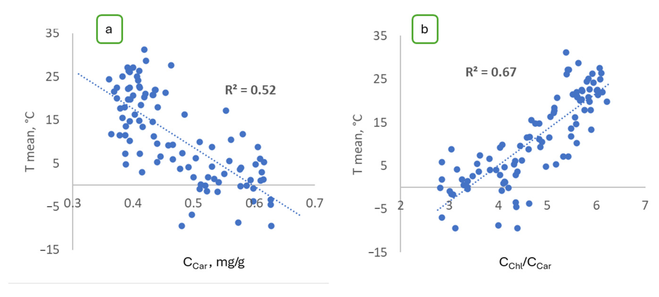
The CCar and Cchl/Ccar regressions from the average daily temperature have high coefficients of determination (0.52 and 0.67). The Cchl/Ccar ratio demonstrates a closer relationship with temperature.
It should be borne in mind that a sharp increase in the CCar content in the shoots of P. orientalis illuminated by the sun is correctly attributed not to the effect of temperature, but to the combined effect of negative temperature and high intensity light (WLS). Thus, both indicators (CCar and Cchl/Ccar) can be used with high reliability as predictors for assessing the WLS of conifers.

2.2. Estimation of the Maximum Quantum Yield of PSII Shoots of P. orientalis

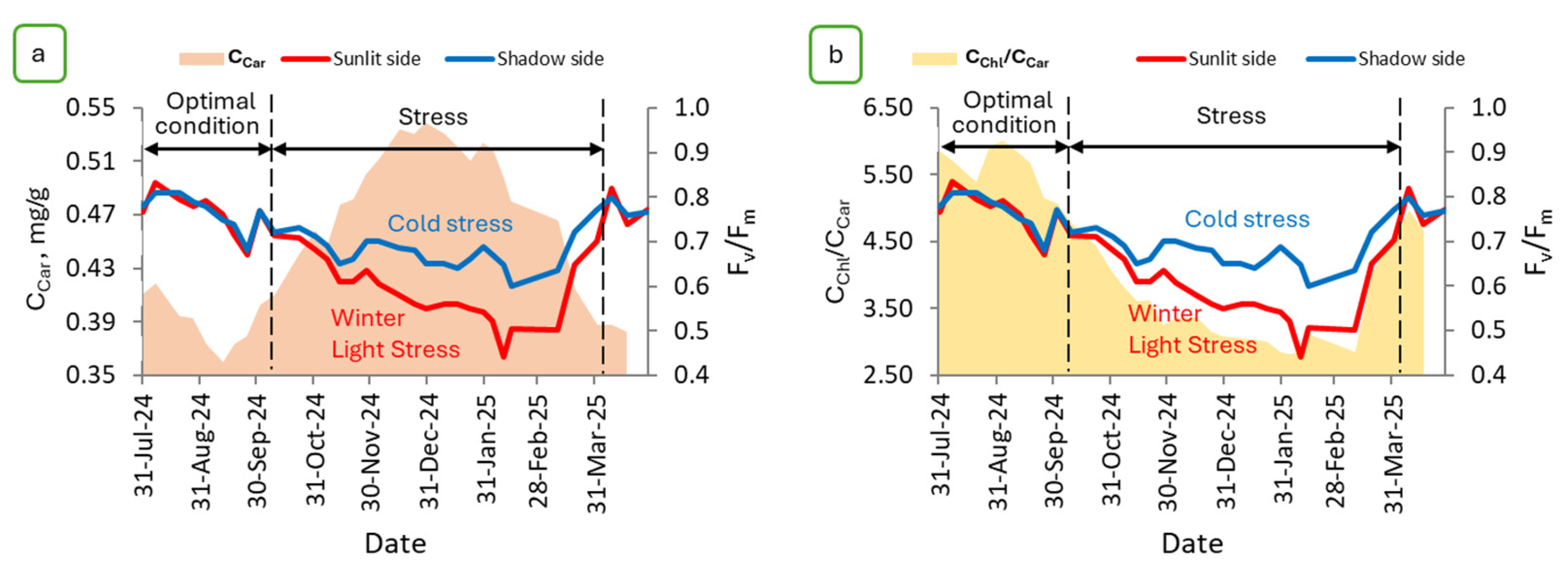
The Fv/Fm values of the illuminated and shaded sides of P. orientalis shoots during the active growing season (June, August 2024, April 2025) do not differ and approach the optimal value for conifers—750–800 mmol photons m−2s−1 (Figure 3). In September, the Fv/Fm values of the illuminated and shaded sides of the shoot begin to decrease and diverge. During the dormancy (from October to February), the shaded side shows a decrease in the Fv/Fm values from 800 to 670 mmol photons m−2s−1 (Figure 3a), the sunlit side shows a stronger decrease in the Fv/Fm values up to 450 mmol photons m−2s−1 (Figure 3b). At the same time, the greatest effect is observed in January and February, which are colder months in the region compared to November and December, while the duration of sunshine in these months is longer. Starting from the end of February and the beginning of March, the Fv/Fm values begins to grow sharply and by the end of March reaches the optimal value, the Fv/Fm value of the sunlit side and the shadow side of P. orientalis shoots align. Thus, in winter, PSII is inhibited in the conifers of P. orientalis shoots, which is a sign of the plant’s stress state. If we consider light and temperature as the main factors of PSII inhibition in coniferous plants in winter, then the shadow side of the shoot is P. orientalis is experiencing cold stress, the illuminated side of the escape is WLS (the result of the combined action of negative temperature and sunlight).
It was found that the Fv/Fm of the illuminated side correlates with CCar and Cchl/Ccar with high strength. Regressions of these characteristics have high coefficients of determination (Figure 4).
This confirms that CCar and Cchl/Ccar can be predictors of LS in conifers, so the use of carotenoid-sensitive VIs in WLS identification models may be effective.

2.3. The Results of the Exploratory Data Analysis for Vegetation Indices

An analysis of the distribution of VIs values using the Shapiro–Wilk tests and the chi-square criterion showed that the type of distribution does not correspond to the normal one. Therefore, the median was used as the average value for VIs, rather than the arithmetic mean.
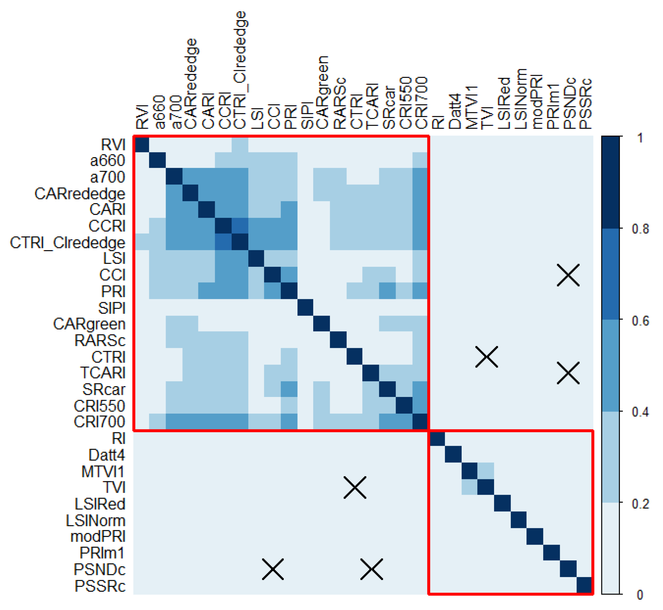
A matrix of pairwise coefficients of determination for the values of VIs was calculated (Figure 5). Strong coupling strength was noted for CCRI and CTRI/CIred-edge (CTRI/CIred-edge was excluded when building ML models), and average coupling strength was noted for the PRI, CCI, CARred-edge, CARI, and CRI700 groups. RI, Datt4, LSIRed, LSINorm, modPRI515/550, PRIm1, PSNDc and PSSRc have weak connections with all VIs.
The multicollinearity of the remaining 27 VIs was tested using the VIF. The results are presented in Table 2.
It has been established that this set of VIs is characterised by low multicollinearity. For all VIs, the VIF is below the critical level (VIF < 5). For 17 VIs, the VIF value is below 2.
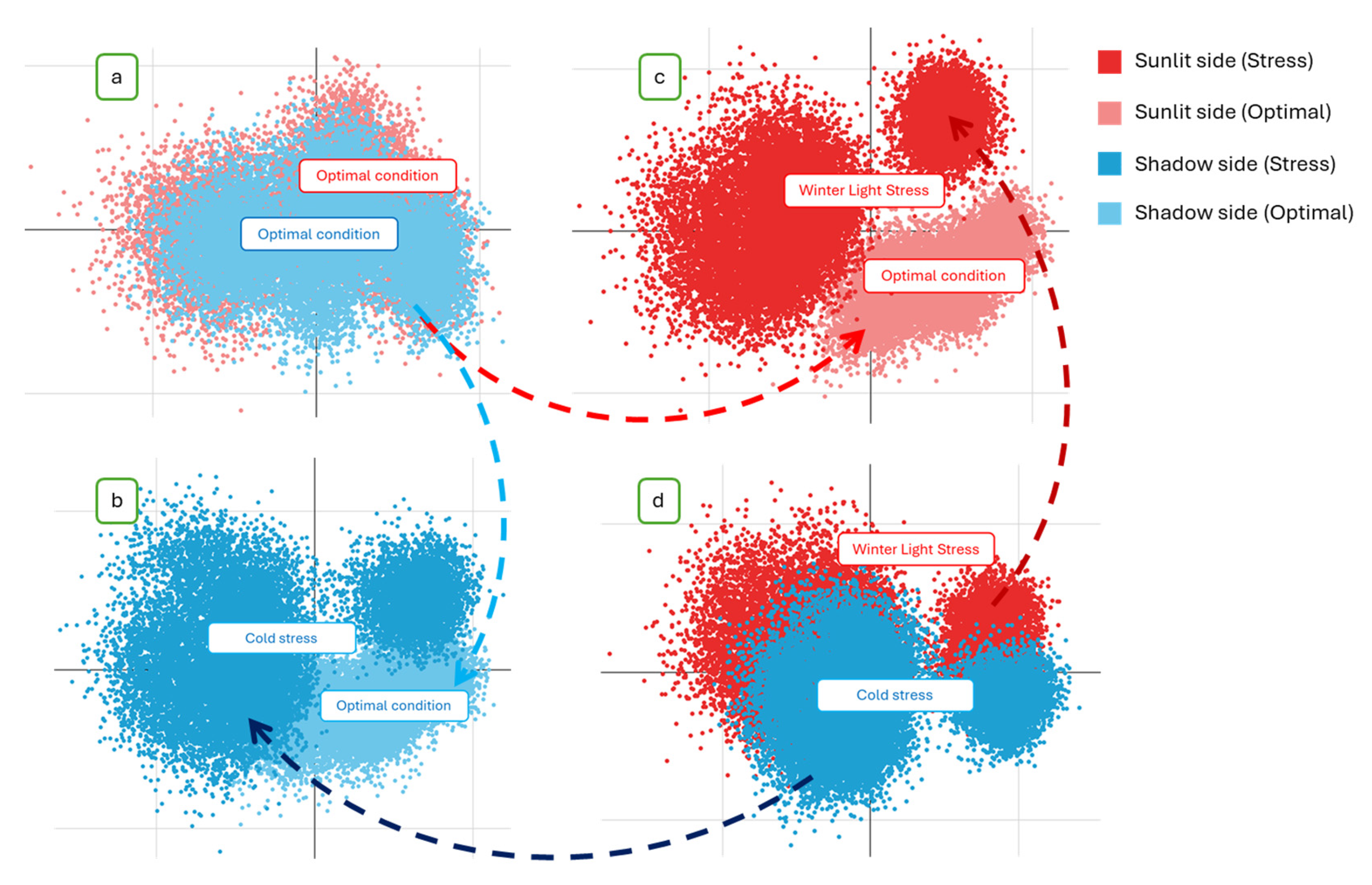
Using PCA, a preliminary comparative assessment of spectral states (expressed in terms of VIs values), sunlit and shaded sides of P. orientalis shoots in a state of winter dormancy and active vegetation was carried out (Figure 6).
Analysis of the data using PCA showed that at the beginning of meteorological vegetation period (MVP), the shoots of conifers do not experience LS—the spectral state of the illuminated and shaded sides of the shoots do not differ (Figure 6a). This state of the shoot can be determined as optimal. Spectral states of the sunlit side of the shoot during winter dormancy and active vegetation (optimal state) they are clearly distinguishable (Figure 6b), which can be attributed to the presence of WLS. The differences in the spectral states of the sunlit side of the shoot and its shadow side in winter (Figure 6d) indicate the possibility of classifying WLS and “pure” cold stress by spectral characteristics. Hereafter, “cold stress” refers to a condition that occurs under the influence of low positive and negative temperatures in the absence of high-intensity light. At the same time, the difference in the spectral states of the shade side of the shoot in the state of winter dormancy and active vegetation (Figure 6c) indicates the possibility of classifying cold stress and optimal plant condition.
The results of the PCA indicate the prospects of using VIs as independent variables in ML models (Table 1) to classify WLS, cold stress, and the optimal state of P. orientalis shoots.

2.4. Results of Modeling the Light Stress of P. orientalis Shoots

RF classification models of the following states of P. orientalis shoots were constructed: “Optimal condition”, “Cold stress” and “Winter Light Stress”. The model was trained in accordance with the allocation of P. orientalis states by Fv/Fm values and Ccar (Figure 1 and Figure 3). Confusion matrix pixel-based RF classification states of P. orientalis shoots in various combinations is presented in Table 2. Using the RF algorithm, it was possible to classify the conditions “Winter Light Stress” and “Optimal condition” with high accuracy. The out-of-bag (OOB) estimate of error rate was only 0.35%. The classification of conditions “Cold stress” and “Optimal condition”—OOB estimate of error rate—3.19%—should also be considered successful. The conditions of “Winter Light Stress” and “Cold stress” are worse (OOB estimate of error rate—15.94%). This is understandable, because WLS is the result of the combined action of high-intensity light and negative temperature, which induces cold stress. Therefore, the spectral states of shoots under cold stress and WLS may partially overlap (Figure 6d). When all three states (“Winter Light Stress”, “Cold stress” and “Optimal condition”) are simultaneously classified, only the “Optimal condition” state is classified with high accuracy (Table 3).
CCRI, CCI, CARI, PRI, and PRIm1 are of the greatest importance for the classification of “Winter Light Stress” and “Optimal condition” states (the first five VIs were selected in accordance with the contribution to the Mean Decrease Accuracy and Mean Decrease Gini values) (Figure 7a). The classification of conditions “Cold stress” and “Optimal condition”—CCRI, CARI, TVI, CRI550 and CTRI (Figure 7b). “Winter Light Stress” and “Cold stress”—CCI, PRI, CCRI, LSI and CARI (Figure 7c). ‘Winter Light Stress’, ‘Cold stress’ and ‘Optimal condition’—CCRI, CCI, PRI, CARI and PRIm1 (Figure 7d).
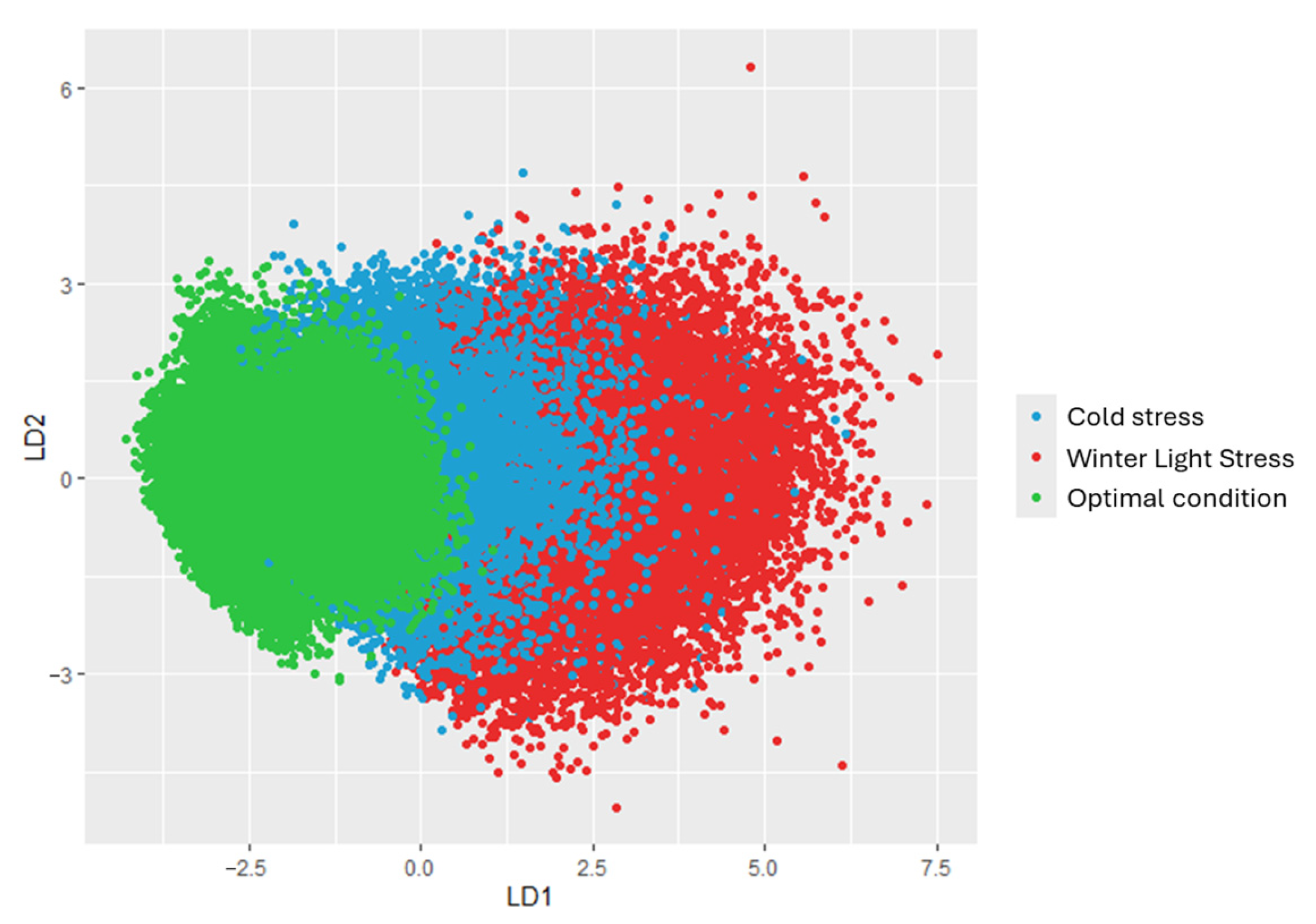
In parallel with the RF classification, the states of P. orientalis shoots were discriminated using the LDA. The results of step-by-step classification using a 10-fold cross-validated assessment of the correctness of the LDA, provided that the addition of the following factor does not increase accuracy by more than 1%, are presented in Table 4. The results of discrimination of P. orientalis shoot states using LDA are in good agreement with the results of RF classification in both accuracy and according to VIs, which were significant for the separation of states.
Figure 8 shows good discrimination of the “Winter Light Stress” and “Optimal condition” states and the overlap of these states with “Cold stress”.
RF model (‘Winter Light Stress’ & ‘Optimal condition’) was tested on a time series of hyperspectral images of the illuminated side of the shoots (Figure 9). It gave a good coincidence of the timing of WLS with the maximum Ccar and the minimum of negative temperatures.

2.5. Results of Testing the RF Model on Platycladus orientalis Crowns

To test the classification models of P. orientalis states on the crowns of a plant, it is necessary to pre-mark the crown pixels. At the moment, we do not have a technique with which it would be possible to objectively mark the ROI in a hyperspectral image according to the states ‘optimal state’, ‘cold stress’ and ‘winter light stress’. It is possible to generally characterize the condition of the plant based on the Fv/Fm and Ccar obtained from a sample of shoots from the crown, against the background of the daily temperature regime. Thus, the P. orientalis instances in the time series were marked up by state based on these indicators, and the accuracy of the model’s prediction was determined as the proportion of crown pixels assigned to this state.
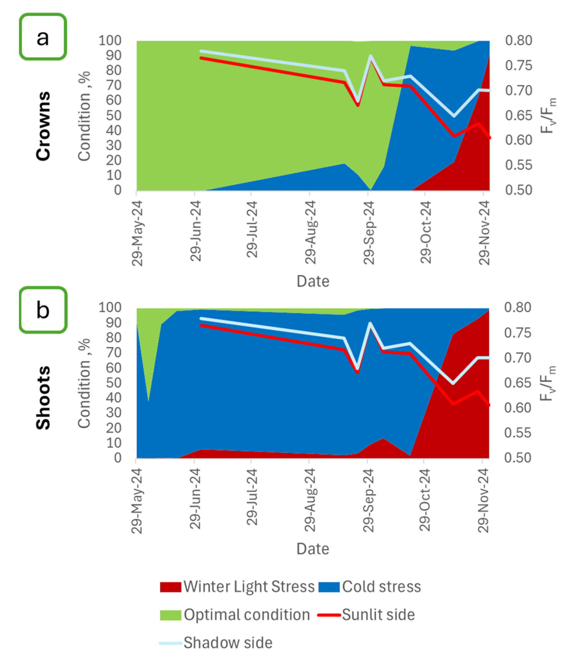
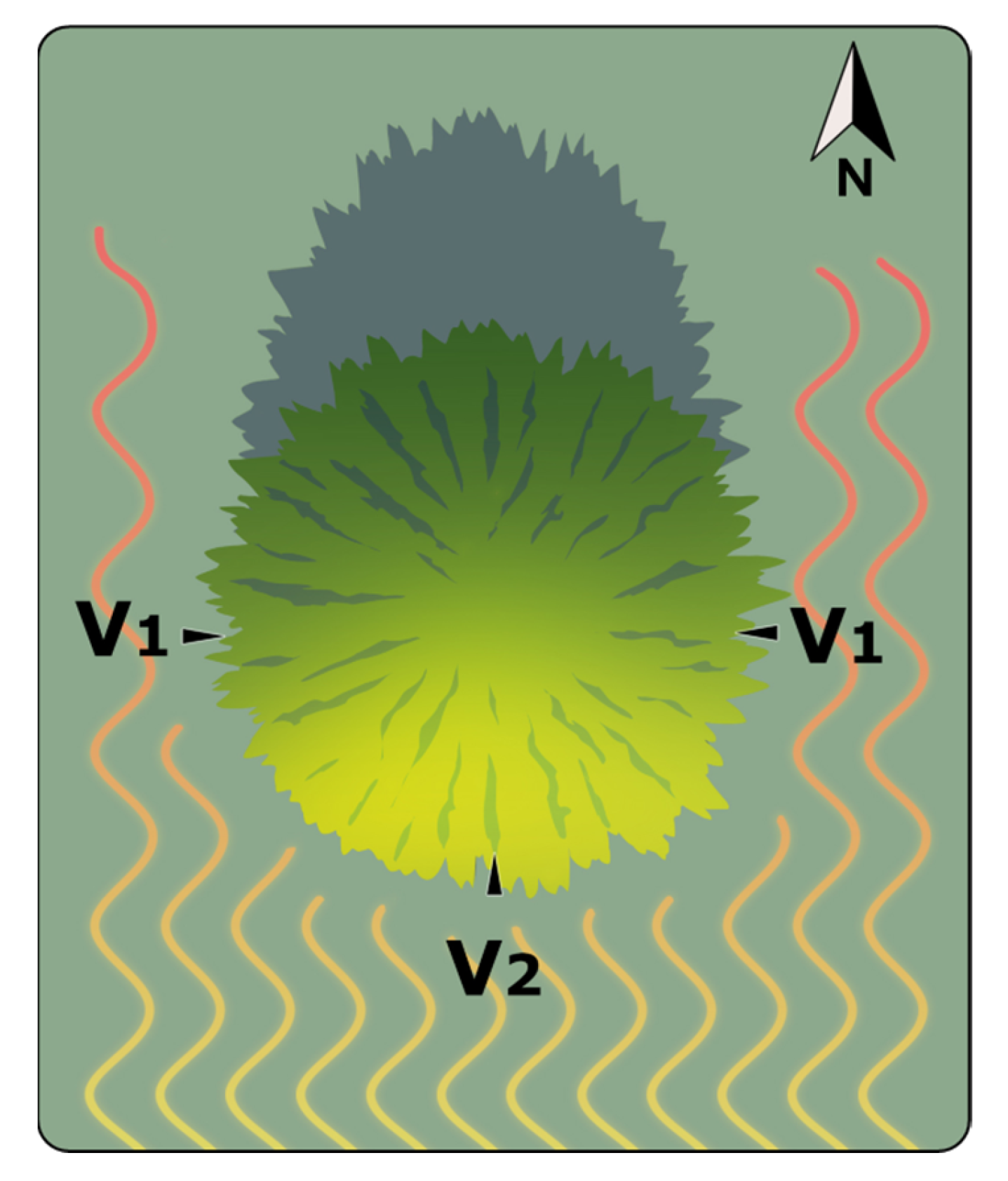
Testing of the RF model trained on P. orientalis shoots on its crowns showed that the condition ‘winter light stress’ is classified well (Figure 10a). However, the optimal condition on the crowns is not determined—the model ‘classifies’ it as ‘cold stress’. In order to make sure that no methodological errors were made during the experiment with the crowns, the model was tested on the shoots of these samples. Shoots were taken from the crowns in zone V2 (Figure 11) immediately after the field proximal HSI of the crowns, HSI was performed in the laboratory. Testing the model on shoots showed a good result for all three states (Figure 10b).
Thus, the RF model trained on the data of laboratory proximal HSI of shoots on crowns classifies the state of ‘winter light stress’ well and does not classify ‘cold stress’ and ‘optimal condition’. Further research is needed to solve this problem.

3. Discussion

Currently, there are about 600 species of conifers (Pinophyta) on the planet, many of which are dominant in boreal and temperate forests [73]. Boreal and temperate forests cover about 25% of the land area, mainly in the northern hemisphere in Eurasia and North America. The Boreal Forest is the largest natural forest in the world, covering about 25 million km2 [74]. Most temperate forests and many boreal forests are strongly affected by human resource use and management [75,76].
In general, the burden on boreal forests from abiotic and biotic factors is increasing [77]. The effects of climate change are expected to be particularly severe in temperate and boreal forests. Boreal forests adapted to critical negative temperatures may be particularly vulnerable to climate warming [78]. Given the important ecological function of coniferous forests, including their key role in global carbon and water cycles [79], monitoring of their condition is necessary.
Winter light stress is a regular critical phenomenon in the annual development cycle of conifers in the temperate and boreal zones, therefore, the development of an operational and wide-range spatial resolution (from shoots to earth’s surface) methodology for its qualitative and quantitative assessment is very important. Spectral phenotyping technology based on multi and hyperspectral imaging provides great opportunities for forest monitoring [29,80,81]. Currently, many researchers are using this technology to diagnose biotic and abiotic stress in plants. At the same time, VIs are used as metrics in most studies [31,82,83,84].
It should be noted that the main problem in assessing plant stress using multi- and hyperspectral imaging is not to diagnose the presence of stress, but to determine the nature of stress. The most sensitive to the condition of plants is the visible region of the reflected electromagnetic spectrum (400–700 nm), in which the absorption and reflection peaks of photosynthetic pigments are located [85]. A modern review of VIs [86] shows that most VIs are grouped around the near-infrared, red, and green ranges, and in recent years more attention has been paid to the red and short-wavelength infrared ranges. Thus, the effectiveness of most VIs is determined by their sensitivity to changes in the content of photosynthetic pigments. When using such VIs (as well as spectral bands in the range of 400–700 nm), the state of plants (stress, phenological phase, stage of ontogenesis, etc.) is evaluated indirectly through an assessment of the content of photosynthetic pigments due to the covariance between their content and the resulting trait [87]. It is noted that any stress in one way or another affects the state of the photosynthetic system and the content of photosynthetic pigments [88]. In addition, the value of structural VIs is a function of the pigment content in the leaves and the leaf surface area. The contribution of these factors to the variability of VIs is difficult to separate [89]. This makes it difficult to separate heterogeneous stresses, such as those caused by nitrogen deficiency and leaf-eating insects. Thus, the development of specialized vegetative stress indices is a challenge. Recently, several VIs have been proposed to identify LS [32,43,63], whose specialization requires evidence for other objects and other conditions. One way out of this situation may be to use multifactor models using a group of non-collinear VIs or spectral bands as independent variables [90,91]. Therefore, in the presented study, a group of VIs sensitive to carotenoids, estimating the value of the Cchl/Ccar ratio and used to identify LS was selected to assess WLS of P. orientalis (Table 1).
Multifactorial LDA and RF models for classifying conditions of ‘winter light stress’, ‘cold stress’, and ‘optimal condition’ of P. orientalis shoots proved to be quite accurate, with a correctness rate from 78.6% to 96.7% (Table 3). Testing of the RF model based on the results of laboratory proximal HSI of shoots for the previous period (14 February 2023–21 November 2024) showed a good agreement between the predicted WLS and the seasonal maximum of carotenoid content in shoots and the minimum of average daily temperatures.
However, there are doubts [92] that VIs and models developed on leaves (or shoots of conifers) will work well on crowns. Indeed, the complex branching structure of the crowns and leaf mosaics, as well as background and shadow effects confirm these doubts. In addition, due to the higher spatial resolution in proximal HSI, changes in illumination and geometry of plants lead to increased non-biological variability in plant spectra, which can mask biological differences [93]. Therefore, the results obtained on the basis of proximal HSI under controlled laboratory conditions may also not be repeated in the field. Thus, for models of classification of conifers conditions based on the results of proximal HSI of shoots in laboratory conditions, testing on data obtained in the “field” conditions on plant crowns is a good test of their reliability. Testing an RF model trained on P. orientalis shoots, for classifying three conditions simultaneously ‘optimal condition’, ‘cold stress’ and ‘winter light stress’, gave mixed results. Winter light stress can be identified well on the crowns. However, the states of ‘cold stress’ and ‘optimal state’ are identified only as ‘cold stress’. On only one date (4 June 2024), the MVP of 62% of the crown pixels was attributed to the optimal state (Figure 10). This result can be explained by the light effects that are characteristic of crowns (shadows, varying the distance to the object), which are absent (or minimal) in laboratory HSI. In addition, it should be noted that Ccar and Cchl/Ccar -sensitive VIs were used as variables in the model, which allowed us to solve the main task of the study—to identify LS. However, the content of carotenoids is not a predictive sign for the separation of cold stress conditions and the optimal state of vegetating plants. In general, further studies on the crowns of conifers are required to solve this problem, which requires equipment that can be used in the field at low subzero temperatures.
The possibility of detailing the dormancy states of conifers is of great interest for phenological research, therefore, it is advisable to consider the results obtained in the course of the study in relation to the spectral phenology of conifers. Plant spectral phenology, which describes the annual cycle of plant development by analyzing detailed time series of their spectral states, is one of the rapidly developing areas of spectral phenotyping of plants [94,95,96,97].
Spectral phenology is already widely used in environmental research, agriculture and forestry to determine climate trends, qualitatively assess vegetation conditions, diagnose stresses of various natures, identify species based on the individuality of the phenological cycle, assess plant productivity, carbon accumulation, etc. [95,98,99,100,101].
Spectral phenology has several advantages over classical phenology, which is based on ground-based visual observations. These are efficiency, a wide range of coverage of territories (phenological cameras—UAV—satellites) and, consequently, the ability to obtain information at the level from an individual to a land area, a high level of automation of the process, it can register both qualitative and quantitative changes in plant conditions and determine the rate of development and aging of plants [102,103].
Whereas phenological techniques based on visual observations do not provide for the fixation of phenological phenomena during the dormant period of woody plants [104], spectral phenotyping based on HSI provides a unique opportunity to supplement the phenology of evergreen conifers with important information about changes in their state during dormancy. Every year, plants of the temperate and boreal zones successively undergo a number of conditions in winter—acclimatization, dormancy, and deacclimatization [105,106,107]. All these three states of a woody plant in winter can be taken as phenological phases (“... an observable stage or phase in the annual life cycle of a plant..., which can be determined by the starting and ending point” [104] and included in the description of the annual cycle of their development. The possibility of identifying the dormancy state of conifers by the spectral characteristics of their shoots was previously shown by Dmitriev et al. [72]. Seyednasrollah et al. [108] have shown that spectral phenotyping of seasonal canopy color changes in conifers can be used to predict the onset of photosynthesis in spring and its cessation in autumn.
Winter light stress in conifers is an annual recurring critical change in their condition [9], which can be visually recorded for some species [109]. This phenological phenomenon proceeds in parallel with the phenomenon of dormancy and can be considered as an independent phenological phase of a conifer, as well as a predictor sign of dormancy.

4. Materials and Methods

4.1. Experiment Timing

Details of the timing of Platycladus orientalis (L.) Franco shoot selection, HSI measurement, and physiological characteristic measurements (Ccar, Cchl/Ccar and Fv/Fm) are presented in Figure 12. The periods of the experiments are matched with the MVP and calendar dates.

4.2. Study Area

The study was conducted at the Botanical Garden of Southern Federal University (SFedU, Rostov-on-Don, Russia, 47°13′ N; 39°39′ E). Rostov-on-Don is located in a zone with a temperate continental climate. The average annual air temperature is +9.2 °C. The average monthly air temperature in January is −5 °C, and in July it is +23.2 °C. The absolute minimum temperature is −31.9 °C. The absolute maximum temperature is +40.1 °C.
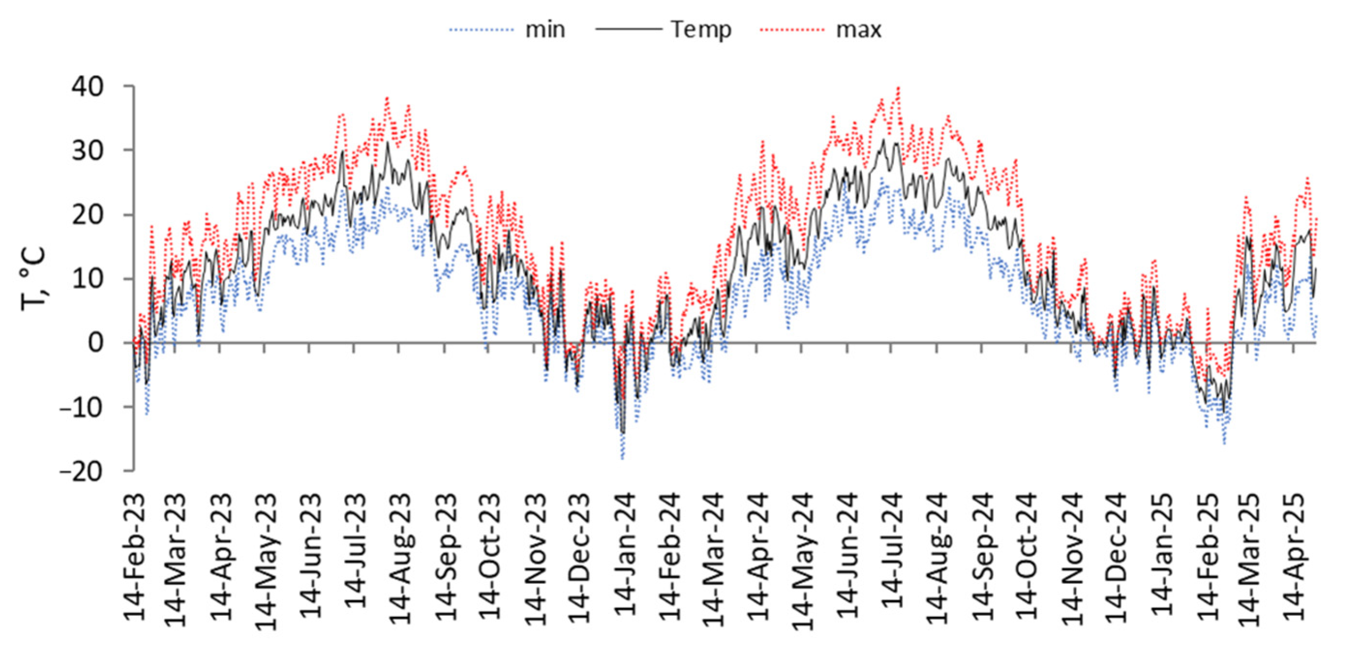
The dynamics of average daily temperatures for the study period are presented in Figure 13.
For woody plants, reaching an average daily temperature of +5 °C is considered a critical threshold for the start of the season [110]. Therefore, MVP was defined as the period from the sustained transition of the average daily air temperature above +5 °C to the decrease in the average daily air temperature below +5 °C.
In 2024, MVP began on 17 April and ended on 21 November. In 2024, MVP began on 24 April and ended on 3 November. In 2025, MVP began on 22 April.

4.3. Object of Study

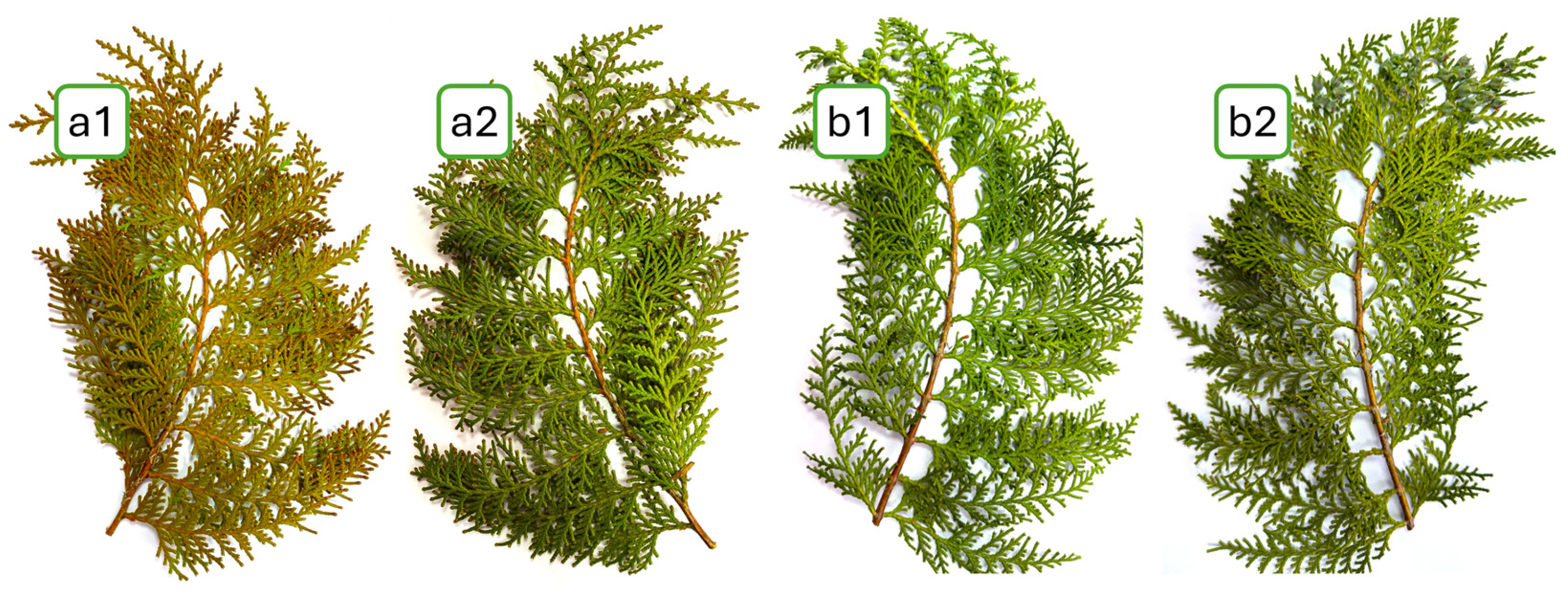
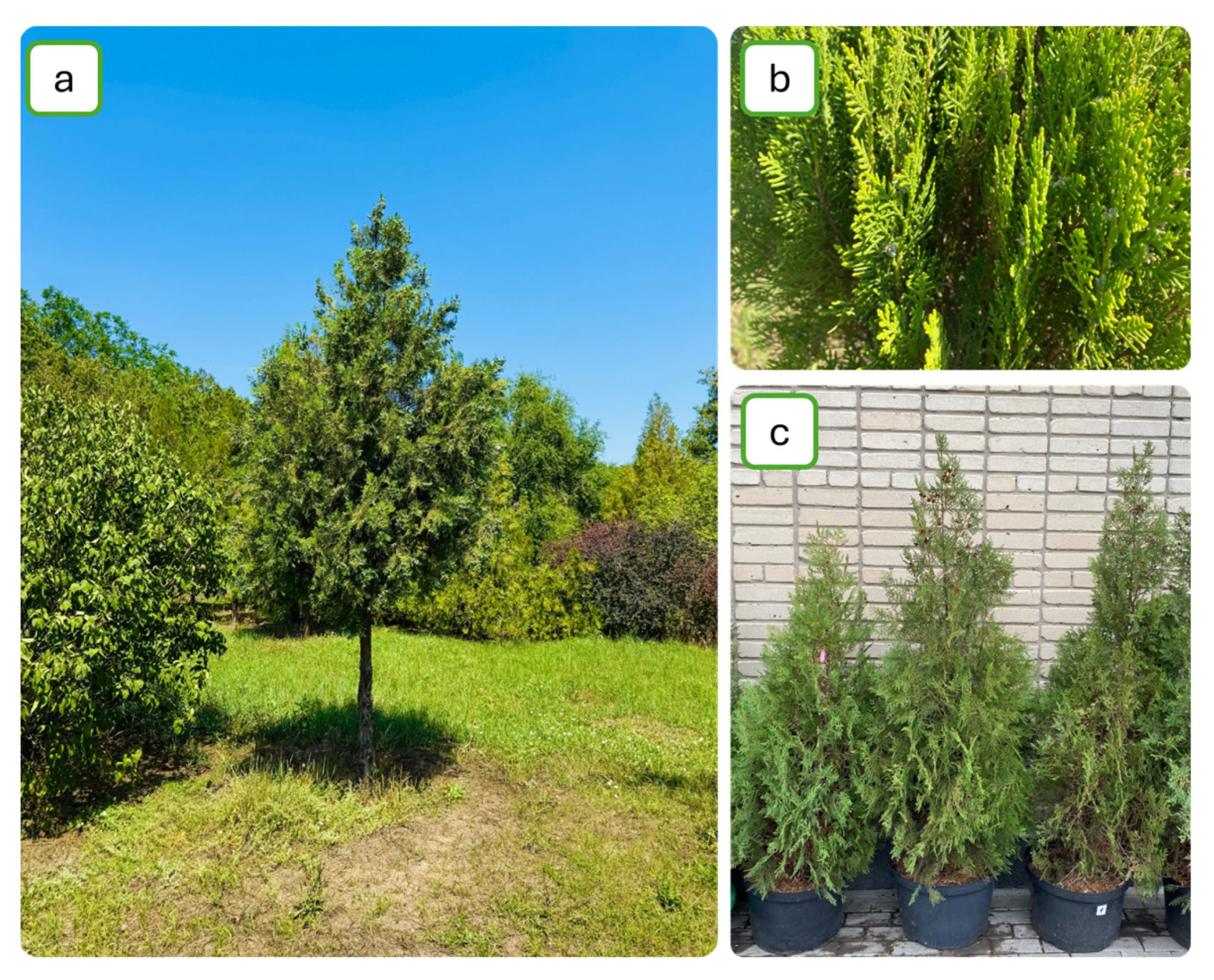
The object of the study was Platycladus orientalis (L.) Franco, an evergreen conifer. This species is native to China and, locally, South Korea. Its needles are scale-like, 1–3 mm long and 0.5–2 mm wide. P. orientalis has been introduced into cultivation in the Rostov Region of Russia. Here, this species exhibits high drought resistance. Its frost resistance is average—young shoots freeze at temperatures below −20 °C. A characteristic feature of P. orientalis is the reversible change in the colour of shoots from green to reddish-brown (Figure 14) during the transition from summer to winter and vice versa. The ‘winter leaf reddening’ effect has been described for other members of the Cupressaceae family and is associated with the accumulation of zeaxanthin of the VAZ cycle, which accumulates in shoots exposed to sunlight [109]. This is an external manifestation of these plants’ response to LS. Figure 14 clearly shows that the ‘winter leaf reddening’ effect is visually detectable only on the illuminated side of the shoot, while the reverse side of the same shoot has a dark green colour. The second characteristic feature of P. orientalis is the vertical rather than horizontal arrangement of the shoots (Figure 15). This protects the needles of P. orientalis from high-intensity sunlight in summer (especially at midday) and is one of its adaptations to arid conditions. However, in winter, when the sun is lower above the horizon, this morphological feature of P. orientalis does not protect it from LS.
The specimens of P. orientalis from which shoots were selected for HSI, determination of photosynthetic pigment content and Fv/Fm values grow in the dendrological collection of the SFedU Botanical Garden under identical conditions, including lighting. The experimental plants are 20–25 years old and are at the generative stage of ontogenesis.
Six-year-old P. orientalis plants (six specimens) planted in technological containers located on the south-facing terrace were used for HSI of the crowns (Figure 15c).

4.4. Sampling of P. orientalis Shoots for Laboratory Research

Shoots for laboratory HSI and determination of photosynthetic pigments were selected from three P. orientalis trees growing in the SFedU Botanical Garden collection. Seven shoots were cut from each tree from the periphery of the crown on the eastern and western sides (Figure 11, V1). The shoots in these parts of the crown were characterised by the fact that the south-facing side of the shoot was maximally exposed to the sun, while the north side of the shoot was constantly in the shade.
Shoots were sampled at intervals of 7–10 days (97 shoot samples were sampled during the entire study period) (Figure 12). The cut shoots were placed in plastic bags and delivered to the laboratory within 30 min. Shoots were selected from P. orientalis specimens contained in containers on the south side (Figure 11, V2) on the dates of laboratory HSI.

4.5. Hyperspectral Imaging Methodology

A Cubert UHD-185 frame camera (Cubert GmbH, Germany) was used for HSI. The camera has a spectral range from 450 to 950 nm and a spectral resolution of 4 nm.
The laboratory HSI covered the period from 14 February 2023 to 28 April 2025. A white reference panel was used to calibrate the reflectance. The experiment was conducted under artificial lighting covering the entire spectral range of the camera. During the HSI, seven shoots of P. orientalis were stacked. With each imaging, the bottom shoot was moved to the top of the stack [65]. The stack of P. orientalis shoots was placed on a black stage, 40 cm from the camera lens. The pixel size at this distance was 0.25 cm2.
Field HSI of P. orientalis crowns was conducted from 29 May to 2 December 2024. The camera was positioned at a distance of 1.7 m from the side of the crown. On all calendar dates, the southern, sunlit side of the P. orientalis crown was imaged.

4.6. Preprocessing of Hyperspectral Imagery Data

The spectral data underwent pre-processing, which included the Savitsky-Golay filter with a step size of 15 nm. A two-step segmentation method was used to select the region of interest (ROI) on the hyperspectral image [63]. In the first stage, the ROI was selected by setting a threshold of Carter5 > 1.4. In the second stage, morphological erosion was applied using a 3 × 3 structuring element. Pixels with ROI were selected using random reverse selection. The spectral profiles of the ROI area on each hyperspectral image were transformed using the Random Reflectance [111].
Twenty-eight VIs were calculated, the abbreviations and formulas of which are presented in Table 1.

4.7. Determination of Photosynthetic Pigment Content

The determination of photosynthetic pigments was carried out in parallel with HSI. To determine the concentrations of photosynthetic pigments, shoots of P. orientalis were used, which were imaged using a hyperspectral camera. The needles were cut from the periphery of these shoots, carefully chopped and mixed. Then, three samples weighing 500 mg each were taken from the resulting mass for pigment extraction. This procedure was performed for each tree. Pigments were extracted in 96% ethanol, as described by Lichtenthaler and Wellburn [112]. The concentration of chlorophyll a (CChl a), chlorophyll b (CChl b) and carotenoids (CCar) (mg/g dry plant material) was determined spectrophotometrically using a Beckman Du 730 (USA) spectrophotometer.

4.8. Measurement of Maximum Quantum Yields of Photosystem II (Fv/Fm)

Fv/Fm measurements were taken between 31 July 2024 and 28 April 2025. The experiment was conducted taking into account the following facts. (1) The optimal Fv/Fm for conifers is approximately 0.800 [20,113,114]. (2) When cut winter shoots of conifers are kept in laboratory conditions at a temperature in the range of +18...+20 °C and low photosynthetic photon flux density (PPFD) (5 to 10 mmol photons m−2s−1), they recover from LS within 24 to 100 h, depending on the calendar date of sampling and the species of conifer [20,113]. (3) During the first two hours after the shoots are transferred to laboratory conditions, the Fv/Fm curve shows a lag phase [113].
In the present study, P. orientalis shoots were placed in darkness for 30 min immediately after delivery to the laboratory. After that, Fv/Fm was measured on the illuminated and shaded sides of the shoot using a DivingPAM fluorometer (Waltz, Effeltrich, Germany). The Fv/Fm was determined at ten different points for each shoot.
The air temperature in the laboratory was maintained at around +20 °C, and the PPFD was 5 mmol photons m−2s−1.

4.9. Data Analytics

Data analysis was performed using standard statistical methods, as well as Principal Component Analysis (PCA) and ML algorithms—RF and Linear Discriminant Analysis (LDA). Data processing was performed in the R (version number 4.5.1.) environment [115].
The randomForest package was used to construct the RF model [116]. A 5-fold cross-validation method was used to adjust the hyperparameters and to assess efficacy. RF hyperparameters: number of trees = 100 and number of variables tried at each split = 5.
The MASS package was used to construct the LDA model [117].
Time series of proximal HSI data of conifers shoots for the period from 14 February 2023 to 18 November 2024 were used for training. Time series of proximal HSI data of conifers shoots for the period from 21 November 2024 to 28 April 2025 and time series of proximal HSI data of conifers canopy for the period from 14 February 2023 to 28 April 2025 were used for testing.
The number of pixels by class was aligned to the minimum value. For each class, it was 18,000.
To assess the multicollinearity of vegetation indices, a correlation matrix and variance inflation factor (VIF) were used. A threshold value of VIF = 5 was taken [118].

5. Limitations of the Study

The manuscript presents preliminary research results. The study aimed to prove the fundamental possibility of recording light stress using HSI. The design of the study did not allow us to classify the states of ‘cold stress’ and ‘optimal condition’ on P. orientalis crowns. The study used only Ccar and Cchl/Ccar -sensitive VIs, which also probably prevented the classification of the ‘cold stress’ and ‘optimal condition’ conditions on the crowns. Hyperspectral imaging of P. orientalis crowns was conducted for one season. At the same time, long-term studies on plant crowns are necessary to construct universal classification models for conifers in MVP and dormancy. The use of equipment for HSI and Fv/Fm determination in field conditions at low sub-zero temperatures presents a technical challenge.

6. Conclusions

The RF algorithm made it possible to classify the states ‘Winter Light Stress’ and ‘Optimal Condition’ with high accuracy. The out-of-bag (OOB) estimate of the error rate was only 0.35%. Classification of the states ‘Cold Stress’ and ‘Optimal Condition’ can also be considered successful, with an OOB error rate estimate of 3.19%. The states ‘Winter Light Stress’ and ‘Cold Stress’ were less well separated, with an OOB estimate of error rate of 15.94%. LDA models showed high accuracy in discriminating between these states (96.7%, 90.4% and 78.6%, respectively). Verifying the RF model for the simultaneous classification of the three conditions (‘Optimal condition’, ‘Cold stress’ and ‘Winter Light Stress’) using field survey data on tree crowns showed that the ‘Winter Light Stress’ condition was identified correctly. At the same time, ‘Optimal condition’ was identified as ‘Cold stress’. The following vegetation indices were significant for identifying WLS: CARI, CCI, CCRI, CRI550, CTRI, LSI, PRI, PRIm1, modPRI and TVI.

Author Contributions

Conceptualization, P.A.D., B.L.K. and V.S.L.; Data curation, B.L.K. and A.A.D.; Formal analysis, A.A.D. and M.M.S.; Investigation, P.A.D., B.L.K. and A.A.D.; Methodology, P.A.D. and B.L.K.; Project administration, P.A.D.; Resources, V.S.L., M.M.S. and T.V.V.; Software, A.A.D.; Writing—original draft, P.A.D. and B.L.K.; Writing—review and editing, P.A.D., B.L.K. and A.A.D. All authors have read and agreed to the published version of the manuscript.

Funding

The project was supported by the Russian Science Foundation under grant No. 22-14-00338-P, https://rscf.ru/project/22-14-00338/ (accessed on 19 October 2025), and performed in Southern Federal University (Rostov-on-Don, Russian Federation).

Data Availability Statement

The original contributions presented in the study are included in the article, further inquiries can be directed to the corresponding author.

Conflicts of Interest

The authors declare no conflicts of interest.

References

  1. Chakhvashvili, E.; Machwitz, M.; Antala, M.; Rozenstein, O.; Prikaziuk, E.; Schlerf, M.; Naethe, P.; Wan, Q.; Komárek, J.; Klouek, T.; et al. Crop stress detection from UAVs: Best practices and lessons learned for exploiting sensor synergies. Precis. Agric. 2024, 25, 2614–2642. [Google Scholar] [CrossRef]
  2. Kashyap, B.; Kumar, R. Sensing Methodologies in Agriculture for Monitoring Biotic Stress in Plants Due to Pathogens and Pests. Inventions 2021, 6, 29. [Google Scholar] [CrossRef]
  3. Kramer, K.; Bouriaud, L.; Feindt, P.H.; van Wassenaer, L.; Glanemann, N.; Hanewinkel, M.; van der Heide, M.; Hengeveld, G.M.; Hoogstra, M.; Ingram, V.; et al. Roadmap to develop a stress test for forest ecosystem services supply. One Earth 2022, 5, 25–34. [Google Scholar] [CrossRef]
  4. Zhang, H.; Zhao, Y.; Zhu, J.-K. Thriving under Stress: How Plants Balance Growth and the Stress Response. Dev. Cell 2020, 55, 529–543. [Google Scholar] [CrossRef]
  5. Yadav, S.; Modi, P.; Dave, A.; Vijapura, A.; Patel, D.; Patel, M. Effect of Abiotic Stress on Crops. In Sustainable Crop Production; IntechOpen: London, UK, 2020. [Google Scholar]
  6. Dey, S.; Raichaudhuri, A. Abiotic Stress in Plants; Intech Open: London, UK, 2022. [Google Scholar] [CrossRef]
  7. Ghosh, P.; Nandi, R.; Das, S.; Roy, A.; Parvin, S.; Dalal, D.; Dalal, D. Plants Response to Abiotic Stress: A Review. Sarcouncil J. Plant Agron. 2023, 1, 1–6. [Google Scholar] [CrossRef]
  8. Liu, M.; Wang, Y.; Zhang, H.; Hao, Y.; Wu, H.; Shen, H.; Zhang, P. Mechanisms of photoprotection in overwintering evergreen conifers: Sustained quenching of chlorophyll fluorescence. Plant Physiol. Biochem. 2024, 210, 108638. [Google Scholar] [CrossRef] [PubMed]
  9. Chang, C.Y.; Bräutigam, K.; Hüner, N.P.A.; Ensminger, I. Champions of winter survival: Cold acclimation and molecular regulation of cold hardiness in evergreen conifers. New Phytol. 2020, 229, 675–691. [Google Scholar] [CrossRef] [PubMed]
  10. Ensminger, I.; Berninger, F.; Streb, P. Response of photosynthesis to low temperature. In Terrestrial Photosynthesis in Achanging Environment: A Molecular, Physiological, and Ecological Approach; Flexas, J., Loreto, F., Medrano, H., Eds.; Cambridge University Press: Cambridge, UK, 2012; pp. 276–293. [Google Scholar]
  11. Öquist, G.; Hüner, N.P.A. Photosynthesis of overwintering evergreen plants. Annu. Rev. Plant Biol. 2003, 54, 329–355. [Google Scholar] [CrossRef] [PubMed]
  12. Crosatti, C.; Rizza, F.; Badeck, F.W.; Mazzucotelli, E.; Cattivelli, L. Harden the chloroplast to protect the plant. Physiol. Plant. 2013, 147, 55–63. [Google Scholar] [CrossRef]
  13. Shavnin, S.A.; Yusupov, I.A.; Marina, N.V.; Montile, A.A.; Golikov, D.Y. Seasonal changes in chlorophyll and carotenoid content in needles of scots pines (Pinus sylvestris L.) Exposed to the thermal field of a gas flare. Russ. J. Plant Physiol. 2021, 68, 526–535. [Google Scholar] [CrossRef]
  14. William, W.A.; Zarter, C.R.; Ebbert, V.; Demmig-Adams, B. Photoprotective Strategies of Overwintering Evergreens. BioScience 2004, 54, 41–49. [Google Scholar] [CrossRef]
  15. Shi, Y.; Ke, X.; Yang, X.; Liu, Y.; Hou, X. Plants response to light stress. J. Genet. Genom. 2022, 49, 735–747. [Google Scholar] [CrossRef] [PubMed]
  16. Zhang, M.; Ming, Y.; Wang, H.-B.; Jin, H.-L. Strategies for adaptation to high light in plants. Abiotech 2024, 5, 381–393. [Google Scholar] [CrossRef] [PubMed]
  17. Szymanska, R.; Slesak, I.; Orzechowska, A.; Kruk, J. Physiological and biochemical responses to high light and temperature stress in plants. Environ. Exp. Bot. 2017, 139, 165–177. [Google Scholar] [CrossRef]
  18. Baránková, B.; Lazár, D.; Nauš, J. Analysis of the effect of chloroplast arrangement on optical properties of green tobacco leaves. Remote Sens. Environ. 2016, 174, 181–196. [Google Scholar] [CrossRef]
  19. Araguirang, G.E.; Richter, A.S. Activation of anthocyanin biosynthesis in high light–what is the initial signal? New Phytol. 2022, 236, 2037–2043. [Google Scholar] [CrossRef]
  20. Ottander, C.; Campbell, D.; Oquist, G. Seasonal changes in photosystem II organisation and pigment composition in Pinus sylvestris. Planta 1995, 197, 176–183. [Google Scholar] [CrossRef]
  21. Zhu, H.; Li, X.; Zhai, W.; Liu, Y.; Gao, Q.; Liu, J.; Ren, L.; Chen, H.; Zhu, Y. Effects of low light on photosynthetic properties, antioxidant enzyme activity, and anthocyanin accumulation in purple pak-choi (Brassica campestris ssp. Chinensis Makino). PLoS ONE 2017, 12, e0179305. [Google Scholar] [CrossRef]
  22. Ruban, A.V. Nonphotochemical chlorophyll fluorescence quenching: Mechanism and effectiveness in protecting plants from photodamage. Plant Physiol. 2016, 170, 1903–1916. [Google Scholar] [CrossRef]
  23. Frechette, E.; Chang, C.Y.; Ensminger, I. Photoperiod and temperature constraints on the relationship between the photochemical reflectance index (PRI) and the light-use efficiency of photosynthesis in Pinus strobus. Tree Physiol. 2016, 36, 311–324. [Google Scholar] [CrossRef]
  24. Latowski, D.; Kuczyґnska, P.; Strzałka, K. Xanthophyll cycle—A mechanism protecting plants against oxidative stress. Redox Rep. 2011, 16, 78–90. [Google Scholar] [CrossRef]
  25. Adams, R.W.W.; Demmig-Adams, B.; Rosenstiel, T.N.; Ebbert, V. Dependence of photosynthesis and energy dissipation activity upon growth form and light environment during the winter. Photosynth. Res. 2001, 67, 51–62. [Google Scholar] [CrossRef]
  26. Sveshnikov, D.; Ensminger, I.; Ivanov, A.G.; Campbell, D.; Lloyd, J.; Funk, C.; Hüner, N.P.A.; Öquist, G. Excitation energy partitioning and quenching during cold acclimation in Scots pine. Tree Physiol. 2006, 26, 325–336. [Google Scholar] [CrossRef]
  27. Busch, F.A. Photorespiration in the context of Rubisco biochemistry, CO2 diffusion and metabolism. Plant J. 2020, 101, 919–939. [Google Scholar] [CrossRef] [PubMed]
  28. Murata, N.; Nishiyama, Y. ATP is a driving force in the repair of photosystem II during photoinhibition. Plant Cell Environ. 2018, 41, 285–299. [Google Scholar] [CrossRef] [PubMed]
  29. Kothari, S.; Schweiger, A.K. Plant spectra as integrative measures of plant phenotypes. J. Ecol. 2022, 110, 2536–2554. [Google Scholar] [CrossRef]
  30. Solovchenko, A.; Shurygin, B.; Nesterov, D.A.; Sorokin, D.V. Towards the synthesis of spectral imaging and machine learning-based approaches for non-invasive phenotyping of plants. Biophys. Rev. 2023, 15, 939–946. [Google Scholar] [CrossRef] [PubMed]
  31. Okyere, F.G.; Cudjoe, D.K.; Virlet, N.; Castle, M.; Riche, A.B.; Greche, L.; Mohareb, F.; Simms, D.; Mhada, M.; Hawkesford, M.J. Hyperspectral Imaging for Phenotyping Plant Drought Stress and Nitrogen Interactions Using Multivariate Modeling and Machine Learning Techniques in Wheat. Remote Sens. 2024, 16, 3446. [Google Scholar] [CrossRef]
  32. Dmitriev, P.A.; Kozlovsky, B.L.; Dmitrieva, A.A.; Varduni, T.V.; Lysenko, V.S. Light Stress Detection in Ficus elastica with Hyperspectral Indices. AgriEngineering 2024, 6, 3297–3311. [Google Scholar] [CrossRef]
  33. Bhargava, A.; Sachdeva, A.; Sharma, K.; Alsharif, M.H.; Uthansakul, P.; Uthansakul, M. Hyperspectral imaging and its applications: A review. Heliyon 2024, 10, 33208. [Google Scholar] [CrossRef]
  34. Akewar, M.; Chandak, M. Hyperspectral Imaging Algorithms and Applications: A Review. TechRxiv. 2024. [Google Scholar] [CrossRef]
  35. Montero, D.; Aybar, C.; Mahecha, M.D.; Martinuzzi, F.; Söchting, M.; Wieneke, S. A standardized catalogue of spectral indices to advance the use of remote sensing in Earth system research. Sci. Data 2023, 10, 197. [Google Scholar] [CrossRef] [PubMed]
  36. Xue, J.; Su, B. Significant Remote Sensing Vegetation Indices: A Review of Developments and Applications. J. Sens. 2017, 2017, 1353691. [Google Scholar] [CrossRef]
  37. César, H.-H.; Goulden, M.L. Plant Traits Help Explain the Tight Relationship between Vegetation Indices and Gross Primary Production. Remote Sens. 2020, 12, 1405. [Google Scholar] [CrossRef]
  38. Farella, M.M.; Barnes, M.L.; Breshears, D.D.; Mitchell, J.; van Leeuwen, W.J.D.; Gallery, R.E. Evaluation of Vegetation Indices and Imaging Spectroscopy to Estimate Foliar Nitrogen across Disparate Biomes. Ecosphere 2022, 13, e3992. [Google Scholar] [CrossRef]
  39. Shumaila, K.; Chandni, Z.; Tayyaba, R.; Sara, A.; Aimen, A.; Bushra, A.; Mujahid, A. The significance of chlorophylls and carotenoids in enhancing seed tolerance to abiotic stress. Biol. Clin. Sci. Res. J. 2024, 5, 1081. [Google Scholar] [CrossRef]
  40. Zhou, X.; Huang, W.; Zhang, J.; Kong, W.; Casa, R.; Huang, Y. A novel combined spectral index for estimating the ratio of carotenoid to chlorophyll content to monitor crop physiological and phenological status. Int. J. Appl. Earth Obs. Geoinf. 2019, 76, 128–142. [Google Scholar] [CrossRef]
  41. He, C.; Sun, J.; Chen, Y.; Wang, L.; Shi, S.; Qiu, F.; Tagesson, T. A new vegetation index combination for leaf carotenoid-to-chlorophyll ratio: Minimizing the effect of their correlation. Int. J. Digit. Earth 2023, 16, 272–288. [Google Scholar] [CrossRef]
  42. Wang, H.; Shi, R.; Liu, P.D.; Gao, W. Dual NDVI Ratio Vegetation Index: A Kind of Vegetation Index Assessing Leaf Carotenoid Content Based on Leaf Optical Properties Model. Guang Pu Xue Yu Guang Pu Fen Xi 2016, 36, 2189–2194. [Google Scholar] [CrossRef]
  43. Gitelson, A.A.; Zygielbaum, A.I.; Arkebauer, T.J.; Walter-Shea, E.A.; Solovchenko, A. Stress detection in vegetation based on remotely sensed light absorption coefficient. Int. J. Remote Sens. 2024, 45, 259–277. [Google Scholar]
  44. Chappelle, E.W.; Kim, M.S.; McMurtrey, J.E., III. Ratio analysis of reflectance spectra (RARS): An algorithm for the remote estimation of the concentrations of chlorophyll a, chlorophyll b, and carotenoids in soybean leaves. Remote Sens. Environ. 1992, 39, 239–247. [Google Scholar] [CrossRef]
  45. Blackburn, G.A. Spectral indices for estimating photosynthetic pigment concentrations: A test using senescent tree leaves. Int. J. Remote Sens. 1998, 19, 657–675. [Google Scholar] [CrossRef]
  46. Gitelson, A.A.; Zur, Y.; Chivkunova, O.B.; Merzlyak, M.N. Assessing Carotenoid Content in Plant Leaves with Reflectance Spectroscopy. Photochem. Photobiol. 2002, 75, 272–281. [Google Scholar] [CrossRef]
  47. Gitelson, A.A.; Keydan, G.P.; Merzlyak, M.N. Three-band model for noninvasive estimation of chlorophyll, carotenoids, and anthocyanin contents in higher plant leaves. Geophys. Res. Lett. 2006, 33, L11402. [Google Scholar] [CrossRef]
  48. Zhou, X.; Wenjiang, H.; Weiping, K.; Huichun, Y.; Yingying, D.; Raffaele, C. Assessment of leaf carotenoids content with a new carotenoid index: Development and validation on experimental and model data. Int. J. Appl. Earth Obs. Geoinf. 2017, 57, 24–35. [Google Scholar] [CrossRef]
  49. Weiping, K.; Huang, W.; Zhou, X.; Song, X.; Casa, R. Estimation of carotenoid content at the canopy scale using the carotenoid triangle ratio index fromin situand simulated hyperspectral data. J. Appl. Remote Sens. 2016, 10, 026035. [Google Scholar] [CrossRef]
  50. Gamon, J.A.; Penuelas, J.; Field, C.B. A narrow-waveband spectral index that tracks diurnal changes in photosynthetic efficiency. Remote Sens. Environ. 1992, 41, 35–44. [Google Scholar] [CrossRef]
  51. Broge, N.H.; Leblanc, E. Comparing prediction power and stability of broadband and hyperspectral vegetation indices for estimation of green leaf area index and canopy chlorophyll density. Remote Sens. Environ. 2001, 76, 156–172. [Google Scholar] [CrossRef]
  52. Haboudane, D.; Miller, J.R.; Tremblay, N.; Zarco-Tejada, P.J.; Dextraze, L. Integrated narrow-band vegetation indices for prediction of crop chlorophyll content for application to precision agriculture. Remote Sens. Environ. 2002, 81, 416–426. [Google Scholar] [CrossRef]
  53. Hernandez-Clemente, R.; Navarro-Cerrillo, R.M.; Suбrez, L.; Morales, F.; Zarco-Tejada, P.J. Assessing structural effects on PRI for stress detection in conifer forests. Remote Sens. Environ. 2011, 115, 2360–2375. [Google Scholar] [CrossRef]
  54. Hernandez-Clemente, R.; Navarro-Cerrillo, R.M.; Zarco-Tejada, P.J. Carotenoid content estimation in a heterogeneous conifer forest using narrowband indices and PROSPECT + DART simulations. Remote Sens. Environ. 2012, 127, 298–315. [Google Scholar] [CrossRef]
  55. Haboudane, D. Hyperspectral vegetation indices and novel algorithms for predicting green LAI of crop canopies: Modeling and validation in the context of precision agriculture. Remote Sens. Environ. 2004, 90, 337–352. [Google Scholar] [CrossRef]
  56. Datt, B. Remote Sensing of Chlorophyll a, Chlorophyll b, Chlorophyll a+b, and Total Carotenoid Content in Eucalyptus Leaves. Remote Sens. Environ. 1998, 66, 111–121. [Google Scholar] [CrossRef]
  57. Chen, S.; Kosugi, Y.; Jiao, L.; Sakabe, A.; Epron, D.; Nakaji, T.; Noda, H.; Hikosaka, K.; Nasahara, K.N. Winter leaf reddening and photoprotection accessed by vegetation indices and its influence on canopy light-use efficiency of a Japanese cypress (Chamaecyparis obtusa) forest. Agric. For. Meteorol. 2025, 363, 110427. [Google Scholar] [CrossRef]
  58. Escadafal, R.; Huete, A. Etude des propriétés spectrales des sols arides appliquée à l′amélioration des indices de végétation obtenus par télédétection. Comptes Rendus L′Académie Sci. 1991, 312, 1385–1391. [Google Scholar]
  59. Gitelson, A. Towards a generic approach to remote non-invasive estimation of foliar carotenoid-tochlorophyll ratio. J. Plant Physiol. 2020, 252, 153227. [Google Scholar] [CrossRef]
  60. Yang, F.; Li, J.; Gan, X.; Qian, Y.; Wu, X.; Yang, Q. Assessing nutritional status of Festuca arundinacea by monitoring photosynthetic pigments from hyperspectral data. Comput. Electron. Agric. 2010, 70, 52–59. [Google Scholar] [CrossRef]
  61. Gamon, J.A.; Huemmrich, K.F.; Wong, C.Y.; Ensminger, I.; Garrity, S.; Hollinger, D.Y.; Noormets, A.; Penuelas, J. A remotely sensed pigment index reveals photosynthetic phenology in evergreen conifers. Proc. Natl. Acad. Sci. USA 2016, 113, 13087–13092. [Google Scholar] [CrossRef]
  62. Penuelas, J.; Baret, F.; Filella, I. Semi-empirical indices to assess carotenoids/chlorophyll a ratio from leaf spectral reflectance. Photosynthetica 1995, 31, 221–230. [Google Scholar]
  63. Dmitriev, P.A.; Kozlovsky, B.L.; Dmitrieva, A.A.; Lysenko, V.S.; Chokheli, V.A.; Varduni, T.V. Indication of Light Stress in Ficus elastica Using Hyperspectral Imaging. AgriEngineering 2023, 5, 2253–2265. [Google Scholar] [CrossRef]
  64. Dmitriev, P.A.; Kozlovsky, B.L.; Dmitrieva, A.A. Assessing the phenological state of evergreen conifers using hyperspectral imaging time series. Remote Sens. Appl. Soc. Environ. 2024, 36, 101342. [Google Scholar] [CrossRef]
  65. Guo, J.; Liu, X.; Ge, W.; Zhao, L.; Fan, W.; Zhang, X.; Lu, Q.; Xing, X.; Zhou, Z. Tracking photosynthetic phenology using spectral indices at the leaf and canopy scales in temperate evergreen and deciduous trees. Agric. For. Meteorol. 2024, 344, 109809. [Google Scholar] [CrossRef]
  66. Sasagawa, T.; Akitsu, T.K.; Ide, R.; Takagi, K.; Takanashi, S.; Nakaji, T.; Nasahara, K.N. Accuracy Assessment of Photochemical Reflectance Index (PRI) and Chlorophyll Carotenoid Index (CCI) Derived from GCOM-C/SGLI with In Situ Data. Remote Sens. 2022, 14, 5352. [Google Scholar] [CrossRef]
  67. Gamon, J.; Serrano, L.; Surfus, J. The photochemical reflectance index: An optical indicator of photosynthetic radiation use efficiency across species, functional types, and nutrient levels. Oecologia 1997, 112, 492–501. [Google Scholar] [CrossRef] [PubMed]
  68. Rakgoale, P.B.; Ngetar, S.N. Detecting Invasive Alien Plant Species Using Remote Sensing, Machine Learning and Deep Learning. J. Sens. 2024, 23, 8854675. [Google Scholar] [CrossRef]
  69. Grewal, R.; Singh Kasana, S.; Kasana, G. Machine Learning and Deep Learning Techniques for Spectral Spatial Classification of Hyperspectral Images: A Comprehensive Survey. Electronics 2023, 12, 488. [Google Scholar] [CrossRef]
  70. Swe, K.N.; Noguchi, N. Comparison of machine learning and deep learning models for the assessment of rondo wine grape quality with a hyperspectral camera. Smart Agric. Technol. 2024, 8, 100474. [Google Scholar] [CrossRef]
  71. Saha, D.; Manickavasagan, A. Machine learning techniques for analysis of hyperspectral images to determine quality of food products: A review. Curr. Res. Food Sci. 2021, 4, 28–44. [Google Scholar] [CrossRef]
  72. Dmitriev, P.A.; Kozlovsky, B.L.; Dmitrieva, A.A. Vegetation and Dormancy States Identification in Coniferous Plants Based on Hyperspectral Imaging Data. Horticulturae 2024, 10, 241. [Google Scholar] [CrossRef]
  73. Ma, J.; Chen, X.; Han, F.; Song, Y.; Zhou, B.; Nie, Y.; Li, Y.; Niu, S. The long road to bloom in conifers. For. Res. 2022, 2, 16. [Google Scholar] [CrossRef]
  74. Röhrig, E.; Ulrich, B. Temperate deciduous forests. Ecosyst. World 1991, 7, 557–558. [Google Scholar]
  75. Thomas, S.C.; MacLellan, J. Boreal and Temperate Forests. For. For. Plants 2009, 1, 152. [Google Scholar]
  76. Vankat, J. Boreal and Temperate Forests. Encycl. Life Sci. 2002. [Google Scholar] [CrossRef]
  77. Venäläinen, A.; Lehtonen, I.; Laapas, M.; Ruosteenoja, K.; Tikkanen, O.P.; Viiri, H.; Ikonen, V.P.; Peltola, H. Climate change induces multiple risks to boreal forests and forestry in Finland: A literature review. Glob. Change Biol. 2020, 26, 4178–4196. [Google Scholar] [CrossRef] [PubMed]
  78. Zhang, X.; Manzanedo, R.; Xu, G.; Lapenis, A.G. Editorial: Achieving sustainable development goal 13: Resilience and adaptive capacity of temperate and boreal forests under climate change. Front. For. Glob. Change 2024, 7, 1356686. [Google Scholar] [CrossRef]
  79. Sheikh, M.A.; Tiwari, A.; Anjum, J.; Sharma, S. Dynamics of carbon storage and status of standing vegetation in temperate coniferous forest ecosystem of north western Himalaya India. Vegetos 2021, 34, 822–833. [Google Scholar] [CrossRef]
  80. Zhang, Q.; Luan, R.; Wang, M.; Zhang, J.; Yu, F.; Ping, Y.; Qiu, L. Research Progress of Spectral Imaging Techniques in Plant Phenotype Studies. Plants 2024, 13, 3088. [Google Scholar] [CrossRef]
  81. Cotrozzi, L. Spectroscopic detection of forest diseases: A review (1970–2020). J. For. Res. 2022, 33, 21–38. [Google Scholar] [CrossRef]
  82. Paul, N.; Sunil, G.C.; Horvath, D.; Sun, X. Deep learning for plant stress detection: A comprehensive review of technologies, challenges, and future directions. Comput. Electron. Agric. 2025, 229, 109734. [Google Scholar] [CrossRef]
  83. Ye, D.; Wu, L.; Li, X.; Atoba, T.O.; Wu, W.; Weng, H. A Synthetic Review of Various Dimensions of Non-Destructive Plant Stress Phenotyping. Plants 2023, 12, 1698. [Google Scholar] [CrossRef]
  84. Williams, D.; Karley, A.; Britten, A.; McCallum, S.; Graham, J. Raspberry plant stress detection using hyperspectral imaging. Plant Direct 2023, 7, e490. [Google Scholar] [CrossRef] [PubMed]
  85. Blackburn, G.A. Hyperspectral remote sensing of plant pigments. J. Exp. Bot. 2007, 58, 855–867. [Google Scholar] [CrossRef] [PubMed]
  86. Yan, K.; Gao, S.; Yan, G.; Ma, X.; Chen, X.; Zhu, P.; Li, J.; Gao, S.; Gastellu-Etchegorry, J.-P.; Myneni, R.B.; et al. A global systematic review of the remote sensing vegetation indices. Int. J. Appl. Earth Obs. Geoinf. 2025, 139, 104560. [Google Scholar] [CrossRef]
  87. Wong, C.Y.S. Plant optics: Underlying mechanisms in remotely sensed signals for phenotyping applications. AoB Plants 2023, 15, plad039. [Google Scholar] [CrossRef]
  88. Ashraf, M.; Harris, P.J.C. Photosynthesis under stressful environments: An overview. Photosynthetica 2013, 51, 163–190. [Google Scholar] [CrossRef]
  89. Sun, Y.; Qin, Q.; Zhang, Y.; Ren, H.; Han, G.; Zhang, Z.; Zhang, T.; Wang, B. A leaf chlorophyll vegetation index with reduced LAI effect based on Sentinel-2 multispectral red-edge information. Comput. Electron. Agric. 2025, 236, 110500. [Google Scholar] [CrossRef]
  90. Cheshkova, A.F. A review of hyperspectral image analysis techniques for plant disease detection and identification. Vavilovskii Zhurnal Genet. I Sel. Vavilov J. Genet. Breed. 2022, 26, 202–213. [Google Scholar] [CrossRef]
  91. Wan, L.; Li, H.; Li, C.; Wang, A.; Yang, Y.; Wang, P. Hyperspectral Sensing of Plant Diseases: Principle and Methods. Agronomy 2022, 12, 1451. [Google Scholar] [CrossRef]
  92. Poblete, T.; Watt, M.S.; Buddenbaum, H.; Zarco-Tejada, P.J. Chlorophyll content estimation in radiata pine using hyperspectral imagery: A comparison between empirical models, scaling-up algorithms, and radiative transfer inversions. Agric. For. Meteorol. 2025, 362, 110402. [Google Scholar] [CrossRef]
  93. Mertens, S.; Verbraeken, L.; Sprenger, H.; Demuynck, K.; Maleux, K.; Cannoot, B.; De Block, J.; Maere, S.; Nelissen, H.; Bonaventure, G.; et al. Proximal Hyperspectral Imaging Detects Diurnal and Drought-Induced Changes in Maize Physiology. Front. Plant Sci. 2021, 12, 640914, Erratum in Front. Plant Sci. 2024, 15, 1379654. [Google Scholar] [CrossRef]
  94. Misra, G.; Cawkwell, F.; Wingler, A. Status of Phenological Research Using Sentinel-2 Data: A Review. Remote Sens. 2020, 12, 2760. [Google Scholar] [CrossRef]
  95. Zeng, L.; Wardlow, B.D.; Xiang, D.; Hu, S.; Li, D. A Review of Vegetation Phenological Metrics Extraction Using Time-Series, Multispectral Satellite Data. Remote Sens. Environ. 2020, 237, 111511. [Google Scholar] [CrossRef]
  96. Berra, E.F.; Gaulton, R. Remote sensing of temperate and boreal forest phenology: A review of progress, challenges and opportunities in the intercomparison of in-situ and satellite phenological metrics. For. Ecol. Manag. 2021, 480, 118663. [Google Scholar] [CrossRef]
  97. Dronova, I.; Taddeo, S. Remote sensing of phenology: Towards the comprehensive indicators of plant community dynamics from species to regional scales. J. Ecol. 2022, 110, 1460–1484. [Google Scholar] [CrossRef]
  98. Lu, B.; Dao, P.D.; Liu, J.; He, Y.; Shang, J. Recent Advances of Hyperspectral Imaging Technology and Applications in Agriculture. Remote Sens. 2020, 12, 2659. [Google Scholar] [CrossRef]
  99. Mishra, P.; Lohumi, S.; Haris, A.K.; Nordon, A. Close-range hyperspectral imaging of whole plants for digital phenotyping: Recent applications and illumination correction approaches. Comput. Electron. Agric. 2020, 178, 105780. [Google Scholar] [CrossRef]
  100. Han, Q.; Wang, T.; Jiang, Y.; Fischer, R.; Li, C. Phenological variation decreased carbon uptake in European forests during 1999–2013. For. Ecol. Manag. 2018, 427, 45–51. [Google Scholar] [CrossRef]
  101. Schrodt, F.; de la Barreda Bautista, B.; Williams, C.; Boyd, D.S.; Schaepman-Strub, G.; Santos, M.J. Integrating biodiversity, remote sensing, and auxiliary information for the study of ecosystem functioning and conservation at large spatial scales. In Remote Sensing of Plant Biodiversity; Springer International Publishing: Berlin/Heidelberg, Germany, 2020; pp. 449–484. [Google Scholar] [CrossRef]
  102. Wang, X.; Zhou, Y.; Wen, R.; Zhou, C.; Xu, L.; Xi, X. Mapping Spatiotemporal Changes in Vegetation Growth Peak and the Response to Climate and Spring Phenology over Northeast China. Remote Sens. 2020, 12, 3977. [Google Scholar] [CrossRef]
  103. Lebrini, Y.; Boudhar, A.; Laamrani, A.; Htitiou, A.; Lionboui, H.; Salhi, A.; Chehbouni, A.; Benabdelouahab, T. Mapping and Characterization of Phenological Changes over Various Farming Systems in an Arid and Semi-Arid Region Using Multitemporal Moderate Spatial Resolution Data. Remote Sens. 2021, 13, 578. [Google Scholar] [CrossRef]
  104. Denny, E.G.; Gerst, K.L.; Miller-Rushing, A.J.; Tierney, G.L.; Crimmins, T.M.; Enquist, C.A.F.; Guertin, P.; Rosemartin, A.H.; Schwartz, M.D.; Thomas, K.A.; et al. Standardized phenology monitoring methods to track plant and animal activity for science and resource management applications. Int. J. Biometeorol. 2014, 58, 591–601. [Google Scholar] [CrossRef]
  105. Vyse, K.; Pagter, M.; Zuther, E.; Hincha, D.K. Deacclimation after cold acclimation—A crucial, but widely neglected part of plant winter survival. J. Exp. Bot. 2019, 70, 4595–4604. [Google Scholar] [CrossRef]
  106. Weiser, C.J. Cold Resistance and Injury in Woody Plants. Science 1970, 169, 1269–1278. [Google Scholar] [CrossRef] [PubMed]
  107. Beck, E.H.; Heim, R.; Hansen, J. Plant resistance to cold stress: Mechanisms and environmental signals triggering frost hardening and dehardening. J. Biosci. 2004, 29, 449–459. [Google Scholar] [CrossRef] [PubMed]
  108. Seyednasrollah, B.; Bowling, D.R.; Cheng, R.; Logan, B.A.; Magney, T.S.; Frankenberg, C.; Yang, J.C.; Young, A.M.; Hufkens, K.; Arain, M.A.; et al. Seasonal variation in the canopy color of temperate evergreen conifer forests. New Phytol. 2021, 229, 2586–2600. [Google Scholar] [CrossRef]
  109. Ida, K. Eco-physiological studies on the response of taxodiaceous conifers to shading, with special reference to the behaviour of leaf pigments—I. Distribution of carotenoids in green and autumnal reddish brown leaves of gymnosperms. Bot. Mag. 1981, 94, 41–54. [Google Scholar] [CrossRef]
  110. Körner, C.; Möhl, P.; Hiltbrunner, E. Four ways to define the growing season. Ecol. Lett. 2023, 26, 1277–1292. [Google Scholar] [CrossRef]
  111. Dmitriev, P.A.; Dmitrieva, A.A.; Kozlovsky, B.L. Random Reflectance: A New Hyperspectral Data Preprocessing Method for Improving the Accuracy of Machine Learning Algorithms. AgriEngineering 2025, 7, 90. [Google Scholar] [CrossRef]
  112. Lichtenthaler, H.K.; Wellburn, A.R. Determinations of total carotenoids and chlorophylls a and b of leaf extracts in different solutionts. Biochem. Soc. Trans. 1983, 11, 591–592. [Google Scholar] [CrossRef]
  113. Verhoeven, A. Recovery kinetics of winter stressed conifers: The effects of growth light environment, extent of the season, and species. Nat Prec. 2010. [Google Scholar] [CrossRef]
  114. Nippert, J.B.; Duursma, R.A.; Marshall, J.D. Seasonal variation in photosynthetic capacity of montane conifers. Funct. Ecol. 2004, 18, 876–886. [Google Scholar] [CrossRef]
  115. R Core Team. R: A Language and Environment for Statistical Computing; R Foundation for Statistical Computing: Vienna, Austria, 2025; Available online: https://www.R-project.org/ (accessed on 9 August 2025).
  116. Liaw, A.; Wiener, M. Classification and Regression by Random Forest. R News 2002, 2, 18–22. [Google Scholar]
  117. Venables, W.N.; Ripley, B.D. Modern Applied Statistics with S, 4th ed.; Springer: New York, NY, USA, 2002. [Google Scholar]
  118. Zuur, A.F.; Ieno, E.N.; Elphick, C.S. A protocol for data exploration to avoid common statistical problems. Methods Ecol. Evol. 2010, 1, 3–14. [Google Scholar] [CrossRef]
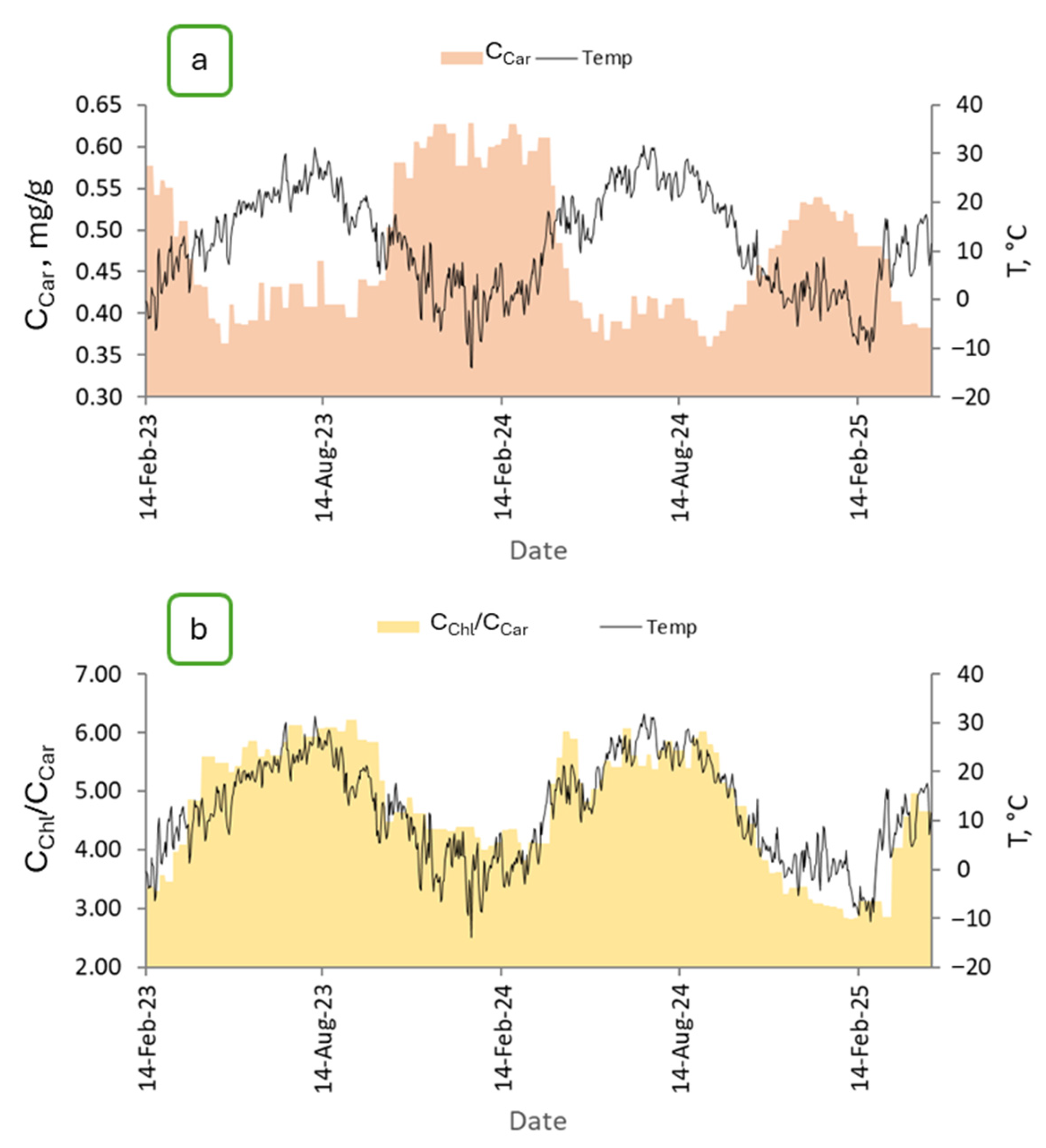
Figure 1. The dynamics of CCar (a) and Cchl/Ccar (b) in the shoots of Platycladus orientalis illuminated by the sun relative to the dynamics of the average daily air temperature.
Stresses 05 00062 g001
Figure 2. CCar (a) and Cchl/Ccar (b) regressions in Platycladus orientalis shoots illuminated by the sun from the average daily air temperature for the period from 14 February 2023 to 17 April 2025.
Stresses 05 00062 g002
Figure 3. Dynamics of Fv/Fm in comparison with the dynamics of CCar (a) and Cchl/Ccar (b) shoots of Platycladus orientalis.
Stresses 05 00062 g003
Figure 4. Regressions of the Fv/Fm values of Platycladus orientalis shoots from CCar (a,c) and Cchl/Ccar (b,d) for the period from 31 July 2024 to 28 April 2025.
Stresses 05 00062 g004
Figure 5. Matrix of pairwise coefficients of determination for the values of vegetation indices. The results are based on the entire two-year time series of spectral characteristics of the shoots of Platycladus orientalis illuminated by the sun. The symbol ‘Χ’ indicates the absence of a significant correlation. The red frame indicates groups of VIs obtained as a result of hierarchical clustering.
Stresses 05 00062 g005
Figure 6. The results of the evaluation of the spectral state of Platycladus orientalis shoots under cold stress, winter light stress and optimal condition using principal component analysis (PCA). (a)—Lighted and shaded sides of the shoot under optimal conditions (vegetation period); (b)—shaded side of the shoot under optimal conditions and under cold stress; (c)—sunlit side of the shoot under optimal conditions and under light stress; (d)—sunlit side of the shoot under light stress and shaded side of the shoot under cold stress.
Stresses 05 00062 g006
Figure 7. The significance of VIs for RF classification by their contribution to the values of Mean Decrease Accuracy and Mean Decrease Gini. (a)—‘Winter Light Stress’ and ‘Optimal condition’; (b)—‘Cold stress’ and ‘Optimal condition’; (c)—‘Winter Light Stress’ and ‘Cold stress’; (d)—‘Winter Light Stress’, ‘Cold stress’ and ‘Optimal condition’.
Stresses 05 00062 g007
Figure 8. Discrimination of “Winter Light Stress”, “Cold stress” and “Optimal condition” of Platycladus orientalis shoots.
Stresses 05 00062 g008
Figure 9. The results of the random forest (RF) classification of the winter light stress (WLS) shoots of Platycladus orientalis in comparison with the average daily air temperatures. The fraction of escape pixels classified as WLS is presented.
Stresses 05 00062 g009
Figure 10. The results of testing the random forest (RF) model for the possibility of predicting the conditions ‘Optimal condition’, ‘Cold stress’ and ‘Winter Light Stress’: (a)—crowns; (b)—shoots.
Stresses 05 00062 g010
Figure 11. Sampling sites (V1 and V2) of shoots from the crown of Platycladus orientalis (top view).
Stresses 05 00062 g011
Figure 12. Details of the timing of Platycladus orientalis shoot selection, hyperspectral imaging and measurement of physiological characteristics.
Stresses 05 00062 g012
Figure 13. Dynamics of average daily temperatures during the study.
Stresses 05 00062 g013
Figure 14. Winter (a) and summer (b) shoots of Platycladus orientalis. The side of the shoot exposed to the sun (1) and the side of the same shoot in the shade (2).
Stresses 05 00062 g014
Figure 15. Appearance of Platycladus orientalis (a), shoot arrangement (b), container culture of Platycladus orientalis (c).
Stresses 05 00062 g015
Table 1. Vegetation indices for assessing Ccar, Cchl/Ccar and light stress.
Vegetation IndexFormulaReference
Ccar VIs
RARScR760/R500[44]
PSSRcR800/R470[45]
PSNDc(R800 − R470)/(R800 + R470)[45]
CRI550R510–1 − R550−1[46]
CRI700R510–1 − R700−1[46]
CARred-edge(R510−1 − R700−1) × R770[47]
CARgreen(R510−1 − R550−1) × R770[47]
CARI(R720 − R521)/R521[48]
CTRI[1.2 × [1.2 × (R800 − R550) − 2.5 × (R670 − R550)]]/R531[49]
PRI(R531 − R570)/(R531 + R570)[50]
TVI0.5 × [120 × (R750 − R550) − 200 × (R670 − R480)][51]
TCARI3 × [(R700 − R670) − 0.2 × (R700 − R550) × (R700/R670)][52]
PRIm1(R512 − R531)/(R512 + R531)[53]
SRcarR515/R570[54]
MTVI11.2 × [1.2 × (R800 − R550) − 2.5 × (R670 − R550)][55]
Datt4R672/(R550 × R708)[56]
RI(R470 − R540)/(R470 + R540)[57,58]
Cchl/Ccar VIs
CCRI = CARI/CIred-edge[(R720 − R521)/R521]/(R750 − R705)/R705[40]
(α500/α700) − 1[(R800/R500)/(R800/R700)] − 1[59]
α500 − α660(R800/R500) − (R800/R660)[59]
RVIR761/R738[60]
CCI(R528 − R645)/(R528 + R645)[61]
CTRI/CIred-edge[[1.2 × [1.2 × (R800 − R550) − 2.5 × (R670 − R550)]]/R531]/[(R750 − R705)/R705][41]
SIPI(R800 − R445)/(R800 + R680)[62]
LS VIs
modPRI515/550(R515 − R550)/(R515 + R550)[43]
LSImean(R666:682)/mean(R552:594)[63]
LSIRedR674/R654[32]
LSINorm(R674 − R654)/(R674 + R654)[32]
Table 2. The variance inflation factor (VIF) for vegetation indices (VI) used in modelling winter light stress.
VIVIFVIVIFVIVIF
CCRI4.10LSI2.16Datt41.51
CRI7003.88TCARI1.96PRIm11.45
PRI3.52CTRI1.73LSINorm1.45
CARI3.16RARSc1.66LSIRed1.43
CCI3.13CARgreen1.66RVI1.42
a7002.87MTVI11.64SIPI1.40
SRcar2.53a6601.57RI1.39
CARrededge2.51modPRI1.56PSNDc1.13
CRI5502.48TVI1.56PSSRc1.10
Table 3. Confusion matrix pixel-based random forest (RF) classification of Platycladus orientalis shoot states in various combinations.
GroupStateWinter Light StressOptimal ConditionCold StressClass. Error, %OOB Estimate of Error Rate, %
‘Winter Light Stress’ & ‘Optimal condition’Winter Light Stress17,93862-0.30.35
Optimal condition6417,936-0.4
‘Cold stress’ & ‘Optimal condition’Cold stress-56317,4373.13.19
Optimal condition-17,4155853.3
‘Winter Light Stress’ & ‘Cold stress’Cold stress3346-14,65418.615.94
Winter Light Stress15,606-239413.3
‘Winter Light Stress’ & ‘Cold stress’ & ‘Optimal condition’Cold stress14,147323961421.412.8
Winter Light Stress247715,5121113.8
Optimal condition562717,4313.2
Table 4. Results of discrimination of Platycladus orientalis shoot states using linear discriminant analysis (LDA).
Combination of StatesDiscrimination EquationsCorrectness Rate, %
«Winter Light Stress» and «Optimal condition»LD1 = 0.722 × CCI − 0.749 × CCRI + 0.567 × PRI − 0.670 × PRIm196.7
«Cold stress» and «Optimal condition»LD1 = 0.349 × CRI550 − 0.470 × CARI − 0.704 × CCRI − 0.395 × modPRI − 0.369 × PRIm1 − 0.384 × TVI90.4
«Winter Light Stress» and «Cold stress»LD1 = − 0.667 × CCI + 0.460 × CCRI − 0.359 × LSIRed − 0.449 × PRI + 0.320 × PRIm179.9
«Winter Light Stress» and «Cold stress» and «Optimal condition»LD1 = 0.486 × CCI − 0.748 × CCRI − 0.421 × modPRI + 0.443 × PRI − 0.459 × PRIm1 − 0.220 × TVI
LD2 = 0.818 × CCI − 0.312 × CCRI − 0.265 × modPRI + 0.300 × PRI − 0.106 × PRIm1 − 0.834 × TVI
78.6
Disclaimer/Publisher’s Note: The statements, opinions and data contained in all publications are solely those of the individual author(s) and contributor(s) and not of MDPI and/or the editor(s). MDPI and/or the editor(s) disclaim responsibility for any injury to people or property resulting from any ideas, methods, instructions or products referred to in the content.