

Influence of Coarse Material on the Yield Strength and Viscosity of Debris Flows


Abstract
1. Introduction
2. Previous Work
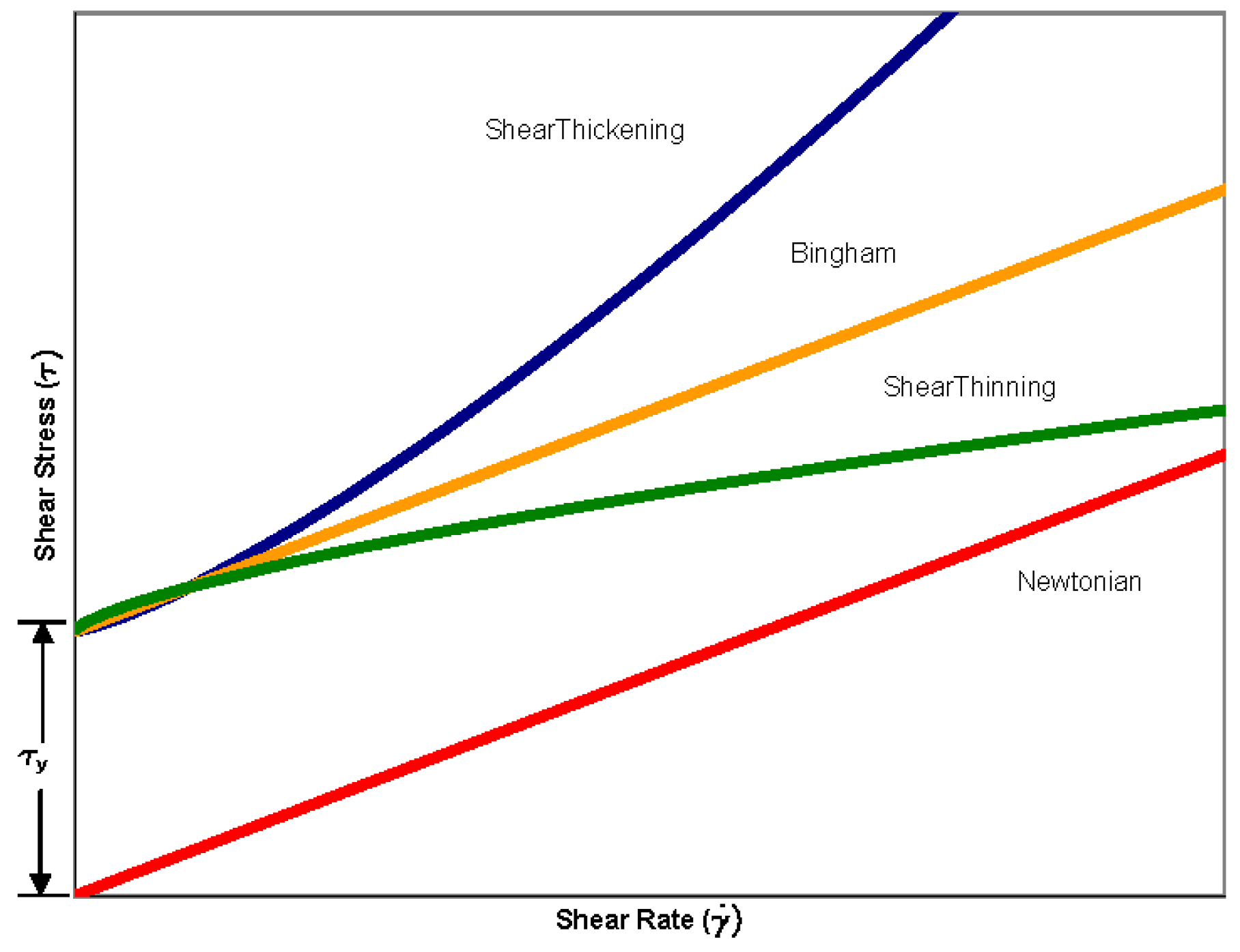
2.1. Debris-Flow Rheology
2.2. Laboratory Experimental Methods
3. Methods
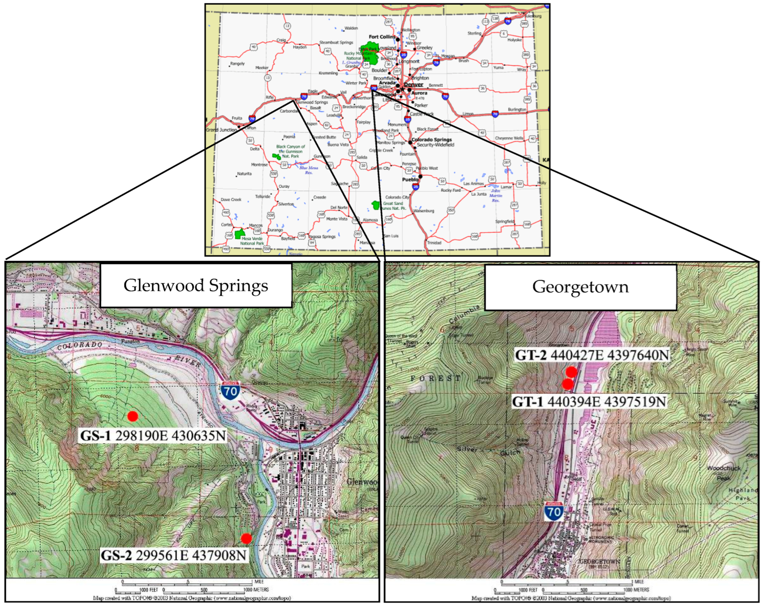
3.1. Sample Collection
3.2. Laboratory Tests of Yield Strength and Viscosity
3.3. Rolling Sleeve Viscometer Methodology

| Latex Sleeve | 6-mil Plastic Sleeve 31.1 cm Circumference | 4-mil Plastic Sleeve 71.1 cm Circumference | |
|---|---|---|---|
| Shear stress correction (°) (is) | 1 | 5 | 2.5 |
| Viscosity correction (Pa-s) () | 0.24 | 2.57 | 5.40 |
3.4. Slump Test Methodology
4. Results
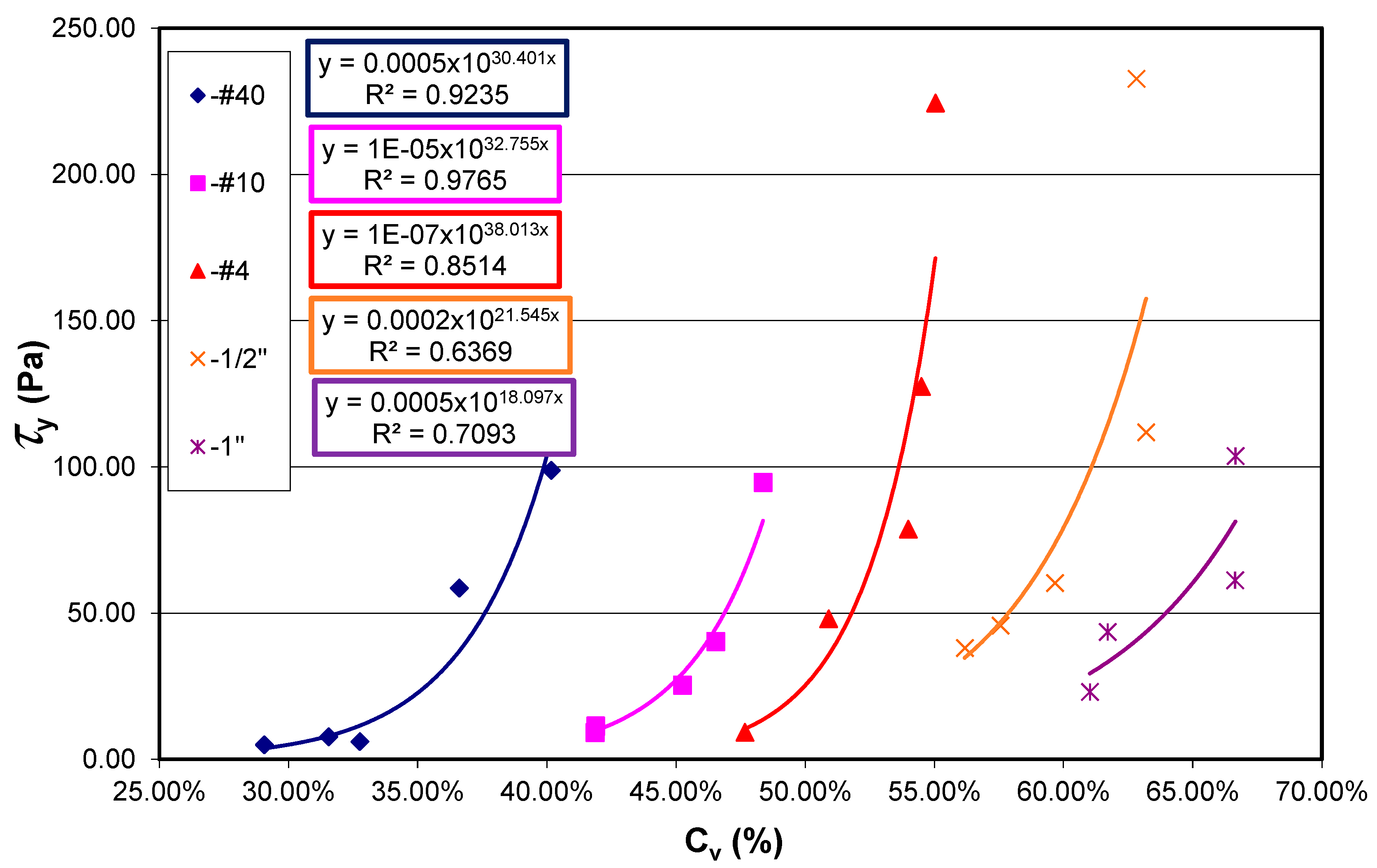
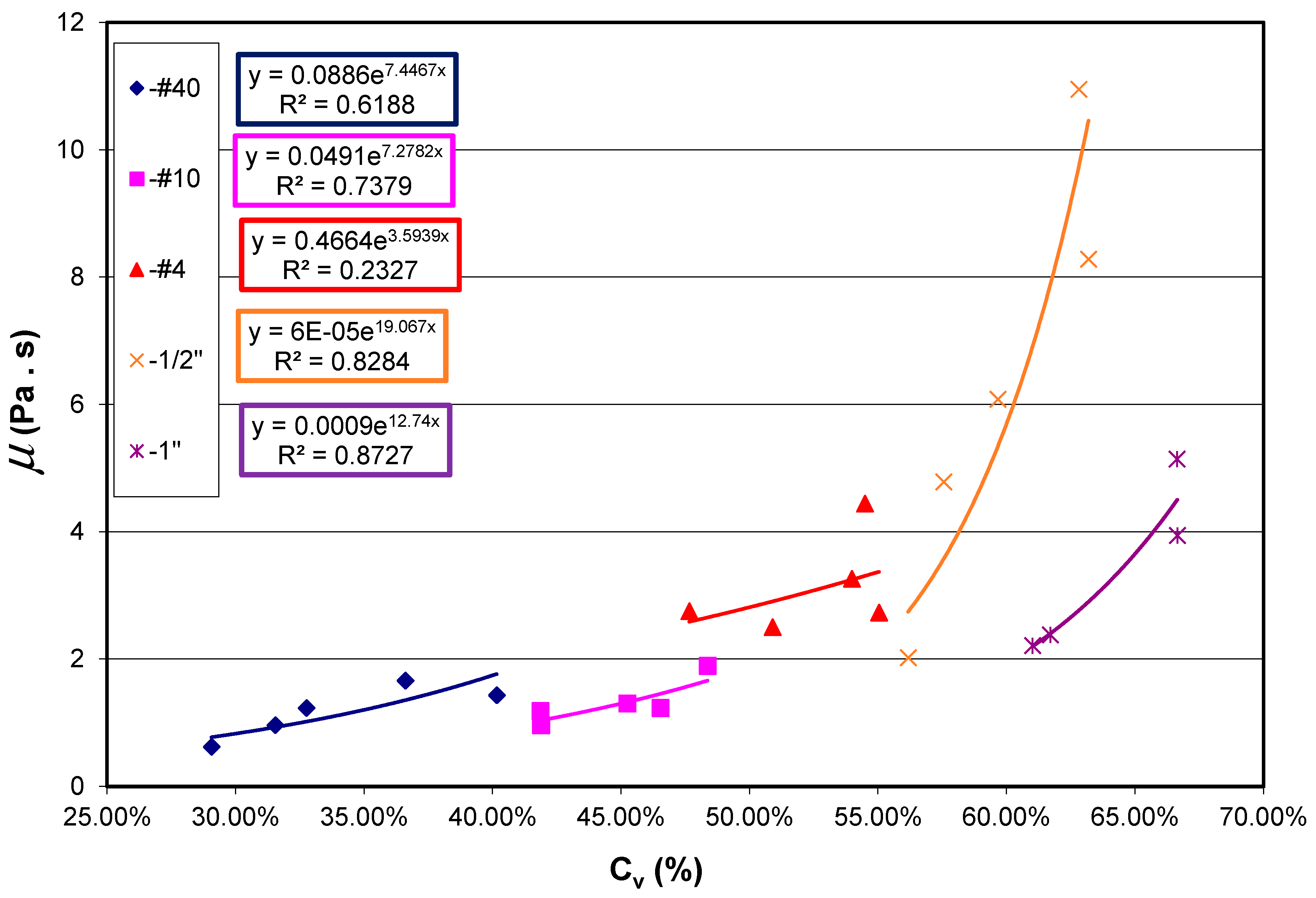
| Yield Strength (Pa) | Viscosity (Pa.s) | ||||||
|---|---|---|---|---|---|---|---|
| τy = α1eβ1Cv | μ = α2eβ2Cv | ||||||
| Sample | dmax (mm) | α1 | β1 | R2 | α2 | β2 | R2 |
| GT-1 | 0.43 | ND | ND | ND | ND | ||
| 2.00 | ND | ND | ND | ND | |||
| 4.75 | ND | ND | ND | ND | |||
| 12.70 | ND | ND | ND | ND | |||
| 25.40 | ND | ND | ND | ND | |||
| GT-2 | 0.43 | 5.00 × 10⁻⁴ | 30.40 | 0.91 | 8.86 × 10⁻² | 7.45 | 0.71 |
| 2.00 | 1.00 × 10⁻⁵ | 32.76 | 0.98 | 4.91 × 10⁻² | 7.28 | 0.72 | |
| 4.75 | 1.00 × 10⁻⁷ | 38.01 | 0.94 | 6.00 × 10⁻⁵ | 19.07 | 0.84 | |
| 12.70 | 2.00 × 10⁻⁴ | 21.55 | 0.82 | 4.66 × 10⁻¹ | 3.59 | 0.24 | |
| 25.40 | 2.00 × 10⁻⁴ | 18.10 | 0.77 | 9.00 × 10⁻⁴ | 12.74 | 0.93 | |
| GS-1 | 0.43 | 2.79 × 10⁻² | 21.97 | 0.82 | 1.15 × 10⁻¹ | 5.86 | 0.40 |
| 2.00 | 1.69 × 10⁻² | 20.29 | 0.92 | 1.73 × 10⁻² | 10.35 | 0.78 | |
| 4.75 | 1.78 × 10⁻² | 19.71 | 0.91 | 2.59 × 10 | −0.91 | 0.01 | |
| 12.70 | 7.31 × 10⁻¹ | 10.00 | 0.86 | 3.20 × 10⁻¹ | 5.08 | 0.75 | |
| 25.40 | 2.00 × 10⁻¹⁰ | 50.14 | 0.99 | 5.03 × 10 | −1.08 | 0.04 | |
| GS-2 | 0.43 | 1.72 × 10 | 16.01 | 0.98 | 1.46 × 10⁻¹ | 8.12 | 0.69 |
| 2.00 | 1.38 × 10⁻¹ | 23.38 | 0.99 | 4.57 × 10⁻¹ | 2.61 | 0.18 | |
| 4.75 | 5.97 × 10⁻¹ | 17.02 | 1.00 | 4.21 × 10 | −2.54 | 0.32 | |
| 12.70 | 5.42 × 10 | 7.75 | 0.94 | 2.52 × 10 | 0.11 | 0.00 | |
| 25.40 | 7.00 × 10⁻³ | 22.73 | 0.98 | 4.34 × 10 | 1.78 | 0.19 | |
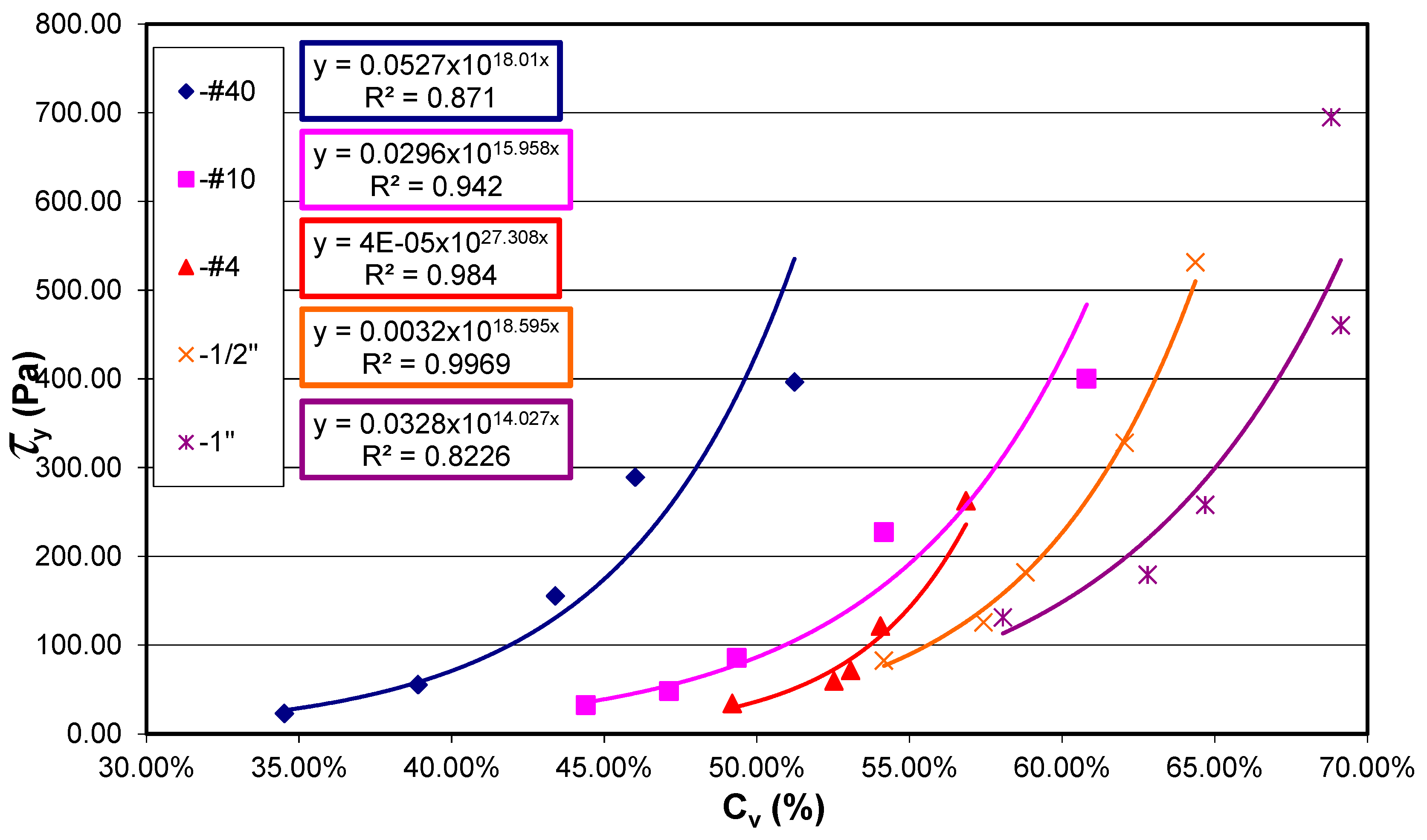
| Yield Strength (Pa) | ||||
|---|---|---|---|---|
| τy = α1eβ1Cv | ||||
| Sample | dmax (mm) | α1 | β1 | R2 |
| GT-1 | 0.43 | 3.57 × 10 | 8.15 | 0.94 |
| 2.00 | 2.84 × 10 | 7.38 | 0.93 | |
| 4.75 | 1.19 × 101 | 5.79 | 1.00 | |
| 12.70 | NR | NR | ||
| 25.40 | NR | NR | ||
| GT-2 | 0.43 | 5.27 × 10⁻² | 18.01 | 0.96 |
| 2.00 | 2.96 × 10⁻² | 15.96 | 0.96 | |
| 4.75 | 4.00 × 10⁻⁵ | 27.31 | 0.95 | |
| 12.70 | 3.20 × 10⁻³ | 19.60 | 0.99 | |
| 25.40 | 3.28 × 10⁻² | 14.03 | 0.90 | |
| GS-1 | 0.43 | 1.52 × 10⁻¹ | 17.56 | 1.00 |
| 2.00 | 5.50 × 10⁻² | 17.84 | 0.97 | |
| 4.75 | 8.40 × 10⁻³ | 21.28 | 1.00 | |
| 12.70 | 5.20 × 10⁻³ | 21.53 | 0.91 | |
| 25.40 | 3.83 × 10⁻² | 15.31 | 0.78 | |
| GS-2 | 0.43 | 3.01 × 10 | 13.97 | 1.00 |
| 2.00 | 2.08 × 10 | 13.51 | 0.99 | |
| 4.75 | 2.99 × 10 | 11.11 | 0.99 | |
| 12.70 | 1.35 × 10⁻¹ | 17.28 | 0.92 | |
| 25.40 | 4.60 × 10⁻³ | 22.80 | 0.84 | |
5. Discussion
5.1. Test Data
5.2. Rolling Sleeve Viscometer
5.3. Slump Test
5.4. Comparison of Test Results to Published Values
5.5. Proposed Method for Yield Stress Curve Prediction
- Step 1—Determine yield strength as a function of sediment concentration curves
- Step 2—Calculate sediment concentrations for a given yield strength
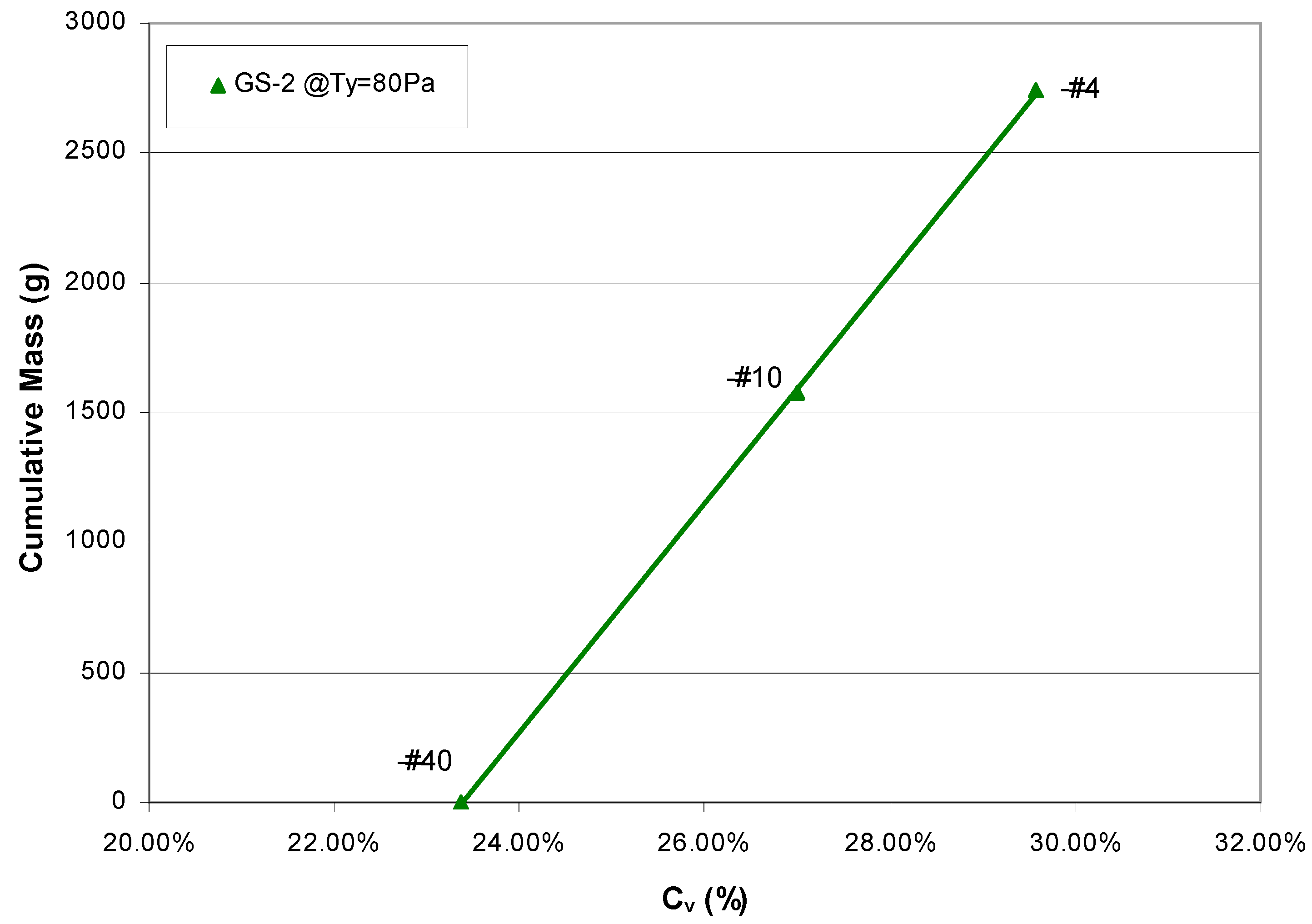
- Step 3—Plot the cumulative mass versus sediment concentration line
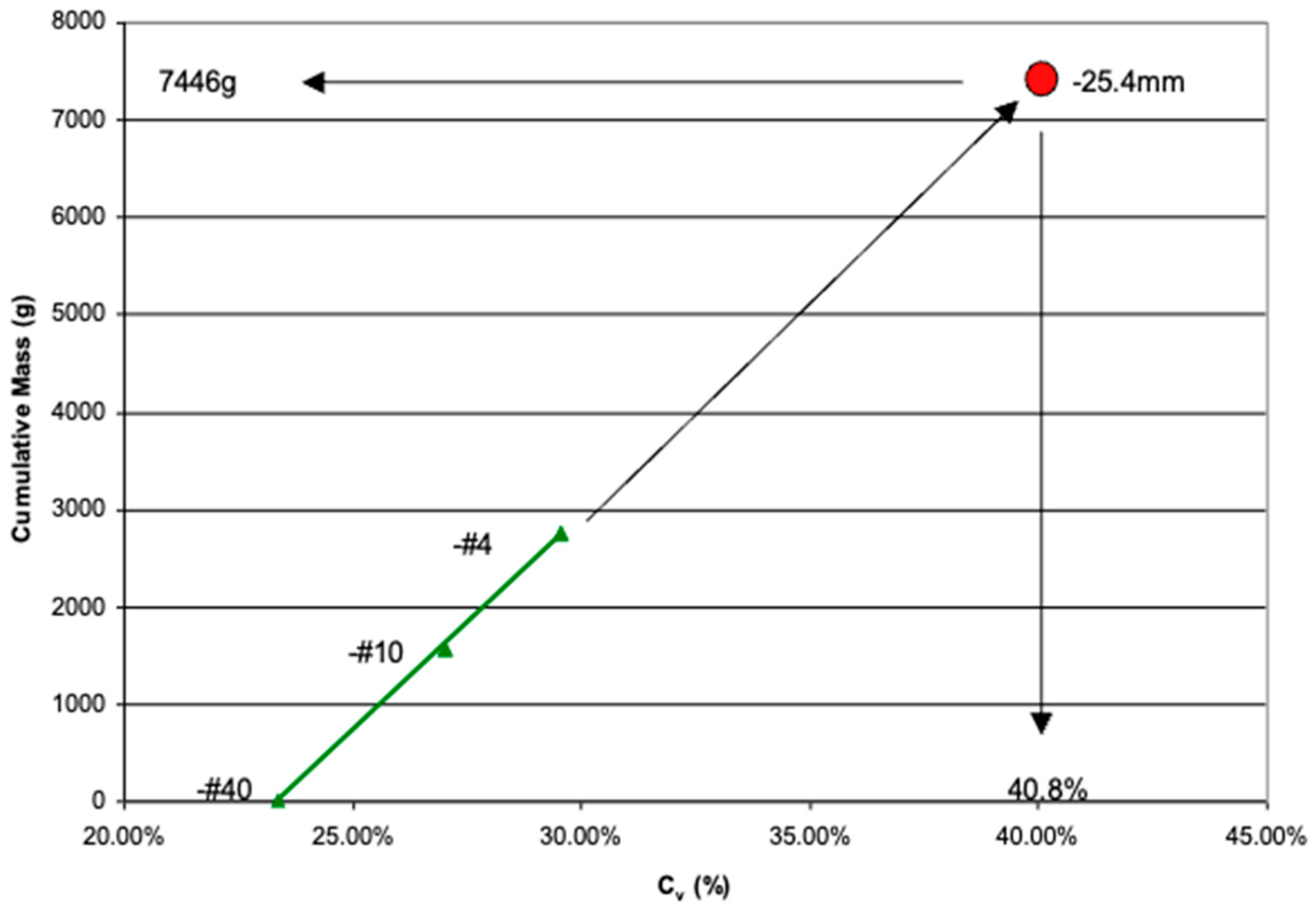
- Step 4—Predict the yield strength step-over for the desired grain size distribution
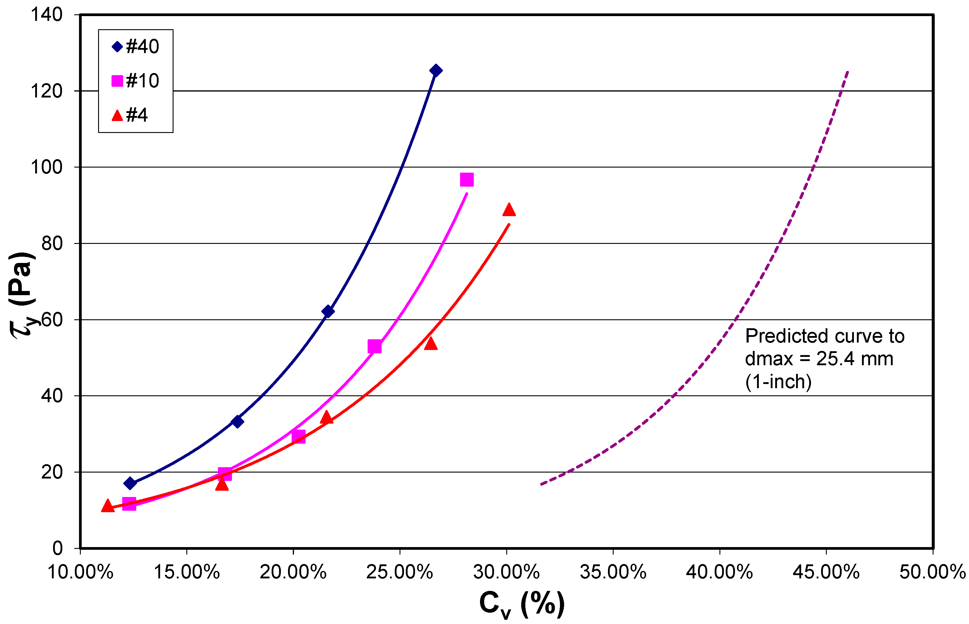
- Step 5—Plot the predicted yield strength versus sediment concentration curve
5.6. Viscosity Prediction
6. Conclusions
- The study confirms that both the yield strength and viscosity plotted as functions of sediment concentration of a slurry follow an exponential regression trend.
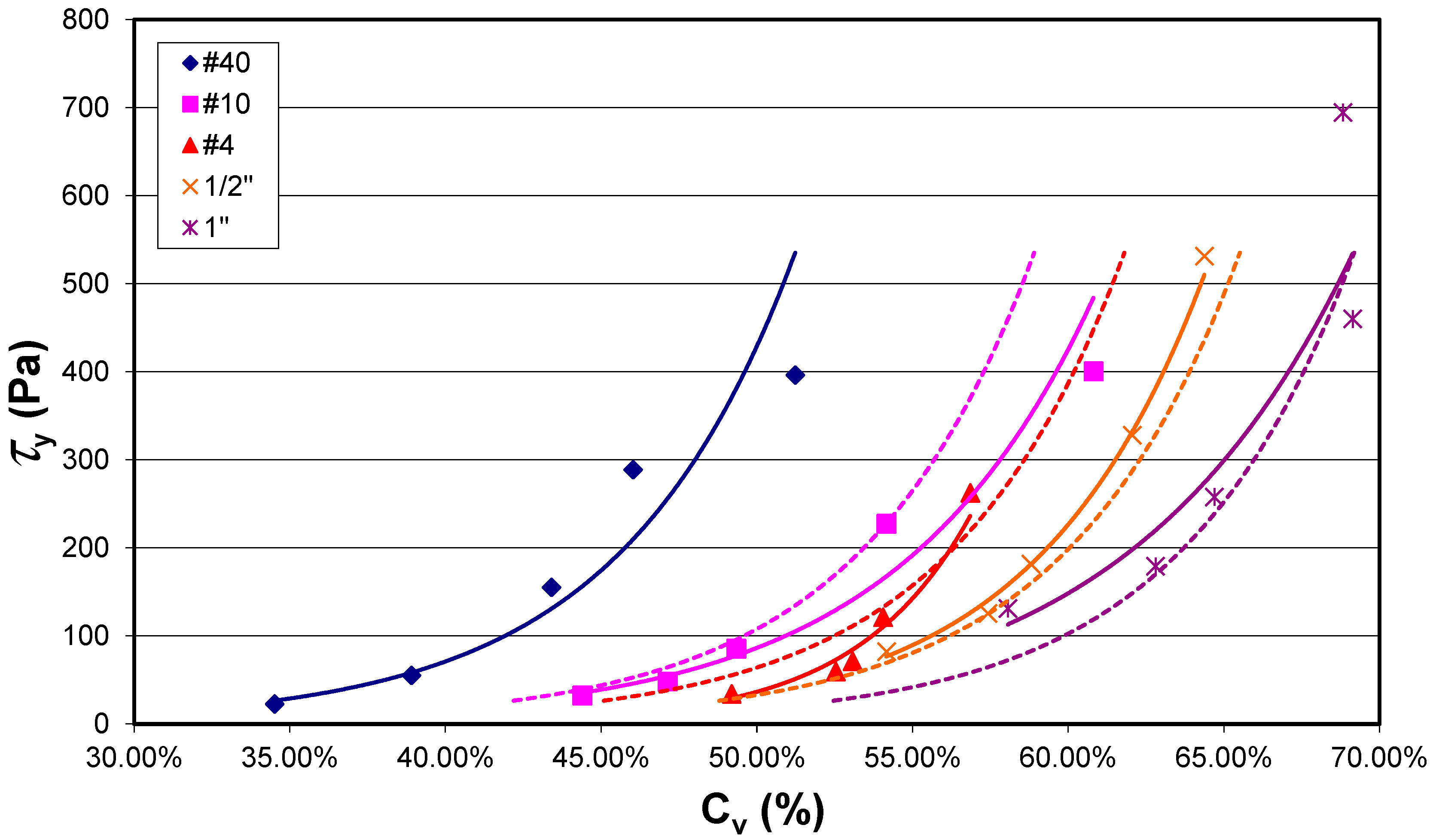
- The addition of progressively larger particles increases the sediment concentration at which a given yield strength is achieved. The addition creates a step-over in the yield strength but the shape of the regression curve remains essentially unchanged.
- It appears that the addition of coarse particles affects the viscosity of the material, through the change in sediment concentration. The variation in viscosity can be predicted by sediment concentration alone without knowing the exact grain size distribution.
- Four laboratory tests were evaluated. The flume box and inclined plane tests were found to produce either highly scattered data, results that were largely inconsistent with other tests, or both. The slump test was recommended as the best of the four tests for determining yield strength when large particles (dmax > 12.7 mm) are present in the sample. Test results for viscosity are on the low end of the range reported in a selection of published values in the technical literature, but yield strength values are comparable.
- Methods for the prediction of both yield strength from a reduced portion of a complete grain size distribution were proposed. The method for yield strength as a function of sediment concentration prediction provides satisfactory results, accurate to within about 25% of the original data, which is within the margin of error for the tests.
- Prediction of viscosity is more straightforward than for yield strength because the grain size distribution is not a controlling factor. Prediction of viscosity is dependent on the test and equipment used, and for this study is accurate to within about 100% at the largest particle sizes tested.
Author Contributions
Funding
Data Availability Statement
Conflicts of Interest
References
- Johnson, A.M.; Rodine, J. Debris Flow. In Slope Instability; Wiley: New York, NY, USA, 1984; pp. 257–361. [Google Scholar]
- Prochaska, A.B.; Santi, P.M.; Higgins, J.D.; Cannon, S.H. A Study of Methods to Estimate Debris Flow Velocity. Landslides 2008, 5, 431–444. [Google Scholar] [CrossRef]
- McCoy, K.; Krasko, V.; Santi, P.; Kaffine, D.; Rebennack, S. Minimizing Economic Impacts from Post-Fire Debris Flows in the Western United States. Nat. Hazards 2016, 83, 149–176. [Google Scholar] [CrossRef]
- Besso, C.; Pereira de Campos, T.M. Laboratory Determination of the Viscosity of Soils for Debris Flow Analysis. In Geotechnical Engineering in the XXI Century: Lessons Learned and Future Challenges; IOS Press: Amsterdam, The Netherlands, 2019; pp. 47–55. [Google Scholar]
- Coussot, P.; Laigle, D.; Arattano, M.; Deganutti, A.; Marchi, L. Direct Determination of Rheological Characteristics of Debris Flow. J. Hydraul. Eng. 1998, 124, 865–868. [Google Scholar] [CrossRef]
- Pashias, N.; Boger, D.V.; Summers, J.; Glenister, D.J. A Fifty Cent Rheometer for Yield Stress Measurement. J. Rheol. 1996, 40, 1179–1189. [Google Scholar] [CrossRef]
- Phillips, C.J.; Davies, T.R.H. Determining Rheological Parameters of Debris Flow Material. Geomorphology 1991, 4, 101–110. [Google Scholar] [CrossRef]
- Coussot, P. Mudflow Rheology and Dynamics; Routledge: London, UK, 2017. [Google Scholar]
- Yano, K.; Daido, A. Fundamental Study on Mud-Flow. Bull. Disaster Prev. Res. Inst. 1965, 14, 69–83. [Google Scholar]
- Johnson, A.M. 1970: Physical Processes in Geology; Freeman Cooper.: San Francisco, CA, USA, 1970; 577p. [Google Scholar]
- Kang, Z.; Zhang, S. A Preliminary Analysis of the Characteristics of Debris-Flow. In Proceedings of the International Symposium of River Sedimentation—Chinese Society for Hydraulic Engineering, Beijing, China, 24–29 March 1980; pp. 225–226. [Google Scholar]
- Major, J.J.; Pierson, T.C. Debris Flow Rheology: Experimental Analysis of Fine-grained Slurries. Water Resour. Res. 1992, 28, 841–857. [Google Scholar] [CrossRef]
- Ballesteros-Cánovas, J.A.; Stoffel, M.; de Haas, T.; Bodoque, J.M. Debris Flow Dating and Magnitude Reconstruction. In Advances in Debris-Flow Science and Practice; Springer: Berlin/Heidelberg, Germany, 2024; pp. 219–248. [Google Scholar]
- Iverson, R.M.; George, D.L. Numerical Modeling of Debris Flows: A Conceptual Assessment. In Advances in Debris-Flow Science and Practice; Springer: Berlin/Heidelberg, Germany, 2024; pp. 127–163. [Google Scholar]
- O’Brien, J.S.; Julien, P.Y.; Fullerton, W.T. Two-Dimensional Water Flood and Mudflow Simulation. J. Hydraul. Eng. 1993, 119, 244–261. [Google Scholar] [CrossRef]
- Chen, H.X.; Zhang, L.M. EDDA 1.0: Integrated Simulation of Debris Flow Erosion, Deposition and Property Changes. Geosci. Model Dev. 2015, 8, 829–844. [Google Scholar] [CrossRef]
- Shen, P.; Zhang, L.; Chen, H.; Fan, R. EDDA 2.0: Integrated Simulation of Debris Flow Initiation and Dynamics Considering Two Initiation Mechanisms. Geosci. Model Dev. 2018, 11, 2841–2856. [Google Scholar] [CrossRef]
- He, J.; Zhang, L.; Fan, R.; Zhou, S.; Luo, H.; Peng, D. Evaluating Effectiveness of Mitigation Measures for Large Debris Flows in Wenchuan, China. Landslides 2022, 19, 913–928. [Google Scholar] [CrossRef]
- Choi, C.E.; Ng, C.W.W.; Liu, H. Flume Modeling of Debris Flows. In Advances in Debris-Flow Science and Practice; Springer: Berlin/Heidelberg, Germany, 2024; pp. 93–125. [Google Scholar]
- Pierson, T.C.; Scott, K.M. Downstream Dilution of a Lahar: Transition from Debris Flow to Hyperconcentrated Streamflow. Water Resour. Res. 1985, 21, 1511–1524. [Google Scholar] [CrossRef]
- O’Brien, J.S. Physical Processes, Rheology and Modeling of Mud Flows (Hyperconcentration, Sediment Flow); Colorado State University: Fort Collins, CO, USA, 1986. [Google Scholar]
- Parsons, J.D.; Whipple, K.X.; Simoni, A. Experimental Study of the Grain-Flow, Fluid-Mud Transition in Debris Flows. J. Geol. 2001, 109, 427–447. [Google Scholar] [CrossRef]
- Jeong, S.W. Grain Size Dependent Rheology on the Mobility of Debris Flows. Geosci. J. 2010, 14, 359–369. [Google Scholar] [CrossRef]
- Schippa, L. The Effects of Sediment Size and Concentration on the Rheological Behavior of Debris Flows. In Granularity in Materials Science; IntechOpen: London, UK, 2018. [Google Scholar]
- Hungr, O. Analysis of Debris Flow Surges Using the Theory of Uniformly Progressive Flow. Earth Surf. Process. Landforms J. Br. Geomorphol. Res. Gr. 2000, 25, 483–495. [Google Scholar] [CrossRef]
- Coussot, P.; Piau, J.-M. The Effects of an Addition of Force-Free Particles on the Rheological Properties of Fine Suspensions. Can. Geotech. J. 1995, 32, 263–270. [Google Scholar] [CrossRef]
- Coussot, P.; Piau, J. A Large-scale Field Coaxial Cylinder Rheometer for the Study of the Rheology of Natural Coarse Suspensions. J. Rheol. 1995, 39, 105–124. [Google Scholar] [CrossRef]
- Schatzmann, M. Rheometry for Large Particle Fluids and Debris Flows; ETH Zurich: Zürich, Switzerland, 2005. [Google Scholar]
- Schippa, L. Modeling the Effect of Sediment Concentration on the Flow-like Behavior of Natural Debris Flow. Int. J. Sediment Res. 2020, 35, 315–327. [Google Scholar] [CrossRef]
- Johnson, A.M. A Model for Debris Flow; The Pennsylvania State University: University Park, PA, USA, 1965. [Google Scholar]
- Hungr, O.; Morgan, G.C.; Kellerhals, R. Quantitative Analysis of Debris Torrent Hazards for Design of Remedial Measures. Can. Geotech. J. 1984, 21, 663–677. [Google Scholar] [CrossRef]
- Takahashi, T. Unified Dynamics of the Inertial Debris Flows. In Proceedings of the 28th IAHR World Congress, Graz, Austria, 22–27 August 1999. [Google Scholar]
- Major, J.J. Gravity-Driven Consolidation of Granular Slurries: Implications for Debris-Flow Deposition and Deposit Characteristics. J. Sediment. Res. 2000, 70, 64–83. [Google Scholar] [CrossRef]
- Iverson, R.M. The Debris-Flow Rheology Myth. Debris-Flow Hazards Mitig. Mech. Predict. Assess. 2003, 1, 303–314. [Google Scholar]
- Rickenmann, D. Empirical Relationships for Debris Flows. Nat. Hazards 1999, 19, 47–77. [Google Scholar] [CrossRef]
- VanDine, D.F. Debris Flow Control Structures for Forest Engineering. Br. Columbia Minist. For. Res. Program Work. Pap. 1996, 8, 1996. [Google Scholar]
- Brighenti, R.; Segalini, A.; Ferrero, A.M. Debris Flow Hazard Mitigation: A Simplified Analytical Model for the Design of Flexible Barriers. Comput. Geotech. 2013, 54, 1–15. [Google Scholar] [CrossRef]
- Kostynick, R.; Matinpour, H.; Pradeep, S.; Haber, S.; Sauret, A.; Meiburg, E.; Dunne, T.; Arratia, P.; Jerolmack, D. Rheology of Debris Flow Materials Is Controlled by the Distance from Jamming. Proc. Natl. Acad. Sci. USA 2022, 119, e2209109119. [Google Scholar] [CrossRef]
- Major, J.J.; Iverson, R.M. Debris-Flow Deposition: Effects of Pore-Fluid Pressure and Friction Concentrated at Flow Margins. Geol. Soc. Am. Bull. 1999, 111, 1424–1434. [Google Scholar] [CrossRef]
- Coussot, P.; Boyer, S. Determination of Yield Stress Fluid Behaviour from Inclined Plane Test. Rheol. Acta 1995, 34, 534–543. [Google Scholar] [CrossRef]
- Rickenmann, D.; Weber, D. Flow Resistance of Natural and Experimental Debris-Flows in Torrent Channels. In Debris-Flow Hazards Mitigation: Mechanics, Prediction and Assessment; A.A. Balkema: Rotterdam, The Netherlands, 2000; pp. 245–254. [Google Scholar]
- Zheng, H.; Shi, Z.; Hanley, K.J.; Peng, M.; Guan, S.; Feng, S.; Chen, K. Deposition Characteristics of Debris Flows in a Lateral Flume Considering Upstream Entrainment. Geomorphology 2021, 394, 107960. [Google Scholar] [CrossRef]
- Eu, S.; Im, S.; Kim, D.; Chun, K.W. Flow and Deposition Characteristics of Sediment Mixture in Debris Flow Flume Experiments. For. Sci. Technol. 2017, 13, 61–65. [Google Scholar] [CrossRef]
- Astarita, G.; Marrucci, G.; Palumbo, G. Non-Newtonian Gravity Flow Along Inclined Plane Surfaces. Ind. Eng. Chem. Fundam. 1964, 3, 333–339. [Google Scholar] [CrossRef]
- Liu, K.F.; Mei, C.C. Slow Spreading of a Sheet of Bingham Fluid on an Inclined Plane. J. Fluid Mech. 1989, 207, 505–529. [Google Scholar] [CrossRef]
- Wong, G.S.; Alexander, A.M.; Haskins, R.; Poole, T.S.; Malone, P.G.; Wakeley, L. Portland-Cement Concrete Rheology and Workability; Turner-Fairbank Highway Research Center: McLean, VA, USA, 2001. [Google Scholar]
- Rajani, B.; Morgenstern, N. On the Yield Stress of Geotechnical Materials from the Slump Test. Can. Geotech. J. 1991, 28, 457–462. [Google Scholar] [CrossRef]
- Martosudarmo, S.Y. Flow Properties of Simple Debris; Purdue University: West Lafayette, IN, USA, 1994. [Google Scholar]
- Johnson, A.M.; Martosudarmo, S.Y. Discrimination between Inertial and Macroviscous Flows of Fine-Grained Debris with a Rolling-Sleeve Viscometer. In Debris-Flow Hazards Mitigation: Mechanics, Prediction, and Assessment; ASCE: Reston, VA, USA, 1997; pp. 229–238. [Google Scholar]
- Whipfrag. Image Analysis Software. Whipware 2006 Version. Available online: https://wipware.com/products/wipfrag-image-analysis-software/ (accessed on 24 December 2024).
- Soule, N.C. The Influence of Coarse Material on the Yield Strength and Viscosity of Debris Flows; Colorado School of Mines: Golden, CO, USA, 2006. [Google Scholar]
- O’Brien, J.S.; Julien, P.Y. Laboratory Analysis of Mudflow Properties. J. Hydraul. Eng. 1988, 114, 877–887. [Google Scholar] [CrossRef]
| Sample | |||||
|---|---|---|---|---|---|
| Test Type | Georgetown-1 (GT-1) | Georgetown-2 (GT-2) | Glenwood-1 (GS-1) | Glenwood-2 (GS-2) | Total |
| Slump Test | 16 | 25 | 25 | 25 | 91 |
| Rolling Sleeve | 10 | 24 | 22 | 24 | 80 |
| Total | 26 | 49 | 47 | 49 | 171 |
| Reference | Maximum Grain Size (mm) | Shear Rate (s−1) | Viscosity (Pa·s) | Yield Strength (Pa) | Measurement Method |
|---|---|---|---|---|---|
| This study | 25.4 | 5–40 | 0.5–9 | 5–115 | Rolling sleeve viscometer |
| This study | 25.4 | NM | NM | 5–700 | Slump tube |
| Ref. [7] | <35 | 3–16 | 17–32 | 5–1000 | Cone rheometer |
| Ref. [24] | 0.074 (#200) | Various but 5–40 range reported here | 1–60 | 30–200 | Lab viscometer |
| Ref. [4] | 2 | Various but 5–40 range reported here | 4–60 | NM | Slump cone |
| Ref. [52] | 2 (sand) | 1–100 | 0.2–10 * | 10–800 * | Lab viscometer |
| Ref. [39] | 100+ | 2 | 800 | 200 | Field estimate |
| Ref. [39] | 0.5 | 100 | 0.01–10 | 0.1–200 | Parallel plate rheometer |
Disclaimer/Publisher’s Note: The statements, opinions and data contained in all publications are solely those of the individual author(s) and contributor(s) and not of MDPI and/or the editor(s). MDPI and/or the editor(s) disclaim responsibility for any injury to people or property resulting from any ideas, methods, instructions or products referred to in the content. |
© 2025 by the authors. Licensee MDPI, Basel, Switzerland. This article is an open access article distributed under the terms and conditions of the Creative Commons Attribution (CC BY) license (https://creativecommons.org/licenses/by/4.0/).
Share and Cite
Soule, N.; Santi, P. Influence of Coarse Material on the Yield Strength and Viscosity of Debris Flows. Geotechnics 2025, 5, 37. https://doi.org/10.3390/geotechnics5020037
Soule N, Santi P. Influence of Coarse Material on the Yield Strength and Viscosity of Debris Flows. Geotechnics. 2025; 5(2):37. https://doi.org/10.3390/geotechnics5020037
Chicago/Turabian StyleSoule, Nate, and Paul Santi. 2025. "Influence of Coarse Material on the Yield Strength and Viscosity of Debris Flows" Geotechnics 5, no. 2: 37. https://doi.org/10.3390/geotechnics5020037
APA StyleSoule, N., & Santi, P. (2025). Influence of Coarse Material on the Yield Strength and Viscosity of Debris Flows. Geotechnics, 5(2), 37. https://doi.org/10.3390/geotechnics5020037