Tortuosity—A Novel Approach to Quantifying Variability of Rockfall Paths

Abstract

Rockfall poses a significant hazard in steep terrain, where complex ground interactions cause falling boulders to deviate from straight-line paths. While lateral dispersion is commonly used to describe the distribution of deposited boulders from rockfall events, it does not provide any insight into the complexity of boulder trajectories while in motion. This study introduces tortuosity, a metric typically applied in porous media hydraulic analysis, as a novel approach for quantifying the deviation of rockfall paths from linearity. Using high-resolution UAV-based LiDAR data and RocFall3 (Version 1.017) simulation software, this research investigates the effects of terrain model resolution, boulder shape, and boulder mass on tortuosity values for 20,000 simulated rockfalls on a columnar jointed basalt slope in Boise, ID, USA. Results show that increasing terrain resolution leads to higher tortuosity values due to the increased presence of terrain asperities. Spherical boulders exhibited higher tortuosity than hexagonal ones, and tortuosity decreased with increasing mass for spheres, likely due to their momentum overcoming minor terrain features. Hexagonal boulders, constrained by their angular shape, showed less variability in tortuosity across resolutions and sizes. These findings emphasize the limitations of low-resolution publicly available LiDAR data and highlight the critical influence of accurate boulder representation in simulation models.

1. Introduction

Rockfall presents a serious hazard to infrastructure and human life in mountainous terrain. When a boulder moves down a natural slope, its path is continually altered by the terrain, preventing it from moving in a straight line. The degree of deviation from a straight line has not been widely discussed in the rockfall research space.

Tortuosity is the measurement of the complexity of a path or a curve [1] and is typically used in the field of porous media, including geological formations [2], biological systems [3], and characterizing hydraulic conductivity [4]. Flow through a porous medium is visualized as a network of interconnected channels through which flow occurs [5]. The tortuosity of the flow path through a porous media relates the actual path a particle takes through the media to the straight-line distance between the initial and final locations, as shown in two dimensions in Figure 1.

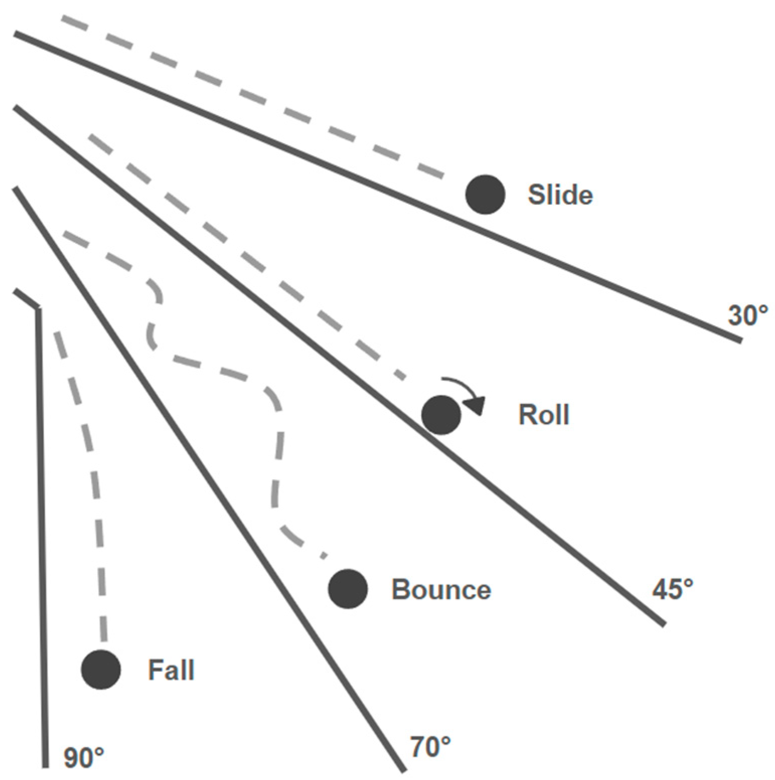
Concerning rockfall, when a rockfall boulder moves down a slope, it interacts with the terrain surface through four modes of motion, primarily depending on the angle of the slope (Figure 2). Listed from the steepest to flattest slope, these modes are freefall, bouncing, rolling, and sliding [6,7,8]. A boulder may experience one, multiple, or all of these modes before coming to rest.

The concept of tortuosity can be applied to describe the convoluted path that the rock takes while moving down the slope if the location of the rock is known for the entirety of its trajectory. Using a three-dimensional modeling software such as RocFall3, location coordinates from the fall can be exported, and the tortuosity can be calculated. Applying the concept of tortuosity to a rockfall path has not been recorded before in the literature.

In rockfall trajectory research, runout distance and lateral dispersion are often used to describe the predictability of multiple rockfall events from a single source location by quantifying the spread of fallen boulders [9]. Runout describes the straight-line distance from the seeder to the final location of a boulder. Dispersion is the minimum area required to encapsulate the seeder (or source) and final resting location of all boulders from a rockfall event (Figure 3). If a rockfall event consists of only a single boulder traveling down a slope, then there is no recorded dispersion, but there is a runout distance. Additionally, runout and dispersion only describe the final resting location of a boulder and do not provide any insight into the variable motion of the boulder during the fall. Together, tortuosity, dispersion, and runout distance can be used to fully analyze the trajectory and final location of fallen boulders to inform the design and placement of protective measures. This is an unexplored area of rockfall research.

To perform a tortuosity calculation, two pieces of information are required: the straight-line distance in three-dimensional space measured between the boulder’s original and final location, and the total path distance the boulder took while moving downslope. Tortuosity is calculated by dividing the total path length by the straight-line path length, as described in Equation (1). The minimum tortuosity value is one, meaning the boulder traveled in a perfectly linear path downslope.

$$Tortuosity={\displaystyle \frac{Total Path Length}{Straight Line Path Length}}$$

(1)

One current limitation of calculating rockfall tortuosity is that individual boulders lose contact with the ground during the motion modes of falling and bouncing. Rockfall modeling software (RocFall3 by Rocscience) records the location of a boulder at each point in a simulation. The location is associated with one of three descriptors: slope impact, contact, or projectile. However, these definitions are not clearly defined within the Rocscience software (version 5.007) documentation or the relevant literature, and it is unclear if the terms slope impact and contact differ. For this study, all three descriptors were considered for calculating tortuosity to provide the maximum information regarding the boulders position throughout the movement down slope.

2. Materials and Methods

2.1. Local Geology

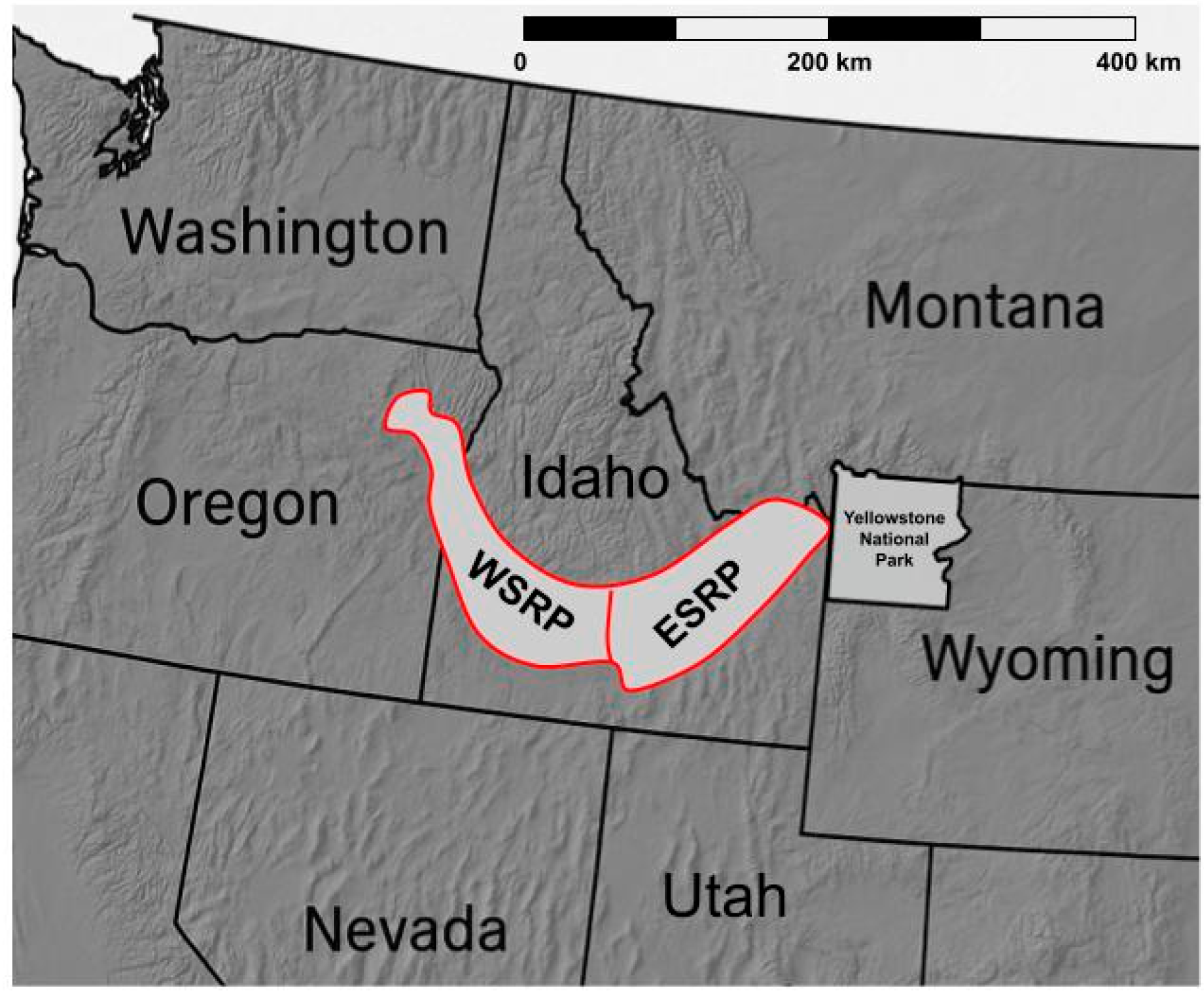
The study is located in Boise, ID, USA, within the western portion of the Snake River Plain (SRP). The SRP is a large, crescent-shaped geologic feature that stretches from the Idaho–Oregon border to Yellowstone National Park (Figure 4). It is home to eight of Idaho’s most populous cities and is a major agricultural area. The SRP is divided into its western and eastern constituents, WSRP and ESRP. The WSRP, where the site is located, is a southeast–northwest trending graben or topographic depression extending from the Idaho–Oregon border on the west to Twin Falls, Idaho on the east.

The graben structure was formed by downfaulting approximately 11 to 9 million years ago. The downfaulting created space for massive magma flows to occur, resulting in large basalt depositions [11]. It also generated space for water to accumulate, resulting in the formation of ancient Lake Idaho, which covered the WSRP from about 9 to 2.5 million years ago. During this time, lacustrine deposits from the lake covered much of the previously deposited basalt throughout southwest Idaho. The lake eventually overtopped a drainage divide near present-day Huntington, Oregon, and drained into what is now the lower Snake River [12].

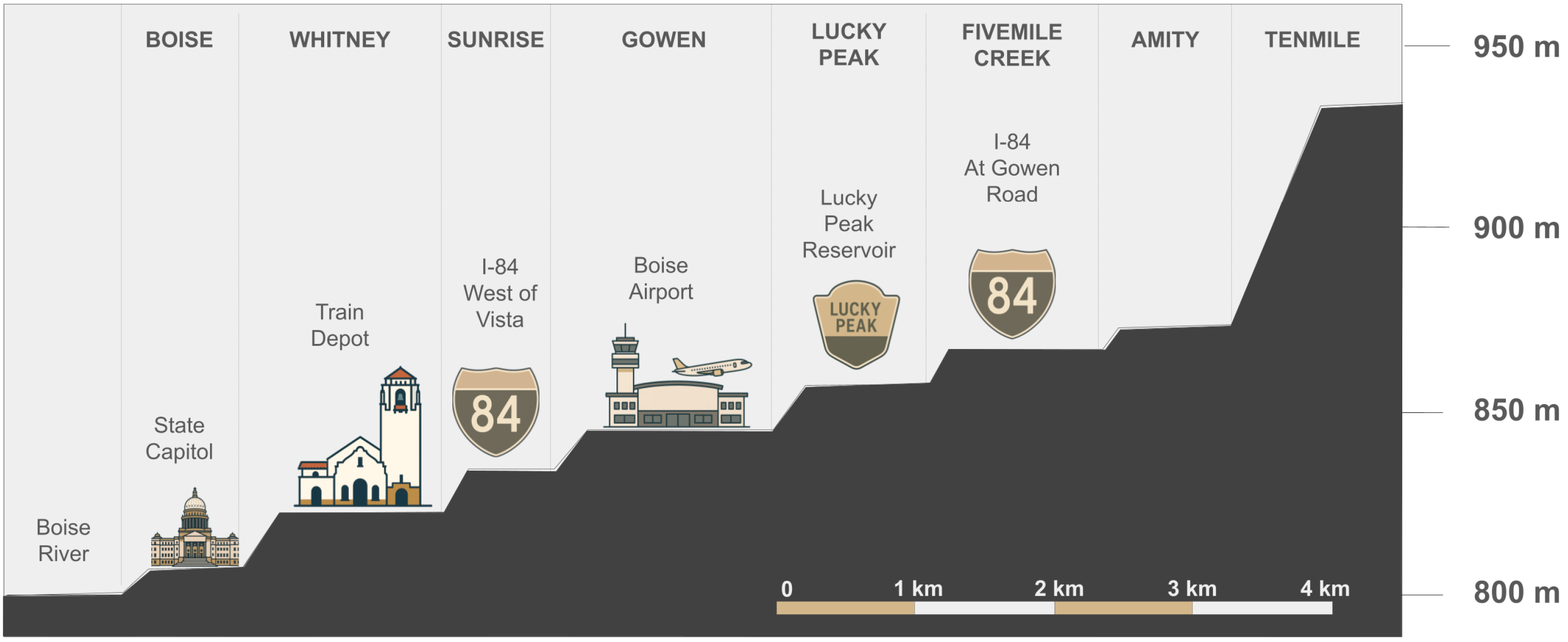
Over time, the Boise River, which is fed by snowmelt from the Sawtooth Mountains and empties into the Snake River, has downcut through the sediment deposited by Lake Idaho. After each downcutting event over the last 2 million years [13], the river further exposed the underlying basalt, resulting in eight distinct terraces in southeast Boise (Figure 5).

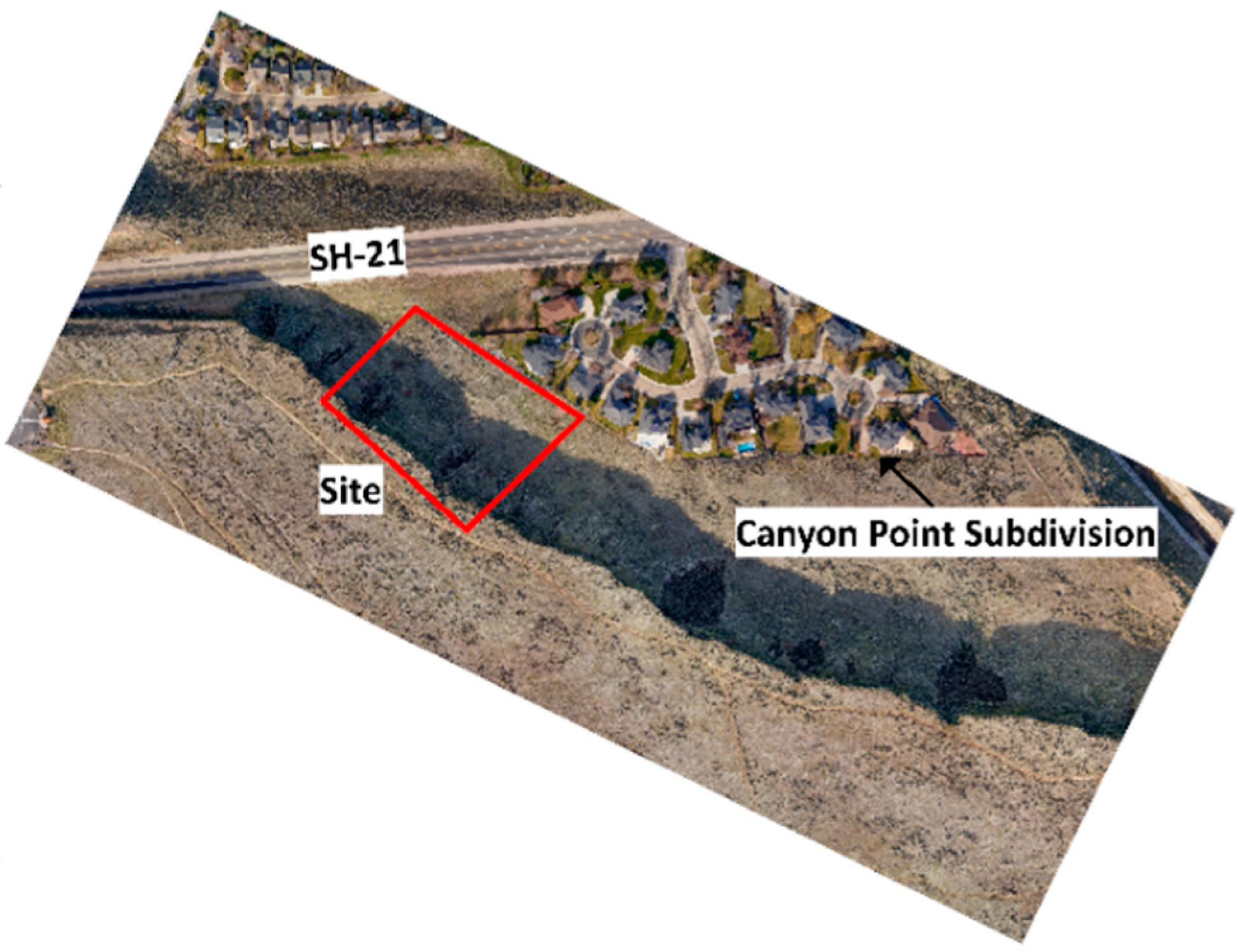
2.2. Study Site

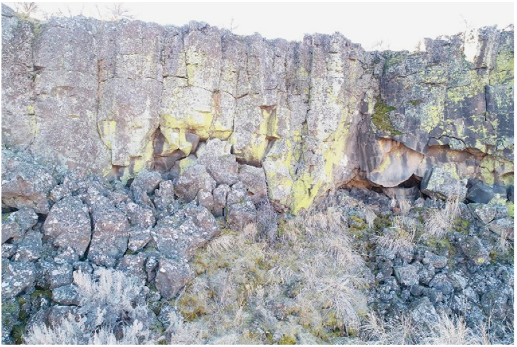
The study site for this research is part of the second terrace from the river, the Whitney Terrace (Figure 6). Along this terrace is a prominent columnar jointed basalt cliff featuring distinct vertical and horizontal discontinuities that divide the basalt into hexagonal-shaped blocks. The exposed basalt cliff face, shown in Figure 7, varies between five and seven meters in height.

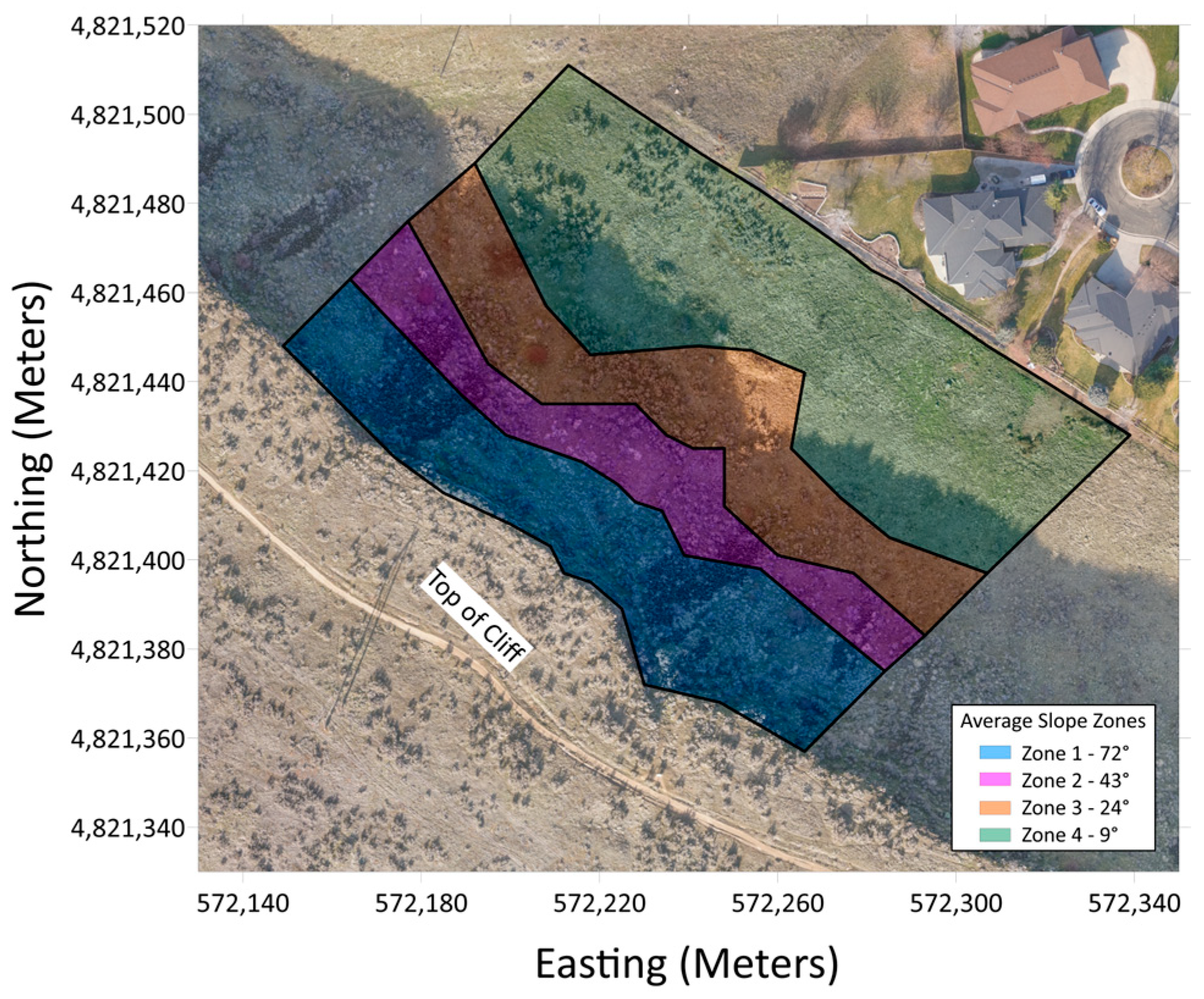
The slope beneath the cliff face is segmented with four distinct slopes, ranging from 72 degrees to 9 degrees, as shown in Figure 8. The site area is approximately 16,000 square meters (1.62 ha), and features deposited boulders, talus deposits, and sparse sagebrush vegetation.

2.3. Model Surface Generation

Five surface models were created for this site using a LiDAR-enabled UAV. In the field of rockfall trajectory research, there are three accepted ways to describe the resolution of a LiDAR-generated surface: number of points (pts), spatial resolution (m), and average point density (pts/m²). The number of points describes the total number of points obtained from a LiDAR scan. Spatial resolution describes the width of each pixel that comprises the digital elevation model (DEM) generated from the surveyed LiDAR point cloud [14,15]. A more convenient measure of resolution is the average point density, which describes the average number of points per square meter collected from a LiDAR scan [16,17].

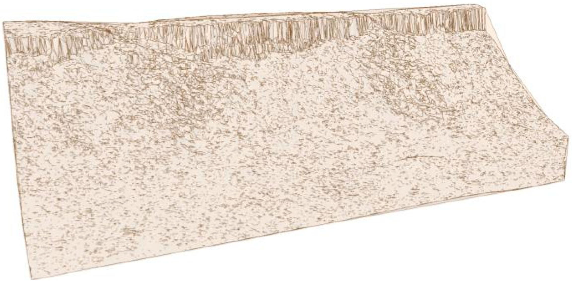
Although the initial resolution of our site-specific LiDAR survey was 291 pts/m² (186 million data points), RocFall3 software could not handle a point cloud this large. Hence, the point cloud was downsampled to generate the five model resolutions described in

Table 1. Terrain model resolutions.

Number of Points (pts)	Spatial Resolution (m)	Average Point Density (pts/m2)
100,000	4	6
150,000	3.27	9
300,000	2.31	19
900,000	1.34	56
1,200,000	1.16	74

and shown in Figure 9 and Figure 10. As a point of reference, publicly available LiDAR data collected by the Idaho LiDAR Consortium has an average point density of 13 pts/m². These publicly available LiDAR sources are often used as model inputs by design engineers and may lack the necessary detail to capture influential terrain features accurately.

2.4. Model Ground Properties

In addition to site geometry, ground properties, namely restitution and dynamic friction coefficients, are critical inputs to accurate rockfall trajectory modeling. A previous study conducted at the same site determined that a normal coefficient of restitution value of 0.3 and a dynamic friction value of 0.56 were most suitable. These values were determined by performing a two-dimensional calibration of the site using the locations of existing fallen boulders. For the calibration, the coefficients of restitution were systematically adjusted until the locations of the simulated boulders was within one-half of a standard deviation of the calibration (actual) boulders [18].

The study site was chosen to be modeled as homogeneous, meaning the same coefficients of restitution and dynamic friction values were applied to the entire surface. All the simulated boulders originated from the same seeder location with no initial velocity. This simulates boulders becoming detached from the cliff face, free-falling, and then tumbling down the slope.

2.5. Model Boulder Size

Based on field reconnaissance, four different boulder sizes and associated masses, categorized as small, medium, large, and extra-large, were modeled. Field observations indicated that a gamma distribution was most appropriate for describing the observed mass distribution for each boulder size.

Table 2. Simulated boulder mass properties.

Boulders	Minimum Mass (kg)	Mean Mass (kg)	Maximum Mass (kg)	Standard Deviation (kg)
Small	1.1	43.8	98.2	26.6
Medium	102.8	174.7	298.8	58.2
Large	300.6	431.0	596.2	96.2
Extra Large	601.4	2637.0	9366.7	2658.0

contains the minimum, mean, and maximum masses and the associated standard deviations used in the simulations.

2.6. Model Boulder Shape

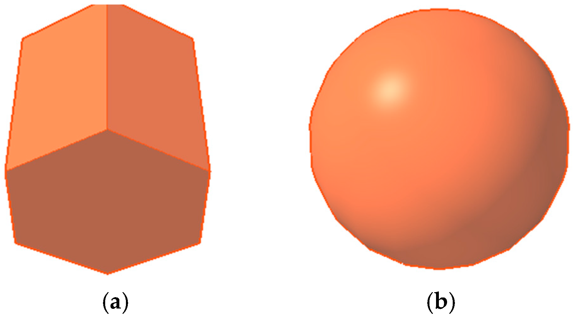
Two boulder shapes were chosen for the rockfall simulations. The first is the extruded polygon hexagon, a common shape for columnar jointed basalt [19] and similar to many of the boulders surveyed at the site. These will be referred to as hexagons. The other selected shape was a sphere. Although research has shown that spherical shapes often overestimate the runout distances of simulated boulders [20], they continue to be used as a common default rock shape for many rockfall simulation programs. Figure 11 depicts the hexagonal and spherical shapes from the RocFall3 software.

2.7. Rockfall Simulations

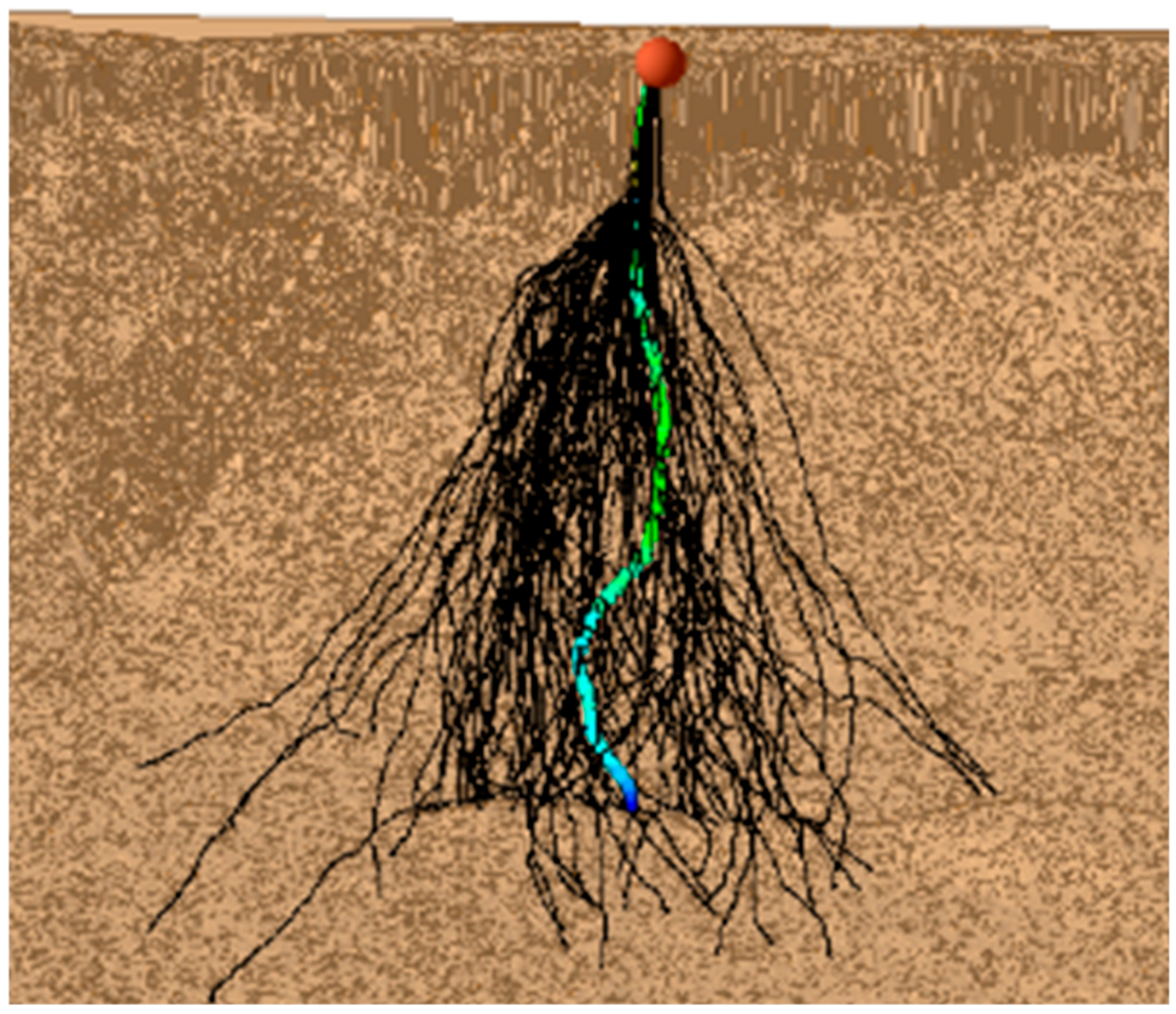
Forty rigid body simulations were performed using the five terrain models and four boulder sizes. Each simulation consisted of determining the trajectories of 500 individual boulders. In total, the trajectories of 20,000 boulders were simulated for this study. Figure 12 shows the simulated paths for 500 individual boulders. All boulders originated from the same source location (seeder) indicated by the large sphere. The boulder paths are not linear and the boulders follow a tortuous path down slope.

2.8. Data Analysis Approach

To assess the effect of terrain resolution, boulder mass, and boulder shape on tortuosity, the 20,000 output trajectory files from RocFall3 were analyzed using Python (version 3.13.3) and MATLAB (R2024b) scripts. These scripts automated the calculation of the total path length, straight line distance, and tortuosity.

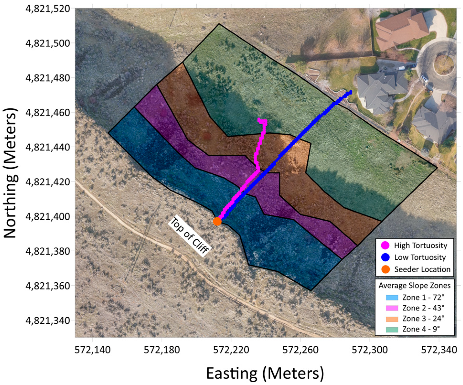
Figure 13 shows examples of high- and low-tortuosity boulder paths from simulations at the study site superimposed on an orthomosaic image showing the slope zones. The magenta path, showing a high tortuosity, is a relatively straight line as the boulder progresses downslope on the steepest part of the slope. As the slope angle decreases, the path deviates from a straight line, which increases the tortuosity values. The blue path, showing a low tortuosity, is a relatively straight-line path regardless of the slope angle.

2.9. Water Droplet Analyses

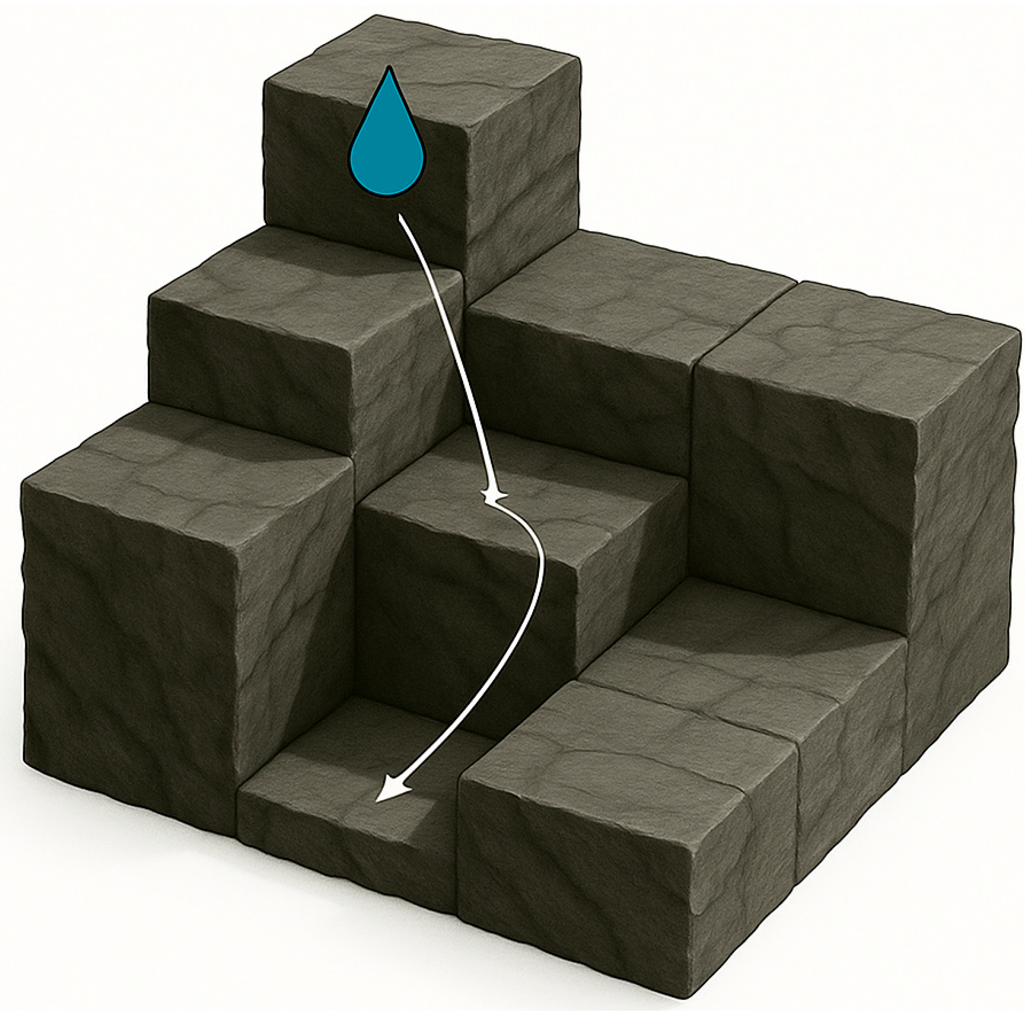
An ancillary water droplet analysis for the site was also performed. As previously discussed, tortuosity originates from hydraulic applications, and hydrologists often use water droplet analyses to trace the path of a droplet of water as it moves down an impervious slope to distinguish catchment areas and surface water basins [21,22]. As shown in Figure 14, the simulated droplets will follow the path of least resistance and stop where a level surface or localized depression is reached [23].

The concepts incorporated into a water droplet analysis are similar to those performed for a rockfall analysis. One key difference is that boulders in a rockfall analysis can move downslope by all four modes of motion (freefall, bounce, roll, and slide), while water droplets cannot experience bouncing. By only considering the low-energy rolling and sliding movements of boulders, the water droplet analyses and rockfall simulation were compared to see where boulders would congregate.

Civil 3D (by Autodesk) was used to perform the hydraulic analyses using the same five rockfall terrain models and the same seeder location. The output from the water droplet analysis was a three-dimensional polyline describing the droplet’s trajectory. Similarly to previous analyses, the coordinates associated with each polyline vertex could be used to compute the total path length and straight-line distance. From these two values, a tortuosity value was calculated.

For direct comparison, the rockfall modeling procedure in RocFall3 was modified to more closely resemble the water droplet analyses in Civil 3D. The first modification was modeling with a lumped mass approach rather than a rigid body approach. Lumped mass assumes the falling boulder to have no physical size and be modeled as a single point, just as a water droplet would be. Additionally, the mass of the boulder was set at 0 kg, matching the water droplet models computational approach.

3. Results and Discussion

3.1. Rockfall Results

Table 3. Tortuosity results for spherical boulders.

Terrain Resolution (pts/m2)	Mass	Average	Maximum	Minimum	Standard Deviation
6	Small	1.07	1.15	1.05	0.01
	Medium	1.07	1.13	1.05	0.01
	Large	1.06	1.10	1.05	0.01
	Extra Large	1.06	1.07	1.05	0.00
9	Small	1.08	1.22	1.05	0.01
	Medium	1.07	1.12	1.05	0.01
	Large	1.06	1.14	1.05	0.01
	Extra Large	1.06	1.07	1.05	0.00
19	Small	1.08	1.40	1.05	0.03
	Medium	1.08	1.29	1.05	0.02
	Large	1.07	1.26	1.05	0.02
	Extra Large	1.06	1.11	1.05	0.01
56	Small	1.16	1.40	1.06	0.08
	Medium	1.13	1.40	1.06	0.07
	Large	1.13	1.40	1.05	0.07
	Extra Large	1.08	2.08	1.05	0.06
74	Small	1.14	1.58	1.05	0.08
	Medium	1.13	1.47	1.05	0.07
	Large	1.13	1.36	1.05	0.06
	Extra Large	1.08	1.86	1.05	0.06

and

Table 4. Tortuosity results for hexagon boulders.

Terrain Resolution (pts/m2)	Mass	Average	Maximum	Minimum	Standard Deviation
6	Small	1.07	1.19	1.05	0.01
	Medium	1.07	1.13	1.05	0.01
	Large	1.07	1.15	1.05	0.01
	Extra Large	1.08	1.23	1.05	0.02
9	Small	1.07	1.14	1.05	0.01
	Medium	1.07	1.15	1.05	0.01
	Large	1.07	1.18	1.05	0.02
	Extra Large	1.08	1.16	1.05	0.02
19	Small	1.07	1.14	1.05	0.01
	Medium	1.08	1.15	1.05	0.01
	Large	1.08	1.16	1.05	0.02
	Extra Large	1.08	1.18	1.06	0.02
56	Small	1.09	1.28	1.05	0.03
	Medium	1.09	1.34	1.04	0.04
	Large	1.09	1.47	1.06	0.03
	Extra Large	1.09	1.18	1.06	0.02
74	Small	1.09	1.24	1.06	0.03
	Medium	1.10	1.37	1.06	0.04
	Large	1.08	1.79	1.04	0.04
	Extra Large	1.09	1.23	1.06	0.02

contain the rockfall tortuosity results for the spherical and hexagonal shapes, respectively. The results include the minimum, average, and maximum tortuosity values and the standard deviation for each of the 40 simulations.

Several general comments can be made from the data in Table 3 and Table 4 and Figure 15 below. Overall, the simulations show that spheres have larger tortuosity values than hexagons. For spheres, tortuosity increases slightly with size and increases with terrain resolution. For hexagons, tortuosity remains approximately constant with size and minimally increases with increasing resolution. These general findings are further investigated below.

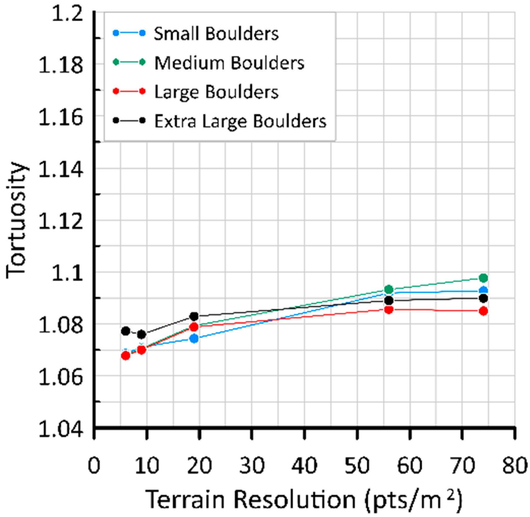
3.2. Tortuosity of Spherical Boulders

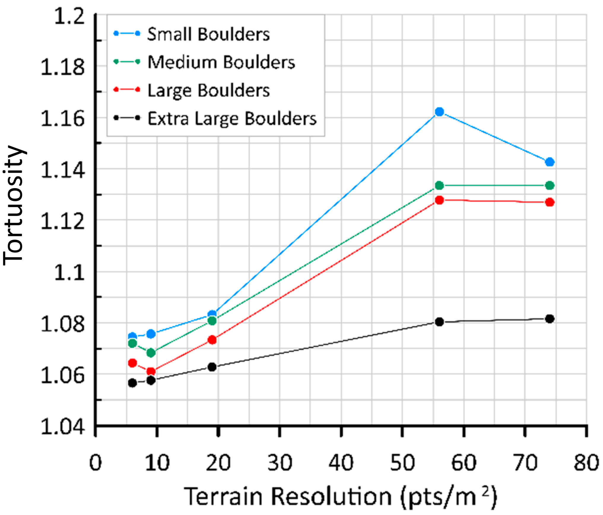
The effect of terrain resolution on the tortuosity of spherical boulders is shown in Figure 16 below. All average tortuosity values for spheres were between 1.06 and 1.16.

For spherical boulders, smaller boulders consistently experienced larger tortuosity values than larger boulders. This is because larger boulders have more momentum due to their increased mass and are less likely to be impacted by terrain features.

As terrain resolution increases, the effect of boulder size is also more prominent. This is expressed in Figure 16, where the gap between each line increases with resolution. This can be attributed to a higher presence of asperities, which smaller boulders are still more likely to be influenced by.

Additionally, as terrain resolution increases, average tortuosity also increases, until reaching a threshold at 56 pts/m². After this point, tortuosity remains constant or decreases. This is likely because at low resolutions, asperities in the ground surface are not yet revealed, and cannot alter the boulder’s trajectory. As the resolution increases, these asperities become more present, until there are so many that they begin to confine the motion of the boulder, preventing substantial trajectorial deviation.

3.3. Tortuosity in Hexagonal Boulders

The effect of terrain resolution on tortuosity for hexagonal boulders is shown in Figure 17 below. All average tortuosity values for hexagons were between 1.07 and 1.10, a much tighter spread than the spherical boulders.

For hexagonal boulders, smaller boulders do not consistently experience larger tortuosity values than larger boulders. Additionally, the range between boulder sizes is relatively small, both of which are in contrast to observations of spherical boulders.

As terrain resolution increases, the average tortuosity does increase, but the effect of boulder size does not appear to change. These discrepancies between the results of spherical and hexagonal boulders imply that the boulder’s angularity plays a crucial role in tortuosity and rockfall trajectory in general.

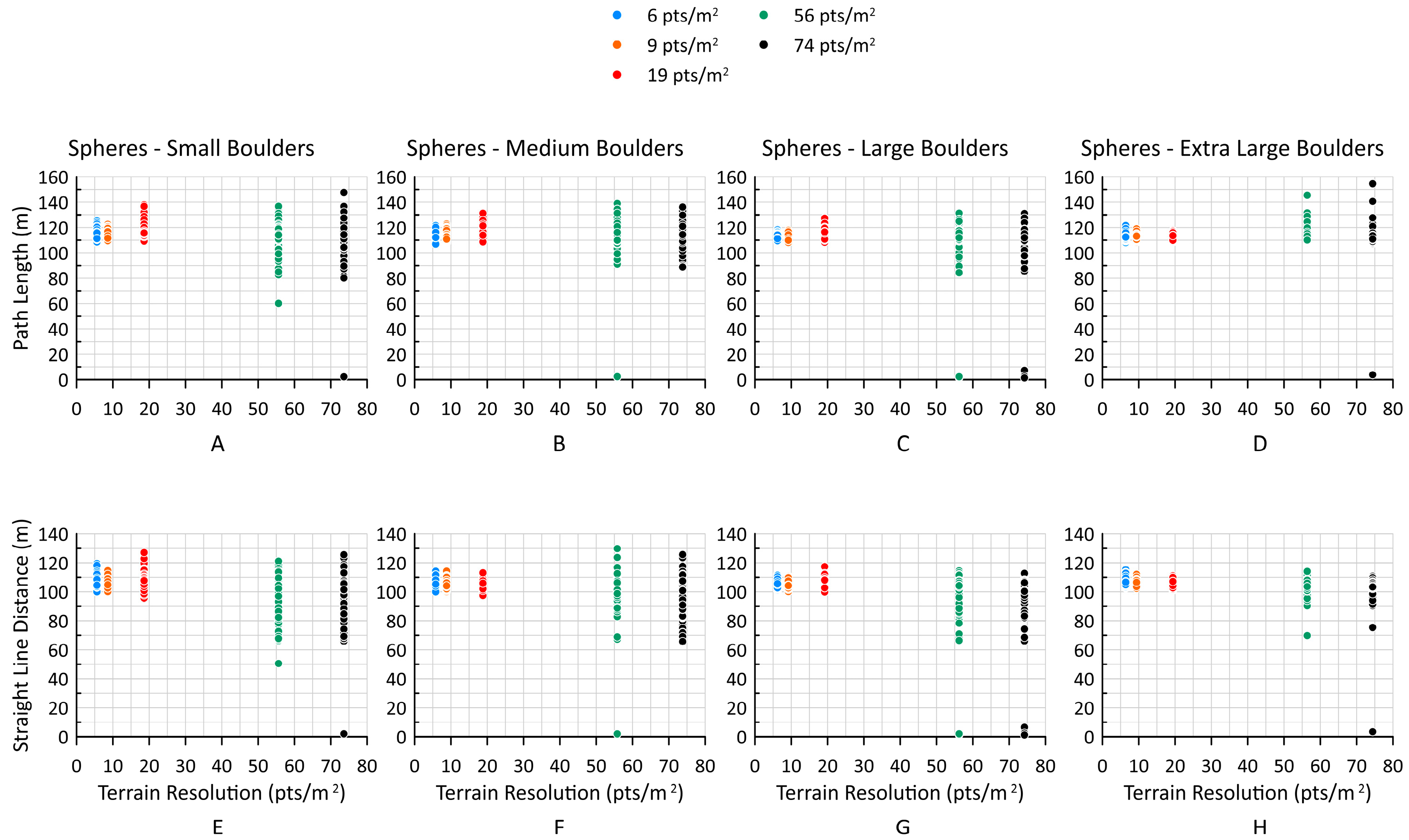
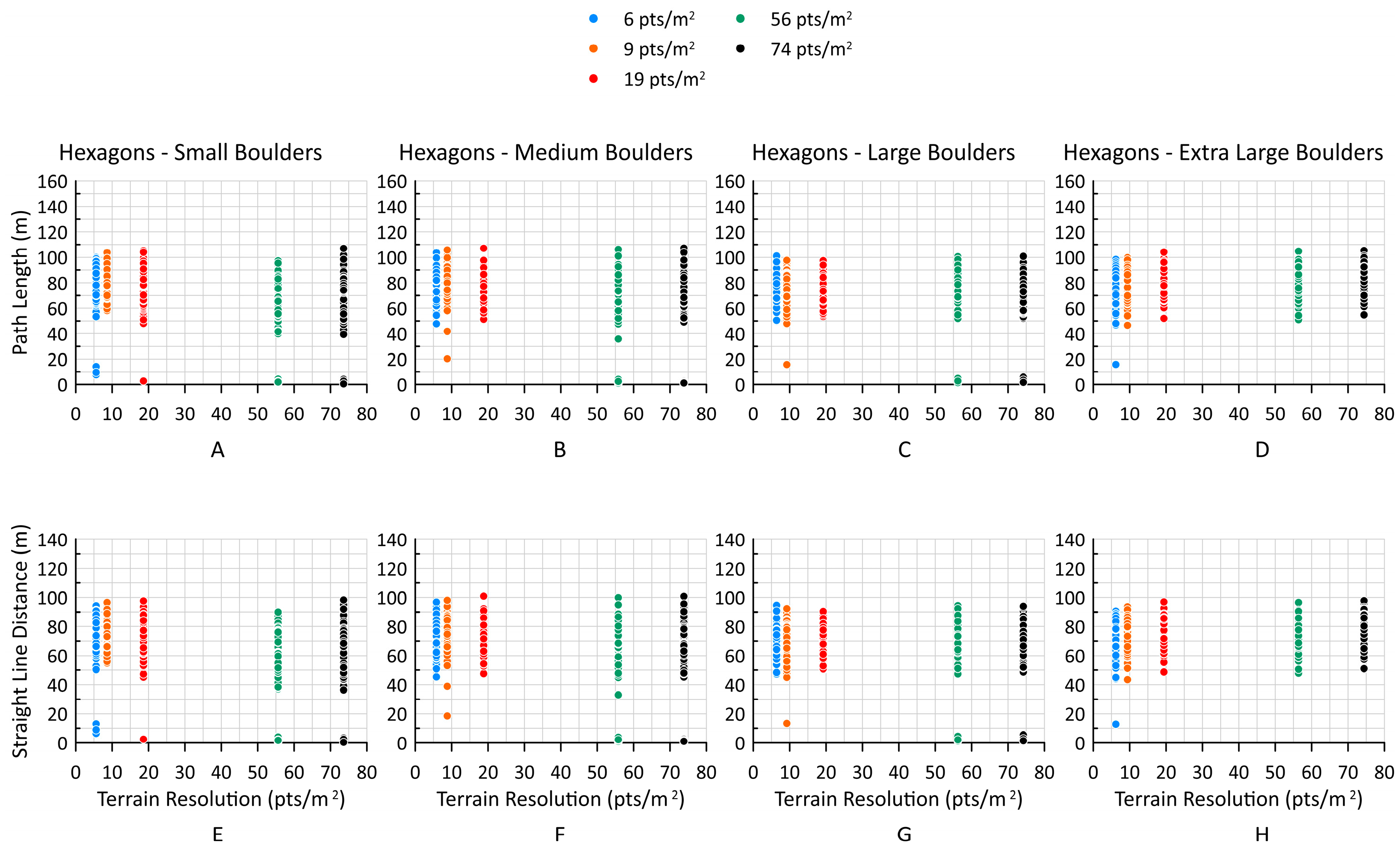
3.4. Components of Tortuosity

Because tortuosity is the ratio of path length to straight line distance, a change in either of these components proportionally affects tortuosity. To further understand tortuosity variability, the two components were plotted separately for all simulations, as shown in Figure 18 and Figure 19.

The path length and straight-line distance values are very similar across all sizes and resolutions for the hexagonal boulders. The path length and straight-line distance values are more variable for spherical boulders. Across all boulder sizes, the path lengths and straight-line distances fall in a very narrow range for the 6 and 9 pts/m² resolutions, with the range becoming smaller as the spherical boulder size increases. At a terrain resolution of 19 pts/m², the range of path length and straight-line distance values becomes larger, except for the extra-large spherical boulders, where it becomes smaller. At the highest resolutions, the path lengths and straight-line distances have the largest range of values. The range of values is similar for small through large spherical boulders, but the range of values decreases for the extra-large spherical boulders.

It was hypothesized that the change in tortuosity could be attributed to a distinct change in either path length or straight-line distance. However, the data presented in Figure 18 and Figure 19 show that both components of tortuosity are affected by terrain model resolution for the spherical and hexagonal boulders.

3.5. Water Droplet Analysis

Compared to the previous rockfall models, the hydraulic analyses show a substantial decrease in distance traveled, whether for the straight line or total path length (

Table 5. Water droplet analysis results.

	Civil 3D			RocFall3
Terrain Resolution (pts/m2)	Total Path Length (m)	Straight Line Distance (m)	Tortuosity	Total Path Length (m)	Straight Line Distance (m)	Tortuosity
6	57.51	53.84	1.07	58.61	54.87	1.07
9	65.48	60.64	1.08	61.70	57.39	1.08
19	19.40	16.20	1.20	60.83	60.19	1.01
56	5.94	5.86	1.01	0.87	0.54	1.63
74	6.79	6.23	1.09	51.12	46.58	1.10

). The Civil 3D models show what we would expect to be true in a hydraulic analysis, as the terrain resolution increases, more asperities become present, increasing the likelihood of a level surface or localized depression at any given point. This roughness increase results in an overall path length decrease. The straight-line distance shows the same general trend. In contrast, the RocFall3 results show consistent total and straight-line path lengths except for the second highest terrain resolution. This value appears to be an outlier in the data. The contrast between the two can be attributed to the different computational approaches between Civil 3D and RocFall3. More specifically, Civil 3D is strictly elevation-based and does not consider momentum. This leads to particles being more affected by small terrain features.

One key observation is that at very short path lengths, tortuosity tends to be an unreliable measure of rockfall trajectorial variability. This is because with a very small denominator in the tortuosity equation, a small change in the numerator can have significant implications. This is clearly observed in the 56 pts/m² resolution RocFall3 modeling, where tortuosity reached a value of 1.63 with a path length of less than 1 m. It is intuitively obvious that a boulder traveling less than 1 m does not provide a wide range of uncertainty in where it will end up, but the tortuosity value does not reflect this. This highlights the critical role of using both tortuosity and dispersion areas to describe rockfall predictability.

Another important observation is the role of bouncing in tortuosity. The hydraulic analyses removed bouncing, the highest energy mode of motion. It was expected that bouncing was a primary contributor to tortuosity, and that by removing it, the boulder path would be less variable. However, the opposite was observed. Hydraulic analyses showed an increased average and range in tortuosity values. It is concluded that this can be attributed to the role of momentum in motion predictability. Rocks that have very high kinetic energy also have high momentum and are less likely to be affected by terrain features. Boulders with high kinetic energy tend to follow straight line paths, meaning they are more predictable and their paths have lower tortuosity. Additionally, objects in projectile motion experience a fully understood and predictable parabolic trajectory, removing the possibility of path alteration while in the air. By excluding this in the hydraulic analysis, the opportunity for variability was reduced and a decrease in tortuosity was observed.

4. Conclusions

The tortuosity of the boulders paths was calculated using the ratio of the total path distance of the boulders to the straight-line distance from the seeder location to the final resting location. For both shapes, as the terrain resolution increased, the tortuosity values increased. This is likely because as the terrain models became more defined, the number of terrain features increased, which would deviate boulders from their straight-line paths. The boulder shape also influences tortuosity values, as spheres had larger values when compared to hexagons. Regarding boulder masses, as the mass increased for spherical boulders, the tortuosity values decreased. This is likely because as the spheres became larger, it would take a more significant terrain feature to alter their straight-line path down the slope. No consistent trend was established between boulder mass and tortuosity for hexagonal boulders. However, the hexagonal boulders followed a more constrained path on this rough terrain, demonstrating different results than previous research on smooth surfaces [24,25], highlighting the role of slope roughness.

The components of tortuosity, the total path length, and the straight-line distance were analyzed to determine if one component impacted the tortuosity value more than the other. It was found that both of these components equally impact the tortuosity values for spherical and hexagonal boulders.

A water droplet analysis was also performed to assess how tortuosity varied with the four modes of motion and their associated kinetic energies. By eliminating the high-energy mode of bouncing, the water droplet analysis highlighted the constraining role that bouncing has in the trajectory. By removing it, tortuosity increased in both quantity and variability.

Three key findings can be extracted from this study, implementable by both researchers and rock slope assessment engineers:

• Publicly available LiDAR is often not collected at a high enough resolution to accurately model rockfall. This study demonstrates that terrain resolution directly and substantially impacts the trajectories of boulders, necessitating higher resolution site-specific LiDAR mapping of rockfall sites.
• The mass and shape of simulated boulders play a large role in rockfall dynamics and trajectories. When performing a rockfall study, it is imperative that the correct boulder size and shape are modeled based on observations and measurements made during field reconnaissance activities.
• Tortuosity is a useful measure in understanding the variability of rockfall boulder path downslope, but it does not replace the traditional measure of dispersion. The two measures should be used together to describe the path the boulders took and their final resting locations.