1. Introduction
In recent years, numerous applications of data-driven approaches have been successfully implemented across various civil engineering fields, including geoengineering [
1]. Driven by the need to address the challenges of modern construction projects [
2], the field has adopted the integration of digital tools, automation, and advanced analytical techniques, all of which dramatically increase productivity and accuracy in decision-making [
3].
MWD technology is an important component of modern tunneling projects, including drill-and-blast tunneling, and is a prime example of the successful integration of advanced tools and digitalization [
4]. This technology allows real-time data collection during drilling operations. An analysis of collected MWD data can enable an assessment of the condition of the rock mass, prediction of potential hazards, assurances of the tunnel’s structural integrity [
5], and, in general, can help to support informed decision-making that is aligned with the encountered geological conditions [
6].
While MWD data have the potential to provide insights into drilling conditions and the properties of the rock mass, its direct application in predictive modeling is subject to some limitations. Sensor inaccuracies, mechanical calibration errors, and fluctuations in drilling parameters introduce inconsistencies, making direct interpretation unreliable. Variability in geological formations further complicates direct MWD-based assessments, as similar drilling responses may correspond to different rock types under varying conditions.
Another challenge is the high degree of redundancy and noise in MWD datasets. Certain parameters exhibit strong intercorrelations, while others provide minimal additional predictive value. The presence of outliers—caused by sudden changes in drilling conditions or sensor anomalies—necessitates rigorous pre-processing to prevent misleading conclusions. With such limitations in data quality, traditional predictive models relying solely on MWD may struggle to deliver accurate predictions or extract meaningful patterns from the MWD data.
While common approaches to data pre-processing, including MWD data, often rely on normalization, statistical aggregation (mean, min, and max), or handcrafted features, they frequently fail to capture localized dependencies between variables that change over the borehole depth. Our method addresses this gap by using correlation coefficients derived from sliding windows across the MWD time series. This strategy captures dynamic relationships between drilling parameters and transforms them into statistically stable features, enhancing model robustness and consequently preserving the physical interactions encoded in raw data.
To address the challenges of MWD data analysis, researchers employ machine learning (ML)-based approaches to enhance the interpretability of MWD data and improve the robustness of geotechnical analysis. As a branch of artificial intelligence, ML is used to extract patterns from data, enabling more accurate and data-driven predictions [
7]. The application of ML to MWD data is a relatively new field but has already shown great potential [
8]. ML-based predictive models outperform traditional mathematical approaches in accuracy and computational speed [
9] and have been successfully applied to different aspects of blasting operations [
6,
10].
However, there is room for improvement in the accuracy of ML models trained on MWD data. Research from A. Shahri et al. [
11] highlights how the complexity of handling large-scale MWD data due to, e.g., multiform stacking, imposes challenges in extracting accurate geoengineering interpretations. As a solution, the authors suggested normalizing and filtering out noisy data to ensure more accurate results from ML models predicting rock quality conditions. It is known that data quality is the most critical factor influencing the accuracy of outputs from the MWD data analysis and that data preparation and pre-processing steps are extremely important in creating a good training dataset for ML models [
12].
In this work, we continued the research reported in [
13] and further investigated how the preparation and pre-processing of MWD data contribute to the successful application of ML for predictive analysis and decision-making. The primary task of an ML model is to predict the volume of explosives needed to avoid over/underbreaks, using MWD data as inputs. This study focuses on identifying pre-processing and feature engineering techniques that optimize the construction of a training dataset, enabling the ML model to effectively uncover hidden patterns in MWD data. The goal is to develop pre-processing strategies that preserve and enhance the informational content of the dataset, ensuring that ML models trained on it achieve the highest possible predictive accuracy. To achieve this, we propose a pre-processing method based on correlation analysis that is designed to amplify meaningful relationships within MWD data while reducing noise and redundancy. By applying this approach, the dataset is transformed into statistically optimized features, enhancing the predictive accuracy of ML models, as demonstrated in
Section 4.2. The results confirm that pre-processing significantly improves the reliability of ML-driven geotechnical assessments by extracting robust patterns that are not apparent in raw MWD data.
This research also seeks to bridge the gap between data collection and utilization, demonstrating a methodical way to select datasets for machine learning beyond a trial-and-error approach [
8].
2. Data Preparation
When preparing the training data, one aims to build representations of the data that improve the identification of underlying patterns during ML model training. The preparation process can be separated into three steps: data cleaning, normalization, and feature engineering.
Data cleaning: during drilling, MWD systems continuously record several parameters. These data are stored as instrumental logs of the real-time interaction between the drilling machinery and the rock mass in a plain text format. The cleaning of MWD data aims to handle logs of drilling data and related information to extract information required for data-driven modeling. First, all collected MWD logs shall be converted to a tabular (structured) form. Then, tables of “raw” MWD data shall be cleansed: this includes procedures such as noise removal, outlier detection, missing values handling, and correcting any inconsistencies. Data cleansing is crucial to ensure that the ML models are not “misled” by erroneous data, statistical biases, or other inaccuracies. Following cleansing, data integration is performed. This involves combining subsets of data into a single dataset or database to provide a comprehensive view of the process—in this case, tunneling operations. In this work, the authors, in addition to MWD data, also used operational records such as explosives data, tunnel geometry, and planned excavation data, all of which must be integrated into a single dataset. Proper data integration requires an alignment of these (differently) structured data into a unified table, where the impact of each parameter on the others can be examined. The integration process also includes checking data timelines, consistency, and completeness.
Normalization: the data normalization procedure ensures that the ML model remains unbiased due to differences in the scale of the data [
14]. Since the effectiveness of a normalization technique depends on the distribution of raw data, we first analyzed the statistical properties of MWD variables. The results showed that most features exhibited values within consistent, bounded ranges without extreme outliers, making min–max scaling a suitable choice. The min–max scaling method preserves the relative spacing between values while transforming all features into a fixed [0,1] range. This is particularly beneficial for ML models that are sensitive to input magnitude differences, such as neural networks and tree-based models, where maintaining proportionality enhances learning stability and efficiency. Alternative normalization techniques, standardization (Z-score normalization), and robust scaling were also considered. A detailed discussion of the scaler selection procedure is provided in
Section 3.
Feature engineering: during this step, a selection of a subset of relevant variables (or the creation of new ones) shall be made. The selection of variables (features) is based on domain knowledge or statistical analysis results. For instance, the rotational speed ratio to thrust might be considered a proxy for hardware wear. The feature engineering step aims to develop a training dataset that enhances the ML models’ ability to detect complex patterns and relationships by providing a clearer signal to the predictive model.
Correlation analysis, a statistical tool that helps quantify the relationships between variables, can reinforce the normalization and feature engineering steps [
15]. When applied to MWD data, it allows for the correlation of the impact of rock mass conditions with MWD recordings. Therefore, it provides insights into the physics of rock mass drilling, which can guide future data collection and feature engineering efforts.
To construct the DDF dataset, Pearson correlation coefficients were computed for each pair of MWD parameters within sliding windows. This choice enables capturing the short-term, local dependencies between variables. The resulting set of coefficients represents how pairs of drilling variables co-vary during each drilling event. For example, a highly positive correlation between feed pressure and rotation speed within a window may indicate a stable drilling regime, while a low or negative correlation may signal irregularities in rock conditions.
In the next section, we will describe the foundational aspects of assessing the quality of a dataset for ML model training and demonstrate how using correlation coefficients together with the MWD data or alone is advantageous for this purpose.
3. Dataset Quality Assessment
Several metrics can be used to assess the informational content of datasets for ML training: entropy, statistical noise, normalized variance, dimensionality, and average correlation [
16]. Each metric measures the specific characteristics of the quality of the information in a dataset [
17]. When the goal is to choose the most “informative” dataset suitable for ML model training, a combination of these metrics shall be used. In the section below, we review the characteristics of each metric used in this work for the dataset assessment.
In ML, informational diversity within a dataset is important to improve the model’s ability to generalize to unseen data, reduce bias, and enhance predictive accuracy. Diverse information allows the ML model to train on a wide range of conditions, scenarios, or classes, enabling it to learn patterns that are broadly applicable rather than overfitting to specific, over-represented features. This promotes robustness through comprehensive feature learning when meaningful relationships across variables are captured. Overall, an ML model trained on datasets with high informational diversity will output more accurate and reliable predictions. The informational diversity can be described by entropy (H), a concept “borrowed” from information theory that quantifies the amount of information or uncertainty within a dataset. For a discrete random variable X with possible values {x
1, x
2, …, x
n} and probability function P(X), entropy is defined as:
where b is the base of the logarithm, typically 2, making the unit of entropy bits. A higher entropy implies greater randomness and potentially more information content [
18].
A high entropy means that the dataset contains diverse information, but this information must be balanced against the risk of having too much noise. Measuring noise content in a dataset is complex because noise can take many forms and is not always straightforwardly quantified. However, statistical noise estimation and data quality analysis are general methods and considerations for estimating noise in a dataset [
19].
In this work, we calculated the variance of residuals and the signal-to-noise ratio to estimate the statistical noise.
The variance of residuals—the divergence between observed values y and predicted values ŷ—serves as a noise indicator in a well-fitted model [
20]. The variance of residuals σ
2residuals can be expressed as:
where N is the number of observations.
A high residual variance indicates considerable noise, which could overshadow the signal. Originating from signal processing, the signal-to-noise ratio (SNR) determines the strength of the signal, or the desired pattern, against background noise. It is defined as:
A higher SNR means a more apparent distinction between the signal and the noise, indicating less noise content in the data [
21]. Although the interpretation of a statistical noise value shall be based on a general understanding of the dataset’s context and the objectives of ML modeling, there is a general guideline [
22] stating that high residuals and low SNR variance likely indicate poor data quality or collection issues, which could compromise ML model performance.
Since the variance in a dataset defines a spread of data points, normalization of the variance is essential, especially when comparing datasets with features on different scales. Normalized variance brings all features to a unified scale, preventing features with larger numerical ranges from dominating the variance calculation. The formula for variance (σ
2) is:
where x
i represents the data points, μ is the mean, and N is the number of data points.
While data normalization is important to ensure that different features contribute equally to the ML model, the choice of the specific scaling technique depends on the dataset’s characteristics, including the presence of outliers and the distribution of features. In datasets with widely varying feature ranges, improper scaling can lead to poor model performance, as certain features may dominate the learning process while others become negligible. Therefore, a comparative evaluation of different scaling methods is needed to determine the most suitable approach for pre-processing the dataset before ML training.
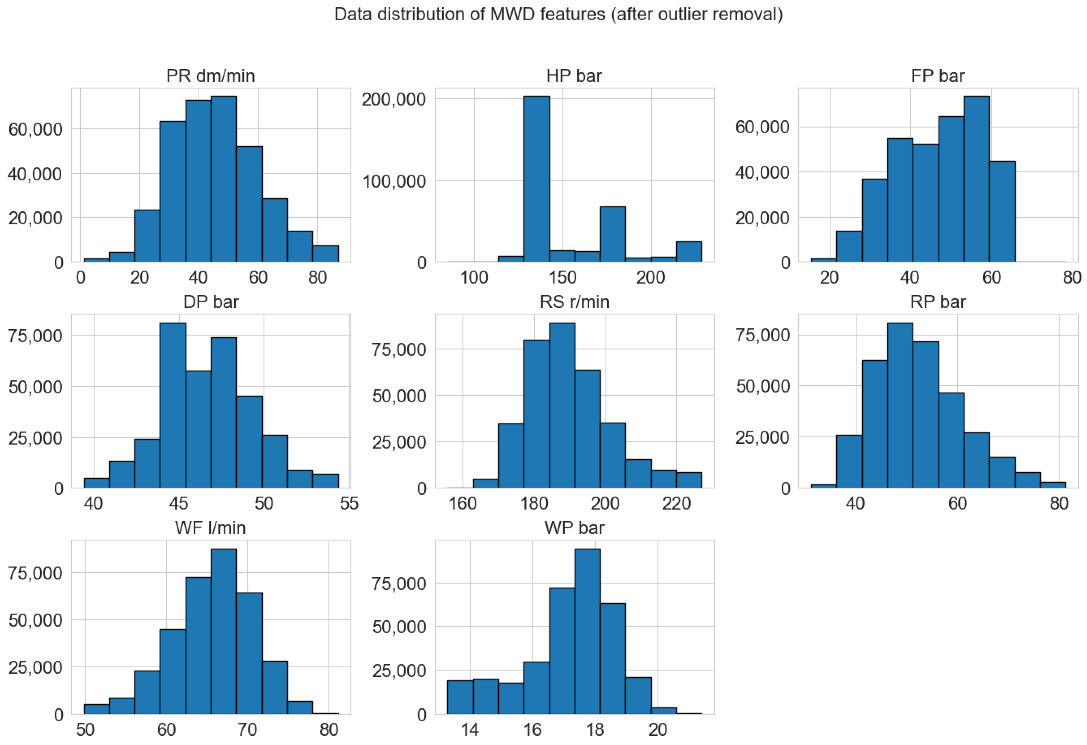
At first, the data distribution for each feature was analyzed (
Figure 1). While most MWD variables exhibit a normal-like distribution, the hammer pressure (HP bar) and the water flow (WF l/min) exhibit extreme values and, together with the forward pressure (FP bar) variable, display a skewed distribution of data values.
To ensure that the data normalization technique effectively preserves key statistical properties while minimizing distortions, we conducted a comparative analysis of three commonly used feature scaling methods: min–max scaling, standardization (Z-score normalization), and robust scaling. The goal of this comparison was to evaluate their impact on feature distributions and outliers in the dataset. The comparison was performed by scaling the DF dataset. Each scaler was applied separately, and the transformed data were analyzed using a statistical summary comparison and outlier sensitivity parameters.
For the statistical summary comparison, descriptive statistics, including the mean, standard deviation, minimum, maximum, and interquartile range (IQR), were computed before and after scaling. This summary shall highlight how each scaling method affects data spread, central tendency, and variability. For outlier sensitivity, we examined how each scaler handles the extreme values present in DF.
Comparing the results of the min–max scaling, standardization, and robust scaling methods, we observed that each method has distinct effects on feature distributions and statistical properties. Min–max scaling maintains the relative spacing between values while scaling the values to fit the range [0,1], but its sensitivity to outliers pushes the extreme values of the data into a compressed middle range. The interquartile range (IQR) of 0.08 for the min–max scaler is smaller than the IQR observed in standardization (0.12) and robust scaling (0.16). This reduction may affect the accuracy of the ML models as they rely on variations in absolute magnitude. The standardization (Z-score scaling) method, which transforms the dataset so that it has a mean of approximately 0 and a standard deviation of 1, can allow better maintenance of feature variability in a dataset and ensure a normal-like distribution of the data after transformation. However, the presence of extreme values in the DF resulted in some features having unusually large maximum values, such as a max of 39.46 for the “DP bar” variable. This suggests that the standardization method is not the optimal choice as, after its application, the data distribution remained shifted. Robust scaling, which scales features based on the median and interquartile range, proved to be the most resistant to extreme values. An IQR of 1.00, combined with a lower sensitivity to extreme values, demonstrates that this technique successfully reduces the influence of outliers while preserving key statistical relationships. Unlike min–max scaling, it does not force all values into a strict [0,1] range, and unlike standardization, it does not let outliers dominate the transformation.
Next, the outlier sensitivity test was carried out to confirm the impact of each scaler on extreme values. Min–max scaling compressed most values into a small range, therefore stretching the influence of extreme values to [0,1] and making it unsuitable for datasets with a high degree of outliers. Standardization, while normalizing variance, allowed outliers to create extreme deviations. Robust scaling, on the other hand, seems to be effective in reducing the influence of outliers by scaling based on percentiles instead of the mean and standard deviation. Given these observations, robust scaling can be selected as the most effective method in terms of outlier resistance.
Nevertheless, min–max scaling was ultimately applied in this study to ensure compatibility with transformer-based models, which require input features within a normalized [0,1] range. These models are sensitive to absolute value ranges during training, and unscaled inputs may hinder convergence and generalization. Thus, for this study, all numerical features were scaled using the min–max scaler.
A dataset’s dimensionality refers to the number of features or variables it contains. Higher dimensionality can lead to the “curse of dimensionality”, where the feature space becomes so large that the available data become sparse, causing an overfitting problem during ML model training.
The average correlation among features indicates the presence of linear relationships. MLMs might struggle to distinguish between features in datasets with high multicollinearity (highly correlated features), leading to unstable results [
23]. Usually, the average correlation among features is calculated as the average of absolute values of correlation coefficients between different pairs of features.
Training ML models on the best data is one of the most important conditions for ensuring the accuracy of the outputs. Applying the abovementioned metrics allows this selection to happen without a trial-and-error loop.
4. Results and Discussion
4.1. Choosing the Datasets
For this work, MWD logs generated by the drilling equipment (an Epiroc Boomer) were acquired and stored for analysis. Initially, a data cleaning routine, as outlined in
Section 2, was applied to the raw MWD data, which were provided as semi-structured text files. Ten drilling variables were identified and utilized throughout this work: borehole length, drilling duration, penetration rate, hammering pressure, feed pressure, dumper pressure, rotation speed, rotation pressure, water flow, and water pressure. The value of an over-excavated volume for each borehole was then integrated with MWD data.
For our study, three datasets were considered:
the original dataset (DF) was created from the cleaned and normalized MWD data;
the statistical dataset (SDF) was made from the pre-processed and normalized statistical values (per borehole min, max, and mean values calculated for every variable) of MWD data;
the derived dataset (DDF) was made from the correlation coefficients of MWD data, computed for every borehole using sliding window intervals.
To decide which dataset is more valuable for ML model training, we first conducted a correlation analysis among DF, SDF, and DDF features to assess the impact of data transformations on relationships between variables. DF has the highest correlation coefficient. As shown in
Table 1, DF contains five times more instances that can be attributed as outliers compared to SDF. These spikes of values in DF can be attributed to the normal variability of sensor readings during the drilling process. Since extreme values often amplify correlation coefficients, noise reduction was applied in SDF using statistical summaries, leading to lower correlation strengths. DDF has the lowest correlation coefficient. By computing the correlation coefficients for every borehole, we were able to obtain detailed information on the localized interactions between variables for each borehole. Unlike SDF, which replaces continuous values with single summary statistics, DDF retains a dynamic representation of drilling parameter relationships. Furthermore, by computing correlations over multiple windows instead of using individual point values, short-term fluctuations were further smoothed out in DDF, and only consistent, underlying dependencies between variables were kept.
Next, we assessed the dataset’s relevance by running a feature importance analysis using the random forest regressor (RFR) method. Feature importance analysis quantitatively measures each feature’s contribution to SDF and DDF compared to the original DF.
Thirdly, we compared the values of training and validation losses after the first 100 epochs for two ML models: regression- and transformer-based, both of which were trained on 80% of each dataset.
In the following step, we calculated the variance of error and SNR for each dataset. We also computed the percentage of missing data and duplicates to ensure that the quality of SDF and DDF was not compromised during feature engineering.
Lastly, we examined the dimensionality of all datasets. While a higher number of features in DDF could imply more comprehensive information, it was essential to balance it against the risks of overfitting and the curse of dimensionality, which can adversely affect ML models.
Table 1 shows the resulting comparison of datasets. We use the table to identify the best dataset for ML model training, ensuring that the chosen dataset offers a wide range of information and maintains the quality and relevance necessary for an effective ML model.
The findings from this analysis can be used as a guideline for selecting a dataset for ML model training.
Table 1 exhibits the advantages of the DDF dataset for ML model training. The DDF dataset has a lower number of detected outliers and inconsistencies compared to the DF and SDF datasets. The higher SNR in DDF indicates a more significant presence of informational content relative to noise. The dimensionality of the DDF dataset supports an adequate representation of the underlying data; however, this must be balanced against the risk of overfitting and needs to be judged by comparing the relationship between the dataset’s dimensionality, inter-feature correlation, and the length of the dataset. Alternatively, the risk of overfitting for high-dimensional data can be mitigated by using feature selection or regularization techniques.
DDF’s entropy value is slightly higher than that of the other datasets, suggesting that the feature engineering steps preserved and potentially improved the informational content of the dataset. The lower inter-feature correlation values suggest that DDF provides unique, non-redundant features critical for robust model training. These characteristics collectively suggest that the DDF dataset strikes an optimal balance between complexity and quality, making it the most suitable choice for training machine learning models for tunneling operations.
Analyzing the metrics from
Table 1 for each dataset, we see that a combination of characteristics, such as length, entropy, dimensionality, correlation, SNR, and number of outliers, makes DDF superior for ML model training.
DDF, with its lower inter-feature correlation and increased dimensionality, offers a more complex and less redundant representation of the data.
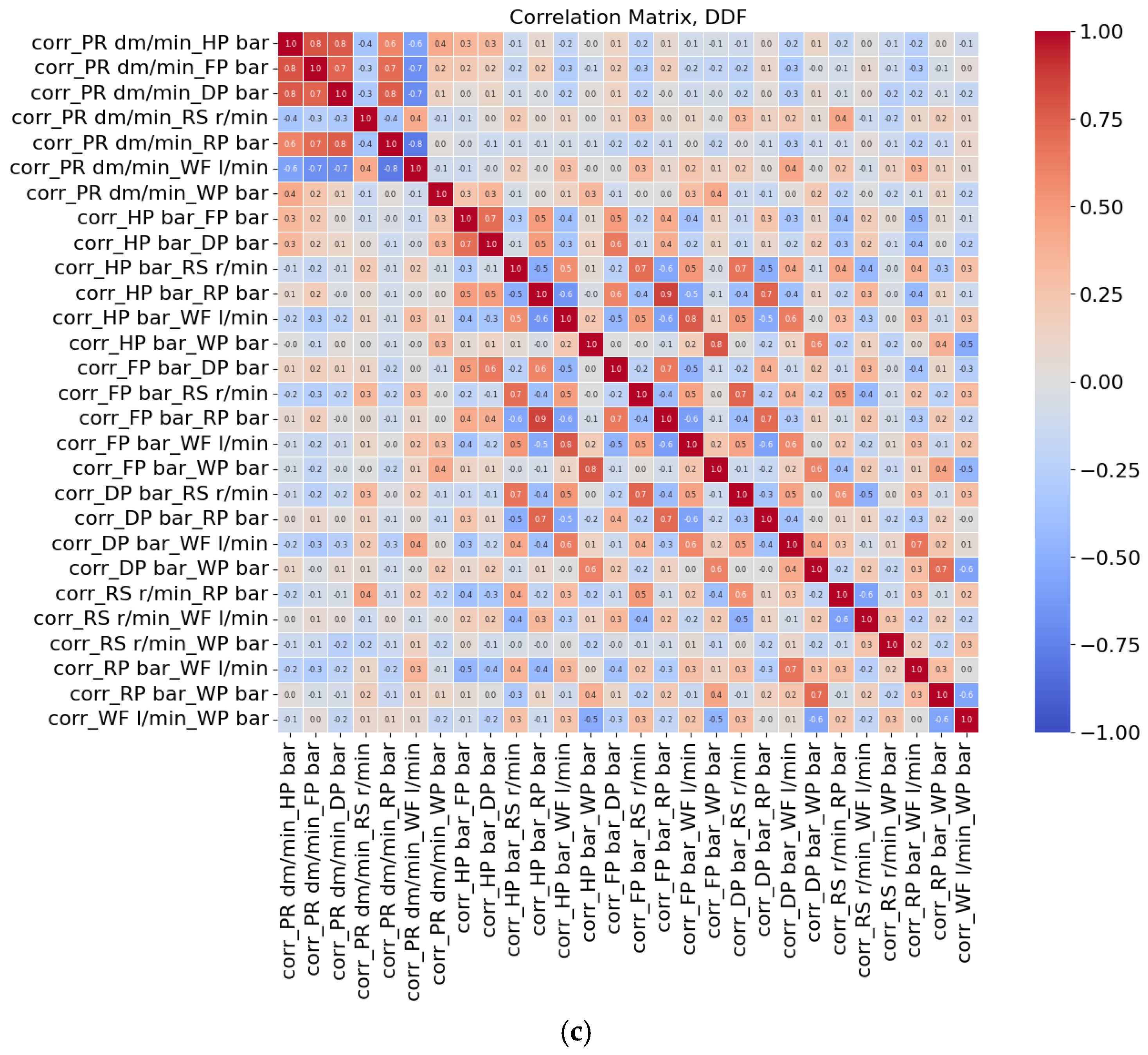
Figure 2 demonstrates how the amount of inter-correlation between variables in datasets (dark-colored cells) changes from DF to DDF.
As shown in the DF dataset (
Figure 2a), the variables exhibit a high degree of inter-correlation, with many features strongly correlated with each other. Given the limited number of features and their strong dependencies, it is unlikely that this dataset will yield a strong predictive performance in ML training. In contrast, the SDF (
Figure 2b) and DDF (
Figure 2c) datasets have more features and show a reduction in correlation due to the applied data pre-processing. The DDF dataset demonstrates the lowest inter-variable correlations, reflecting the effectiveness of the correlation-based feature derivation process for reducing the redundancy in data. This reduction in correlation in DDF indicates its potential to provide unique information for ML model training, potentially improving its ability to identify patterns in data.
After comparing the informational content of the three datasets, the DDF dataset was selected for ML model training. The approach used to construct DDF implicitly applies data normalization and dimensionality reduction procedures. The dimensionality reduction implies that instead of looking at the MWD time series for each hole (or a less informative average/min/max statistical description of these time series), we will end up with one row of correlation coefficients for each borehole. In addition, ML predictions trained on MWD offer complementary value by filtering out signals from noise and offering standardized predictions under variable conditions.
4.2. Building a Predictive ML Model
Following the data preparation stage, we train and test predictive MLMs to forecast the volume of explosives required for the contour holes.
To develop a robust predictive model, we initially considered multiple machine learning techniques, including linear regression, neural networks (NNs), and random forest regressor (RFR).
Linear regression was excluded due to its assumption of linear dependencies, which does not align with the complex, nonlinear relationships present in MWD data. The RFR was selected due to its ability to handle nonlinear relationships, resist overfitting, and perform well on datasets with mixed feature importance.
A simple NN (in the form of a multi-layer perceptron) was also tested; however, the NN-based model demonstrated lower performance on the available dataset compared to the RFR.
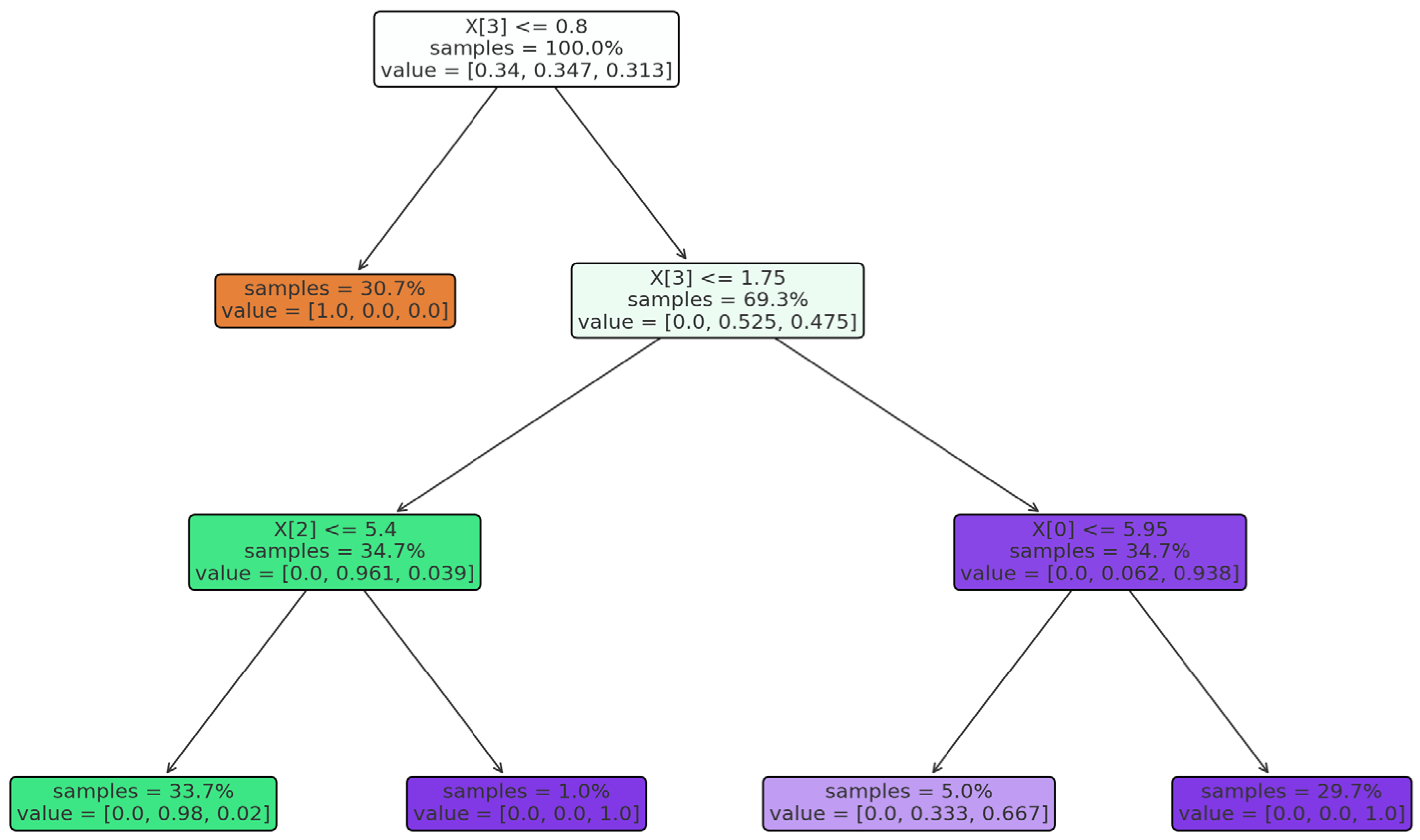
Random forest is an ensemble learning method that builds multiple decision trees and averages their predictions to reduce variance. Decision trees use a flowchart similar to a tree structure to show the predictions that result from a series of feature-based splits. It starts with a root node and ends with a decision made by leaves. Each tree is trained on a bootstrapped subset of the data, introducing randomness and improving generalization. Feature importance is determined by measuring the reduction in impurity (e.g., the Gini index or mean squared error) across all trees.
To better illustrate how the RFR generates predictions,
Figure 3 shows a conceptual diagram of the random forest architecture.
Table 2 shows the accuracy of the RFR model on the test datasets.
The RFR model trained on the DDF dataset showed the highest accuracy, suggesting the effectiveness of correlation-based feature engineering for capturing meaningful patterns within the data.
While the DDF dataset demonstrates advantages in terms of information richness and predictive accuracy, it is important to acknowledge potential limitations. Correlation-based features can be sensitive to residual noise or window size selection. Moreover, the increased dimensionality resulting from pairwise correlations can introduce risks of overfitting, particularly if regularization or dimensionality reduction is not applied. These concerns were mitigated in this work through the use of random forest and transformer models, which inherently manage high-dimensional data well, but further investigation may be needed in future applications.
The reduced noise and redundancy in DDF enable the model to “focus” on the most relevant features for prediction.
The model trained on the SDF dataset shows moderate accuracy, outperforming the model trained on the DF dataset but not achieving the accuracy of the DDF-trained model. This suggests that while statistical features (e.g., mean, min, and max) improve the dataset’s informativeness, they may retain more redundant or less predictive information than the derived features in DDF.
The outputs from the RFR model trained on the DF dataset show the lowest accuracy, indicating that the pre-processing routine applied to DF was not optimal for preparing the data for RFR model training. This also shows that advanced pre-processing steps are important to improve the quality and predictive skills of RFR models trained on MWD data.
To ensure the obtained results are applicable not only to the RFR type of ML models, we trained a more advanced NN model: a transformer-based model. Transformer-based ML models are a relatively new type of ML but are well known for their effectiveness. Recently, transformers have been adapted for use with tabular data through transfer learning techniques [
24]. The “RFR training/validation loss after 100 epochs” and “transformer training/validation loss after 100 epochs” metrics in
Table 3 show the values when each dataset was used for training.
The DDF dataset shows significantly lower validation losses for both the RFR and transformer models compared to the DF and SDF datasets. This indicates that the DDF dataset supports better generalization, allowing the models to predict unseen data more accurately.
The training loss for the RFR model is slightly higher for the ML model trained on DDF than the model trained on SD, but still shows lower validation loss. This suggests that DDF’s features reduce overfitting, leading to improved performance on validation data. Similarly, for the transformer model, DDF yields the lowest validation loss while maintaining competitive training loss, emphasizing its suitability for complex model architectures that require high-quality, non-redundant data.
To validate the observed performance differences, we used a Wilcoxon signed-rank test to compare the prediction errors of the models trained on DDF versus those trained on DF and SDF. The test results showed a statistically significant improvement in model accuracy using the DDF dataset (p < 0.01), confirming that the performance gains are unlikely due to random variation. These reinforce the conclusion that correlation-based pre-processing leads to more robust ML model training.
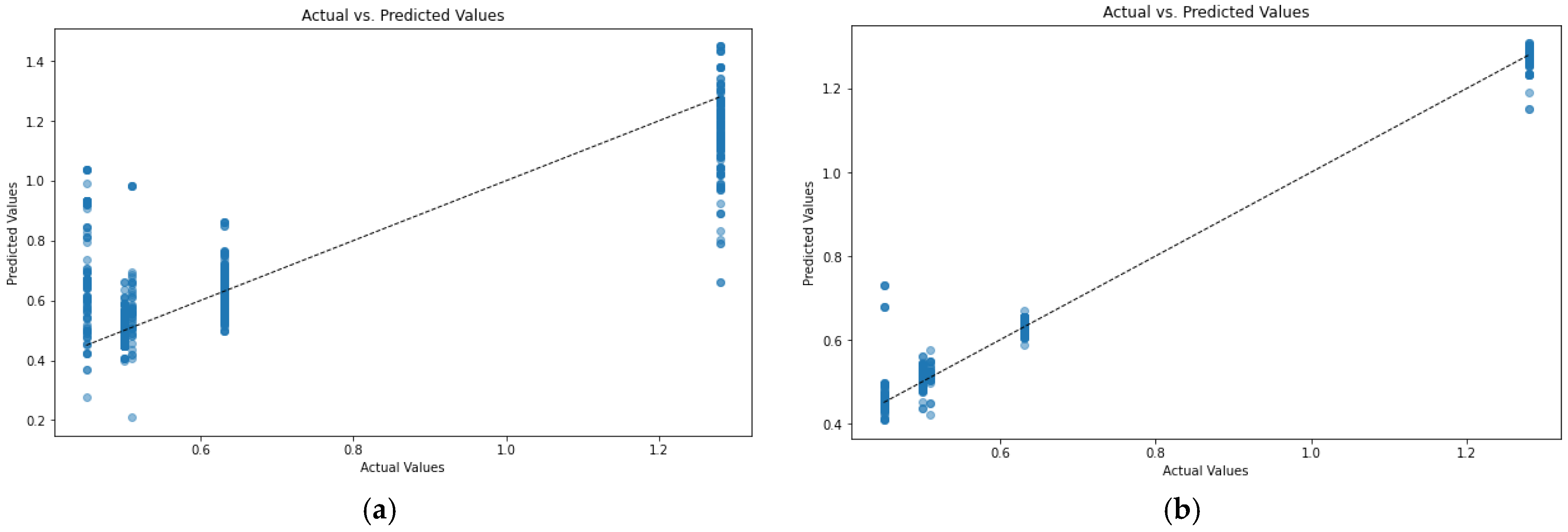
To finalize our comparison of ML models, we compared the prediction accuracy of RFR and transformer-based ML models, both of which were trained on the DDF dataset (
Figure 4).
This result clearly shows the advantage of the transformer-based models trained on the DDF dataset (which achieved the lowest validation loss among the three datasets). This means that the transformer models can better pick up the detailed information from the DDF dataset than the RFR and that transformer-based ML enables superior generalization.
5. Conclusions
This work presents a workflow for predicting the volume of explosives with ML models trained on pre-processed MWD data. It demonstrates how using correlation analysis aids in preparing the training dataset that provides more information to the ML models.
We demonstrate the advantages of using a derived dataset (DDF) for ML model training, particularly in predictive accuracy and robustness. DDF shows higher entropy, lower correlation among features, and reduced noise levels, and it provides richer informational content compared to the ML model’s original (DF) and statistical (SDF) datasets. The correlation-based feature engineering process effectively reduces redundancy in the data, which is indicated by the lower inter-feature correlations in DDF. Lower redundancy in DDF improves the ability of ML models to identify meaningful patterns and leads to more accurate predictions, as demonstrated by the performance of both RFR- and Transformer-based models.
The observed improvements in the DDF’s SNR indicate that the pre-processing routine minimizes background noise. This characteristic is particularly important in MWD data analysis, where inherent variability in rock mass conditions and drilling operations often introduces significant noise. The low number of outliers in the DDF dataset suggests that correlation-based feature engineering contributes to greater stability during model training.
The DDF dataset demonstrates higher dimensionality and the balance between feature complexity and relevance appears to be well-maintained, as shown by the reduced training and validation losses in both models. This indicates that the risk of overfitting due to high dimensionality is mitigated, likely due to the use of regularization techniques and the incorporation of non-redundant features. The improved performance of the transformer-based model on the DDF dataset highlights its ability to leverage the detailed, high-quality features provided by correlation-based engineering. The reduced validation loss observed in the transformer-based model suggests that advanced architectures benefit from datasets optimized for informational content and feature diversity.
The obtained results highlight the limitations of traditional pre-processing approaches. With its more traditional pre-processing, the DF dataset had the lowest predictive accuracy. Similarly, while the SDF dataset showed moderate improvements, its reliance on basic statistical metrics (mean, min, and max) appears insufficient for capturing the intricate relationships present in MWD data.
We also demonstrate that predictive models with transformer-based architecture outperform RFR models. The observed superiority of transformer-based models suggests that future research should focus on advanced architectures to fully exploit the richness of optimized datasets.
The proposed strategy for building ML models capable of predicting the volume of explosives can contribute to operational optimization by allowing a proactive approach to risk management, reducing the risk of over- or underbreak, and reducing the overall cost of tunneling projects.
We also explained the process of selecting a dataset for ML model training. The presented methodology for evaluating the amount of information in the dataset can be applied as a guideline to any dataset aimed at ML model training. The proposed approach for dataset selection allows us to avoid the commonly used, time-consuming trial-and-error approach to feature and dataset selection.
We showed the benefit of integrating ML with MWD correlation analysis rather than relying solely on direct interpretations of drilling logs. While MWD remains a crucial data source, its predictive value is substantially improved when coupled with statistical pre-processing and machine learning, enabling more reliable assessments of rock mass conditions and excavation requirements.
The dataset used in this study reflects real operational data from a single tunnel project. Future work should assess the model’s generalizability by training and testing on diverse geological settings, including class-balanced datasets across varying lithologies and borehole depths.
Future research shall also involve testing the proposed correlation-based pre-processing method on larger and more diverse datasets, including datasets from varying geological environments and different types of tunneling projects (e.g., TBM). Additionally, extending the methodology to incorporate dynamic time warping and unsupervised clustering for pattern detection may further improve the adaptability and robustness of ML models in geotechnical applications.


