Machine Learning-Enhanced Analysis of Small-Strain Hardening Soil Model Parameters for Shallow Tunnels in Weak Soil

Abstract

Accurate prediction of tunneling-induced settlements in shallow tunnels in weak soil is challenging, as advanced constitutive models, such as the small-strain hardening soil model (SS-HSM) require several input parameters. In this study, a case study was used as a benchmark to investigate the sensitivity of the SS-HSM parameters. An automated framework was developed, and 100 finite-element (FE) models were generated, representing realistic input ranges and inter-parameter relationships. The resulting distribution of predicted surface settlements resembled observed outcomes, exhibiting a tightly clustered majority of small displacements (less than 20 mm) alongside a minority of widely scattered large displacements. Subsequently, machine-learning (ML) techniques were applied to enhance data interpretation and assess predictive capability. Regression models were used to predict final surface settlements based on partial excavation stages, highlighting the potential for improved decision-making during staged excavation projects. The regression models achieved only moderate accuracy, reflecting the challenges of precise displacement prediction. In contrast, binary classification models effectively distinguished between small displacements and large displacements. Arguably, classification models offer a more attainable approach that better aligns with geotechnical engineering practice, where identifying favorable and adverse geotechnical conditions is more critical than precise predictions.

1. Introduction

The development of constitutive models that accurately predict soil behavior is a central challenge in geotechnical engineering research. While numerous sophisticated constitutive models have been proposed, their widespread validation across diverse geotechnical problems and conditions is limited [1]. The Hardening Soil Model (HSM) is an advanced constitutive model used in geotechnical engineering to capture the non-linear stress–strain behavior of soils. Schanz et al. [2] developed the framework for HSM and provided the mathematical formulation. The HSM improves upon simpler models, such as the traditional Mohr–Coulomb model, by incorporating stress-dependent stiffness and plastic strain hardening. The HSM has been shown to yield more realistic results for a range of geotechnical problems. The extended version, known as the Hardening Soil Model with Small-Strain Stiffness (SS-HSM), further refines predictions by considering stiffness degradation at small strains [3]. Incorporating small-strain stiffness into numerical models has been shown to enhance the accuracy of deformation predictions in geotechnical engineering.

The use of SS-HSM is particularly beneficial for modeling tunnels in soil, where small-strain effects significantly influence ground displacements. For example, Hsiung [4] simulated tunneling via a tunnel boring machine (TBM) through loose sands, demonstrating that SS-HSM provides more accurate predictions of ground deformations compared to traditional methods. Wang et al. [5] applied SS-HSM to model the impact of tunneling beneath pipelines and found that the simulated deformation of the pipelines was in agreement with the measured deformation. However, the application of SS-HSM is often limited due to the complexity and time-consuming nature of determining its numerous input parameters. In this study, a case study of a large, shallow tunnel excavated in weak cohesionless sand was modelled with SS-HSM.

This study builds on the methodology established in a previous paper by [6]. There, a comparative analysis of embedded wall displacements using SS-HSM was undertaken. An automated framework was utilized to compare multiple finite-element (FE) model results with empirical data from a large database provided by [7]. The same range of SS-HSM parameters was used to study tunnel behavior in sandy soils in the current study.

We used a case study of a large and shallow tunnel in sand as a benchmark case. The tunnel was constructed via conventional techniques, including staged excavation, forepole pipes, and jet grouting, to minimize volume loss and settlement. The baseline FE model is calibrated against monitoring data from this tunnel. The objective of the study was twofold: first, to assess the sensitivity of SS-HSM parameters on tunnel-induced ground displacements using a calibrated FE model; and second, to demonstrate how machine learning (ML) tools can be integrated with FE modeling practice. ML is a set of computational tools that learn patterns from data [8]. Coupling ML with FE modeling can be used for different purposes, including improving our understanding of model behavior and assessing predictive power, as demonstrated in the paper.

The paper is organized according to the following structure: first, we provide background information regarding SS-HSM. Second, we describe the case study project. Third, we provide the details of the FE modeling. Fourth, we outline the ML tools, which include regression and classification model, used to investigate the data obtained from the FE analysis. Finally, we summarize the main findings and conclusions.

2. The Small-Strain Hardening-Soil-Model

The SS-HSM extends the conventional HSM by incorporating strain-dependent stiffness degradation, making it particularly useful for capturing soil behavior under small-strain conditions. The key parameters for defining SS-HSM include:

• E₅₀ (secant modulus for primary loading)—Governs soil stiffness under deviatoric loading.
• E_oed (oedometer modulus)—Defines soil stiffness under one-dimensional compression.
• E_ur (unloading/reloading modulus)—Controls stiffness during unloading and reloading.
• G_ref (reference shear modulus at small strains)—Represents soil stiffness at very small strains.
• γ_0.7 (shear strain at 70% degradation of Gref)—Describes strain-dependent stiffness degradation.
• c (effective cohesion)—Governs shear strength.
• ϕ (effective friction angle)—A key parameter for soil shear strength.
• Ψ (dilatancy angle)—Defines volume expansion during shearing.
• m (power law parameter for stress-dependent stiffness)—Controls the nonlinear stiffness variation with confining pressure.
• K₀ (lateral earth pressure coefficient for normally consolidated soil)—Governs the initial lateral stress state.
• OCR (overconsolidation ratio)—Represents pre-consolidation history.
• p_ref (reference pressure)—A scaling parameter for stiffness dependency.

The stress-dependent parameters mimic the soil’s increased stiffness under small strains. The reference shear modulus Gref captures cyclic degradation of soils [9]. The unloading Eur captures soil behavior following excavation and reduces unrealistic floor heaving in simulations of tunnels and retaining walls [10]. The SS-HSM includes a hardening yield envelope that allows for a gradual transition from elastic to plastic behavior. Obrzud and Truty [11] provide a comprehensive review of HSM and SS-HSM and the various tests required for determining the values for the input parameters.

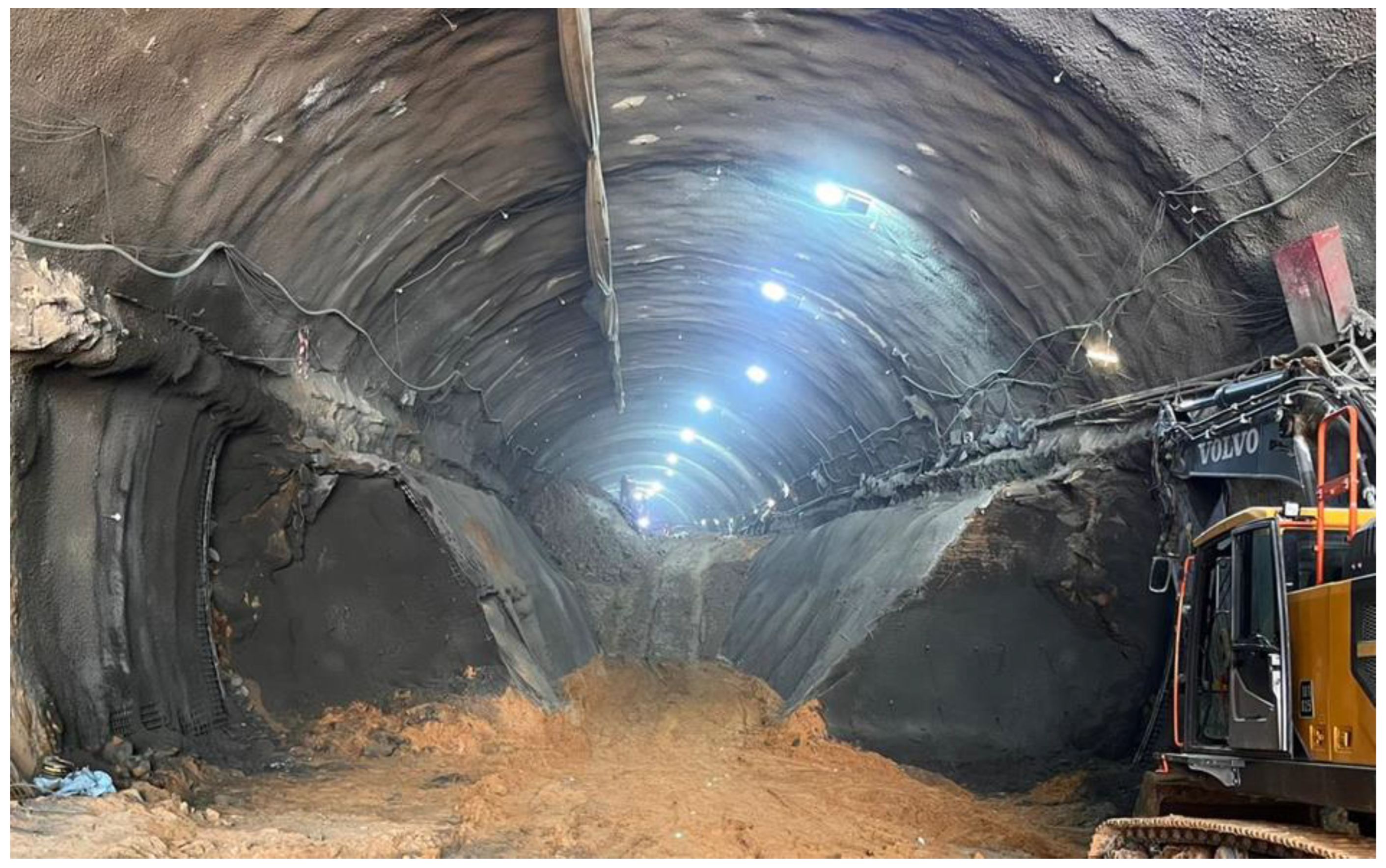
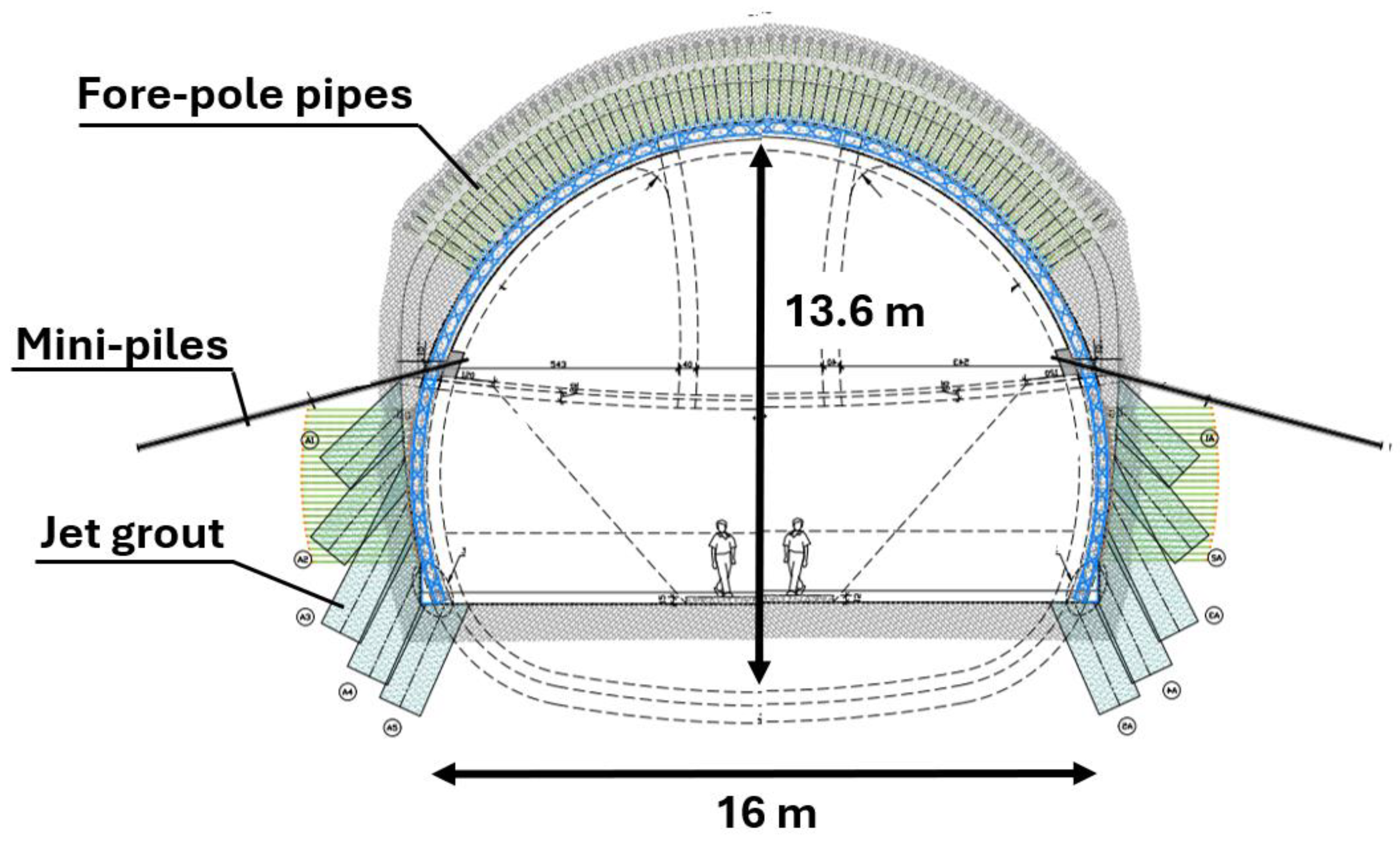
3. Case Study Information

The 431 railway project from Rishon LeZion to Modi’in and its connection to the fast line to Jerusalem is one of the largest and most complex infrastructure projects currently constructed in Israel. The line includes a large number of bridges and tunnels that will pass through the route. Along the planned route, near the city of Ramla, an ancient cemetery is located. Due to religious considerations, the cemetery imposed a constraint and did not allow for implementing the cut-and-cover method, that is favored for shallow tunnels. Hence, it was determined that this portion of the tunnel, referred to hereinafter as the 431-1 tunnel, would be constructed via conventional tunneling. The length of the 431-1 tunnel is approximately 250 m. The tunnel cross-section dimensions are 16 m in width and 13.6 m in height. Figure 1 shows the 431-1 railway tunnel under construction, prior to the excavation of the side drifts.

The tunnel’s location is approximately 5.5 km inland from the Mediterranean Sea. The shallow subsurface strata along this coastal region consist predominantly of aeolian deposits, specifically windblown sands and loess, which have been shaped by the fluctuating climatic conditions of the Pleistocene and Holocene epochs, as well as ongoing coastal processes [12]. These sands are derived from aeolian transport of sediments originating in the Sinai and Saharan deserts. This transport was particularly pronounced during colder, drier glacial periods, when sparse vegetation cover facilitated extensive wind activity. Conversely, warmer interglacial periods fostered soil stabilization and the accumulation of organic matter. From a geotechnical standpoint, the coastal sands exhibit low cohesion and high permeability, rendering them vulnerable to erosion and instability. While localized clay deposits, formed through a combination of aeolian, alluvial, and marine sedimentation processes, contribute to increased cohesion in certain areas, the primary tunneling hazard is posed by pockets of loose dune sand.

A comprehensive site investigation was conducted, and included standard penetration tests (SPT), cone penetration tests (CPT), sieve analysis for grain size distribution, direct shear tests, among other tests. SPT blow counts were in the range of 10–25 at depths between 0–10 m, and primarily in the range of 30–45 at depths between 10–30 m. The CPT tests indicate that the soil profile predominantly consists of medium to dense sands, characterized by relatively high cone resistance values, along with localized layers exhibiting a higher silt or clay content. The sieve analysis results also indicate that the soil predominantly consists of sand, ranging between approximately 70% to 96%, accompanied by varying amounts of silt and clay, with no gravel present. Direct shear tests yielded friction angles in the range of 31–34° and cohesion values of 2–23 KPa. Jet-grouted core samples were taken from the site and tested in the laboratory. These tests showed that the grouted soils have variable unconfined compressive strengths ranging from approximately 3.0 MPa to 8.8 MPa, and Young’s modulus values ranging from about 12 to 14.5 GPa.

The case study project is particularly risky and challenging due to a number of its main features. First, shallow tunnels lack sufficient overburden for effective arching, thus increasing stresses and deformations [13]. Second, tunnels passing through uncemented sands presents a risk of sand inflow into the tunnel excavation, potentially triggering instability and collapse, excessive surface settlement, and sudden formation of sinkholes [14]. Third, the large dimensions of the tunnel further exacerbate these risks, as a wider excavation span can result in greater stresses and deformations, and the risk of uncontrolled sand flow increases.

Given these risks, devising the appropriate excavation sequencing and support measures is crucial. Figure 2 shows an illustration of the tunnel support measures. The excavation is sequenced, with the top portion relying on a dense array of forepole steel pipes and a 40-cm thick concrete lining with lattice girders. Face stability is crucial for these types of tunnels, and therefore, shotcrete and fiberglass nails are applied at the tunnel face. The deepening of the tunnel (i.e., bench) is applied after some advance has been made in the top portion in order to reduce the risk of face collapse. To guarantee the stability of the tunnel in the lateral direction, prior to the deepening excavation stages, 11 m long mini-piles were installed at both sides every 50 cm. In addition, jet grout was applied to reduce the risk of sand flow. The deepening was divided into mid and side drifts, and temporary shotcrete was applied prior to each stage of excavation (see Figure 1). A final invert lining was constructed in order to close the structural load-bearing system and form a compressive ring, thus ensuring long-term stability.

The project is currently in progressive stages of construction. The greatest challenge encountered has been managing the unpredictable flow of pockets of dune sand, which, in some cases, leaked rapidly into the excavation before the installation of support measures. This unexpected sand inflow posed a significant stability risk, which was manifested by excessive surface settlement. A learning curve has been developed throughout the excavation to refine the support system and optimize stabilization techniques.

It is important to emphasize that while the focus of this paper is on FE modeling and data analysis, these alone cannot replace a fundamental understanding of geotechnical risks and potential failure mechanisms. Numerical tools are only as valuable as the engineering judgment that underpins them [15].

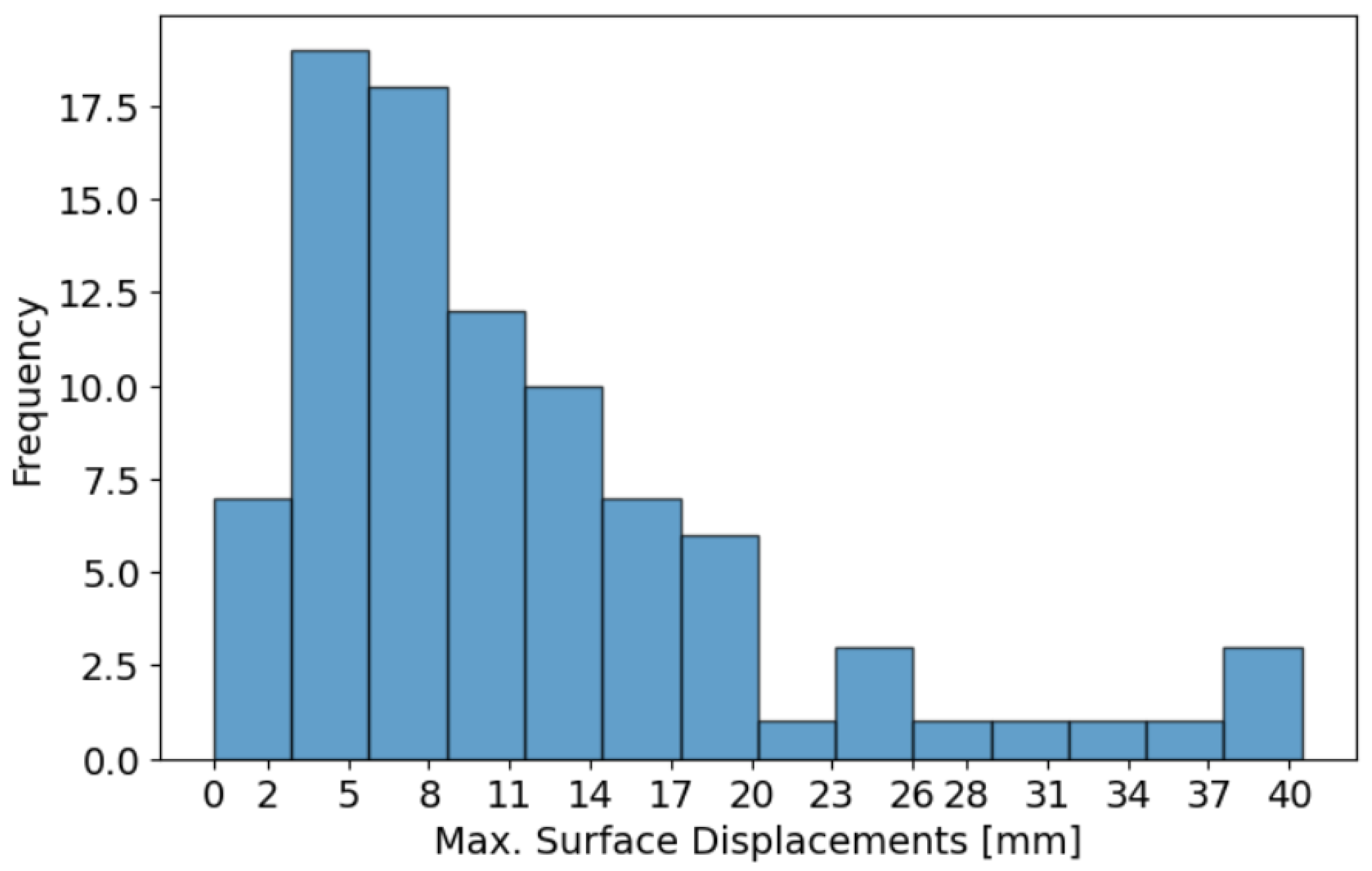
4. Finite-Element Modelling

A baseline FE model of the 431-1 tunnel was built using RS2 [16]. The model was divided into 12 construction stages corresponding to the tunneling sequence. These stages included initial ground conditions, application of surcharge load, top excavation, top liner installation, mini-pile installation, jet grouting, middle drift, side excavations, side liners, lower excavation, and invert liner (see Figure 2 and Figure 3). The surcharge load was assigned a moderate value of 0.01 MN/m² to account for pedestrian flow and cemetery infrastructure. The forepole pipes were not simulated directly, as they serve an intermediate purpose and do not contribute to the final stiffness of the support system. Instead, the induced stress feature from RS2 was applied during the top excavation stage, where stresses that are equal in magnitude and opposite in direction to the actual stress on the tunnel boundary are assigned. A factor of 0.8 was assumed for these stresses, as the forepole pipes allow for some displacement to occur.

Table 1. Input parameters for the support system.

Support Element	Input Parameter	Value
Tunnel liner	Thickness [cm]	40
	Young’s modulus [MPa]	30,000
	Poisson ratio [-]	0.2
Temporary tunnel invert	Thickness [cm]	35
	Area (m2)	30,000
	Poisson ratio [-]	0.2
Temporary side liner	Thickness [cm]	10
	Young’s modulus [MPa]	30,000
	Poisson ratio [-]	0.2
Inclined pile	Young’s modulus [MPa]	200,000
	Area [m2]	0.000484
	Spacing [m]	0.6
	Poisson ratio [-]	0.25
Jet Grout	Young’s modulus [MPa]	1400
	Poisson ratio [-]	0.3
	Friction angle (degrees)	34
	Cohesion (MPa)	0.93

lists the input parameters of the support system. The Young’s modulus and Poisson ratio for concrete and steel are based on standard engineering values, and the jet grout parameters are based on laboratory tests of samples extracted from the site.

To enhance computational efficiency, only half of the problem domain was modeled, taking advantage of the tunnel’s geometric symmetry. A vertical symmetry plane was introduced along the tunnel centerline, where displacement constraints were applied using vertical rollers to allow vertical settlement and rotation while preventing horizontal movement. As part of the preliminary work, the half model was compared to the full model to verify that stress and displacement results are consistent. Additional preliminary investigations included a mesh sensitivity analysis. Figure 3 shows the FE half model geometry, special support components, and excavation sequence.

A key parameter for tunneling-induced surface settlement predictions is volume loss [17]. Empirical methods that estimate surface settlements based on volume loss typically apply to deeper tunnels that resemble most metro lines [18]. For FE modeling, there are several methods for incorporating volume loss into the simulation [19]. For example, the contraction ratio method applies a uniform radial contraction to the tunnel boundary, simulating volume reduction due to excavation. The gap parameter method introduces a predefined gap at the tunnel crown to account for excavation-induced voids. In the current case study, volume loss was considered negligible due to construction techniques that mitigated over-excavation. These included forepole pipes, jet grouting, and face stabilization via shotcrete and fiberglass nailing. Thus, surface displacements in this analysis were assumed to be primarily governed by the tunnel crown displacement. The FE model results therefore reflect a lower-bound estimate of the actual displacements. In some instances, the surface settlement was significantly larger, and these were associated with effects of rapid sand flow and volume loss.

Coupling FE modeling with external software offers significant advantages for automating the generation and analysis of numerous models. This approach facilitates the workflow by assigning parameter variations and applying data analysis tools. A total of 100 FE models were generated by varying SS-HSM soil parameters based the input ranges and relationships listed in

Table 2. Assumed SS-HSM input parameters statistical ranges and relationships.

Parameter	Unit	Min	Max	Relationship
$E_{50}^{ref}$	[MPa]	1	150
$E_{oed}^{ref}$	[MPa]	0.5	225	$0.5<{\displaystyle \raisebox{1ex}{$E_{oed}^{ref}$}\!\left/ \!\raisebox{-1ex}{$E_{50}^{ref}$}\right.}<1.5$
$E_{ur}^{ref}$	[MPa]	1	1575	$2.0<{\displaystyle \raisebox{1ex}{$E_{ur}^{ref}$}\!\left/ \!\raisebox{-1ex}{$E_{50}^{ref}$}\right.}<7$
$\mathrm{m}$	[-]	0.5	1
υ	[-]	0.2	0.3
$K_0^{NC}$	[-]	0.4	0.6
ϕ	[Deg]	20	40
Ψ	[Deg]	0	10	ϕ-30°
cohesion	[MPa]	0	0.01
Rf	[-]	0.6	0.9
ψ	[Deg]	0	10
$G_0^{ref}$	[MPa]	1.1	2677.5	$1.1<{\displaystyle \raisebox{1ex}{$G_0^{ref}$}\!\left/ \!\raisebox{-1ex}{$E_{ur}^{ref}$}\right.}<1.7$
${\gamma }_{0.7}$	[-]	0.0001	0.001

. In this table, various inputs are varied directly, while other inputs are varied according to empirical findings given by [20]. For example, E_ur, the unloading modulus, is known to be significantly larger than E₅₀ and, therefore, assigned a value increased by a factor of 2–7. The relationship between the shear modulus G_ref and E_ur was also limited to a range of 1.1–1.7. A Python script was used to create the input data table and automate model generation.

Following the completion of model solving, another script extracted the maximum surface settlement that occurred above the tunnel centerline from each FE model. A histogram of the surface displacement results is shown in Figure 4. For clarity, a number of extremely large displacements were removed from this plot. These outlier results occurred in non-converging models, which indicate a potential for loss of stability and failure. The histogram indicates that the majority of settlements are relatively small, typically ranging from a few millimeters to 20 mm. The predominance of small displacement results is consistent with typical SS-HSM predictions, which account for the stress-dependent stiffness behavior of soils and their gradual deformation under loading. This finding also aligns with observed tunnel construction outcomes, where under standard conditions most tunnels experience limited surface settlements. This outcome is similar to the earth-retaining wall displacements, where the vast majority of displacements are small [7]. The observed surface settlements for the case study tunnel were approximately 40–50 mm. This aligns with the assumption that the soil at the case study is at the weak end of the spectrum.

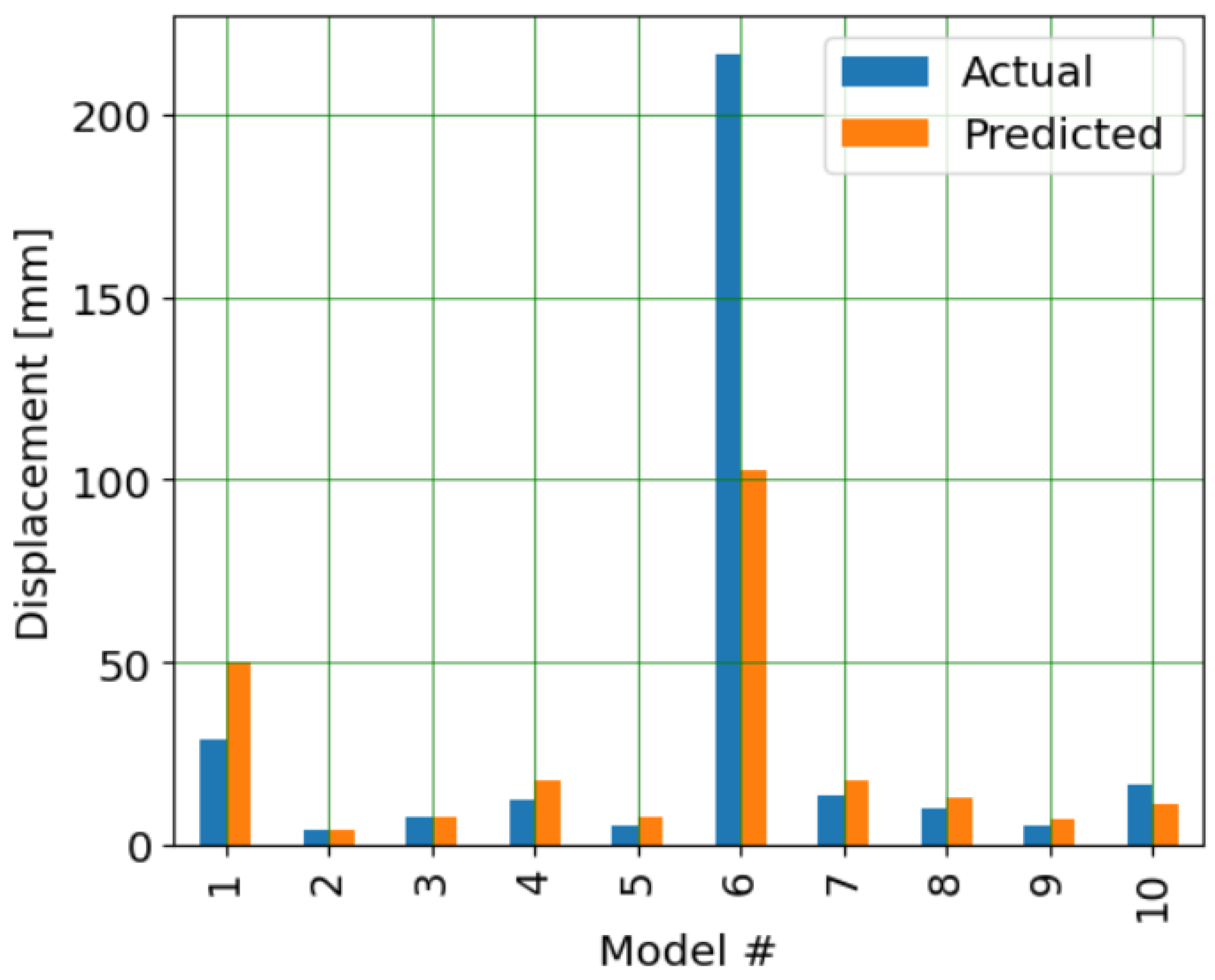
5. Machine-Learning Analysis

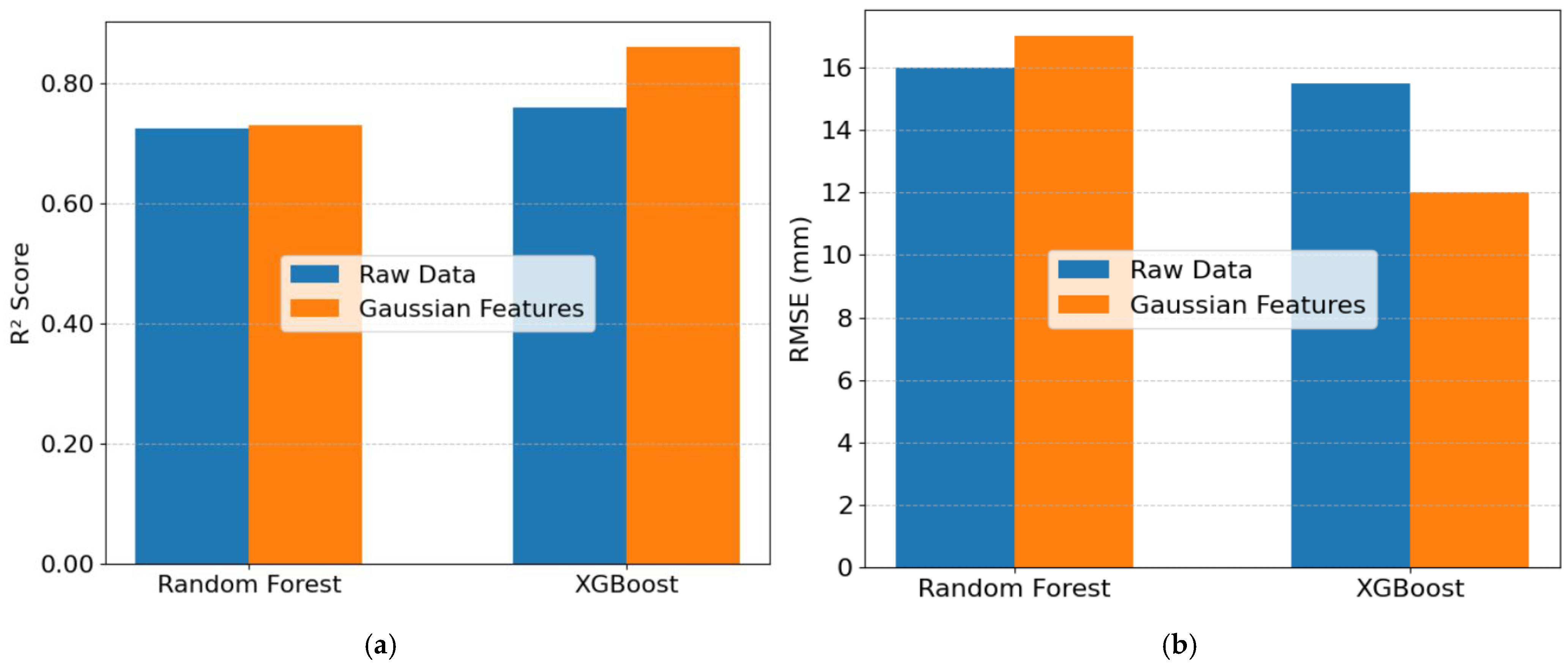
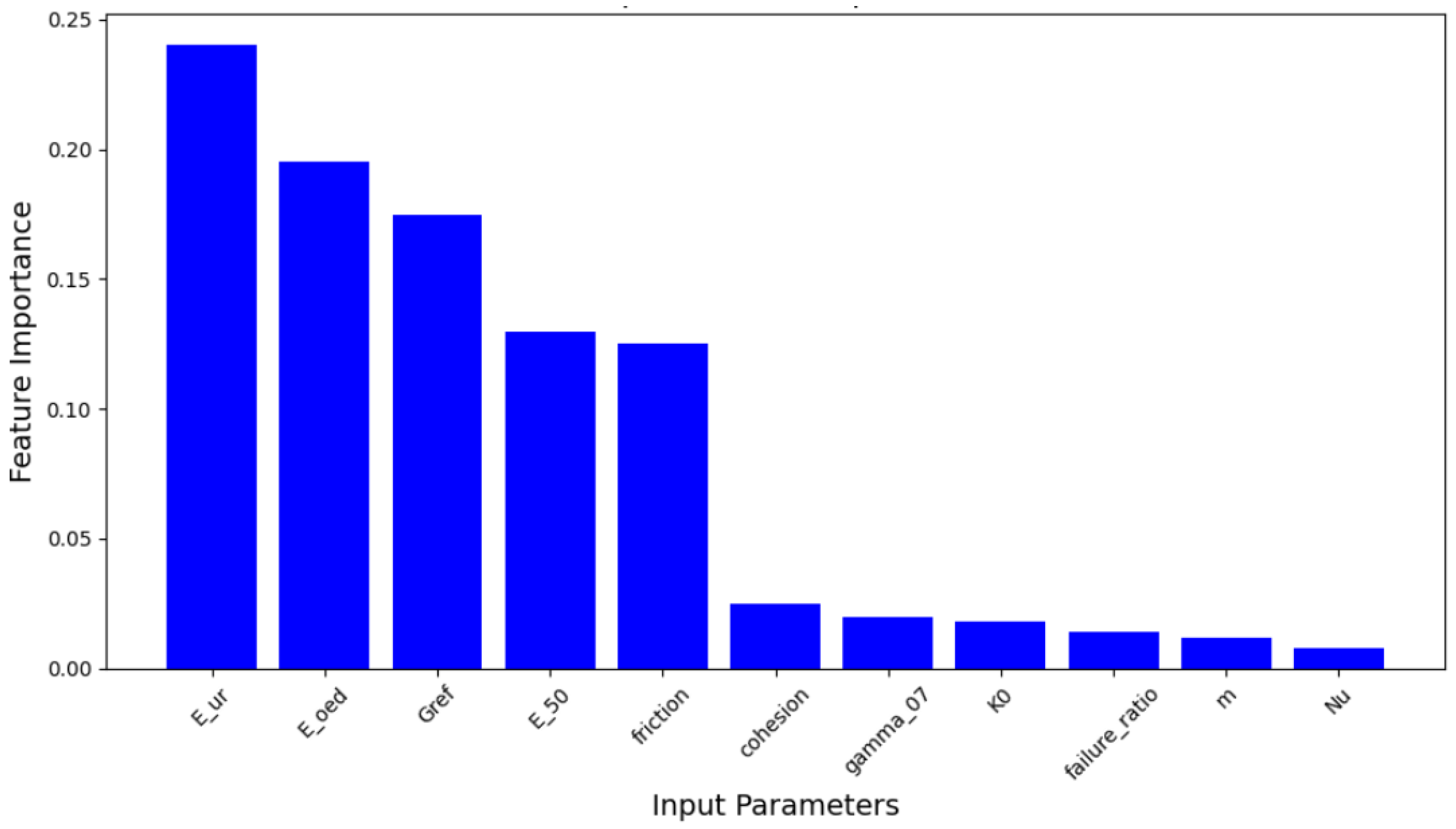
5.1. Regression Models

Regression models in ML are aimed at correlating input features with numerical outputs, a process referred to as training. A random forest (RF) regression model was trained to correlate SS-HSM parameters with maximum displacement values. RF is an ensemble learning method that constructs multiple decision trees and averages their outputs, enhancing predictive robustness while reducing overfitting [21]. Compared to neural networks, RF is often preferred for many engineering applications due to its ability to handle small datasets effectively and lower computational cost, making it well-suited for geotechnical problems where nonlinear parameter interactions must be understood [22]. The ML models in this study were implemented using the Scikit-learn (sklearn) library, which provides a robust framework for classification and regression tasks in engineering applications. The artificial intelligence (AI) tool ChatGPT version 4o was used for assistance with writing the scripts for the ML analysis.

Hyperparameters are adjustable parameters in machine learning models that define their structure and learning processes. An additional advantage of RF models is their low sensitivity to hyperparameter tuning, simplifying model development. In this study, the RF models were consistently configured with 500 decision trees to enhance prediction robustness, and a fixed random state to ensure reproducibility.

The train–test split is a fundamental part of ML, essential for performance evaluation and preventing overfitting [8]. A train–test ratio of 75:25 was used for all ML models in this study. For evaluation of ML model performance, there are different metrics available. For the regression models in this paper, we use R² and root mean squared error (RMSE) due to their widespread adoption. R² quantifies the proportion of variance in the target variable explained by the model, with a value of one indicating a perfect fit. RMSE measures the average difference between predicted and actual values, where lower values indicate greater predictive accuracy [23]. R² is a unitless score, and RMSE is in the units of the problem [8].

Overall, the regression model yielded a coefficient of determination R² of 0.67 and a relatively high RMSE of 23 mm. Figure 5 presents a comparison between predicted and actual tunnel displacements across a representative sample of ten randomly selected FE models. The results indicate that while the general trend is regularly being captured, there is a systematic under-prediction of large displacements. This is particularly evident in Model #6, where the actual displacement exceeds 200 mm, while the predicted value remains significantly lower. This discrepancy likely stems from an imbalance in the dataset, where the majority of observed displacements are relatively small (see Figure 4). As a result, the model is biased toward lower values, failing to capture outlier conditions with extreme displacements.

Considering that there are 12 varied input parameters for the SS-HSM and that there are only minor differences between the small displacements, accurate prediction becomes a difficult task. This suggests that a larger data set might be needed for improved accuracy. However, due to the inherent uncertainty of geological materials, achieving high accuracy is likely unrealistic.

Another application of regression models in staged geotechnical projects is predicting final tunnel-induced displacements using partial displacement data. In the case study project, we demonstrated this approach by using settlement profiles recorded after the top excavation stage to predict the final settlement profile.

For the ML model, we collected vertical settlement results from the FE models. The displacement profile following Stage #4 in the FE model (top excavation) was used as the input, while the final displacement profile recorded after Stage #11 (final stage) served as the target output. The displacement profile consisted of vertical displacement results from 38 nodes that spanned 24 m. Unlike the previous ML application in this study, where soil parameters were directly used as inputs to predict a single maximum displacement value, the present approach treated the output as an array of displacement values, representing a full settlement profile rather than a single numerical prediction. In this case, the SS-HSM parameters were implicit rather than direct inputs in the ML process. This shift in approach allows the ML model to learn from displacement trends rather than material properties, making it potentially more adaptable to cases where soil parameters are uncertain or unavailable and predictions are made based on actual soil behavior.

While this analysis is currently demonstrative, such an approach could have significant real-world benefits. If reliable, it could be used to forecast final settlements based on the monitoring data from earlier stages, improving risk management and decision-making during tunneling projects. However, several challenges must be addressed before deploying this method in practical applications. In FE simulations, an unlimited number of models can be generated, allowing for extensive training datasets. In real projects, monitoring data are sparse, as instrument installation is constrained by cost, site accessibility, and logistical factors. In addition, field monitoring data are subject to external disturbances, including construction vibrations, environmental factors, and instrumentation errors. Finally, real-world monitoring data requires continuous collection, cleaning, and interpretation.

Given these limitations, a potential solution is to leverage synthetic data from numerical models as a preliminary training step. Techniques, such as transfer learning, could then be applied to fine-tune models using limited real-world data, improving generalization while addressing data scarcity and noise issues.

To evaluate the feasibility of using ML for settlement profile prediction, 2 ML models were trained and tested against the dataset: (1) an RF regression model, and (2) the XGBoost model. XGBoost is a more advanced ML model, which includes a process of sequential learning, as well as a parallel computation, and a more sophisticated objective function that optimizes for both accuracy and execution speed [24]. For the RF models, the same hyperparameters described previously were applied. The XGBoost regression models were configured with 300 estimators, a learning rate of 0.05 to balance convergence speed with prediction accuracy, and a fixed random state ensuring reproducibility.

The RF model achieved an R² score of 0.725 and a RMSE of 16 mm. The XGBoost model achieved an R² score of 0.76 and a RMSE of 15.5 mm. Figure 6 shows an example of a single settlement profile, where the partial settlements, final settlements, and predictions by the RF and XGBoost models are plotted. As can be seen in Figure 6, in this example, both the RF and XGBoost models over-predicted the final settlements, where the over-prediction was very slight at the tunnel centerline, and the deviations increased farther away. It can also be observed that the predictions of the XGBoost were closer and more jagged. This is likely due to its sequential process, which makes it more sensitive to individual points, thus leading to a closer fit at the cost of smoothness.

Another approach was examined, where rather than using the displacements results themselves, key features of the settlement profiles were extracted. This process is referred to in ML terminology as feature engineering, where the data is transformed into meaningful features, potentially improving ML performance. In this process, a half-Gaussian curve-fitting function was applied to the displacement profiles. Subsequently, four parameters were extracted from each Gaussian curve: the maximum settlement, the median settlement, the decay length, and the baseline offset. The decay length indicates how quickly the curve reduces from its maximum values, and the baseline offset is constant, which shifts the curve vertically.

The RF and XGBoost regression models were trained on the Gaussian features. In order to evaluate and compare the performance of the ML models on the raw displacement data and the Gaussian parameters, the latter were used to transform the features back to Gaussian curves. This allows computing RMSE in a meaningful manner, where the deviations in displacement predictions are computed along each profile.

Figure 7 shows a bar plot that summarizes the performances of the RF and XGBoost models on the raw displacement data and Gaussian features. As can be seen in Figure 7, the RF model achieved an R² of 0.73 and an RMSE of 17 mm when trained on the Gaussian features. This showed a slight improvement in explanatory power over the raw data model and a marginally higher error (RMSE = 16 mm).

In contrast, XGBoost showed a marked improvement with Gaussian features, reaching an R² of 0.86 and an RMSE of 12 mm, compared to R² = 0.76 and RMSE of 15.5 mm for the raw data. This suggests that XGBoost effectively leverages the simplified, structured representation of settlement profiles provided by Gaussian features. These results indicate that by applying feature engineering and using the Gaussian parameters, model accuracy and variance explanation are enhanced, particularly for XGBoost. This highlights the benefit of incorporating physically meaningful features in ML models for displacement analysis.

5.2. Classification Models

Unlike regression, where the goal is to estimate a specific value, classification aims to assign data points to predefined categories or classes. In many cases, a continuous numerical outcome can be discretized into defined intervals, allowing regression and classification to be used interchangeably depending on the problem at hand. The performance of classification models is typically evaluated using metrics, such as accuracy, precision, recall, and the F1 score [23]. Accuracy provides an overall measure of percentage of the correct classifications. However, when viewed alone, it can be misleading when dealing with imbalanced datasets. For the current example, where large displacements constituted 10% of the dataset, a model can simply guess small displacements for all instances and achieve 90% accuracy. Precision quantifies how many of the predicted positive cases were actually positive, while recall measures how many of the actual positive cases were correctly identified. The F1 score, being the harmonic mean of precision and recall, provides a balanced measure that considers both metrics, especially useful when dealing with imbalanced class distributions.

Arguably, classification models align well with geotechnical projects, particularly observational method projects. In these projects, such as the current conventional tunneling project, engineers must assess a small number of different classes of ground conditions and make contingency plans for each of them. The support measures and tunnel sequencing are applied accordingly during construction based on the encountered condition at each step. Hence, predicting the actual displacement would be superfluous. Moreover, while it is possible to run thousands of FE models and achieve higher predictive accuracy, this accuracy does not align with predictive power in real-world geotechnical scenarios.

Accordingly, a classification approach was adopted. It was determined that a binary classification model would be used, i.e., that the displacements would be divided into only two classes. The reasons for this are twofold: (1) this histogram analysis reflected a binary division, with a 20-mm threshold dividing between small and large displacements (see Figure 4). (2) A constant sequencing and support scheme was devised for the project, where additional measures, such as extra grouting, were employed if extremely poor conditions were encountered. This division of probable vs. adverse ground conditions corresponds to the binary classification.

Since small displacements dominated the dataset, a multi-round training process was implemented to balance the classes. In each round, a distinct subset of small displacement cases was selected alongside the full set of large displacement cases, ensuring that the classifier encountered a diverse range of training samples. This process was repeated 5 times, each time progressively refining the RF model’s decision boundaries, thereby improving its ability to generalize to unseen data. With each successive round, the classifier exhibited enhanced predictive stability, mitigating its inherent bias toward the dominant class. The staged training methodology resulted in incremental improvements in accuracy, recall, precision, and F1 score. The final classification results showed an overall accuracy of 87.5%, with precision values of 0.75 and 1.0 for small and large displacement classes, respectively. Recall values were 1.0 for small displacements and 0.8 for large displacements, leading to F1 scores of 0.86 and 0.89 respectively. The macro-averaged precision, recall, and F1 score were 0.875, 0.9, and 0.87, respectively, indicating that the model effectively distinguished between the two displacement categories despite inherent data imbalances.

Another ML model was developed to classify whether an FE model would converge. Among the 100 models, 11 failed to converge. An RF classifier was trained on this dataset but failed to achieve reliable predictive performance, likely due to the small sample size of non-converging models.

From the RF model for small vs. large displacements, feature importance was computed to identify the SS-HSM parameters that have the greatest impact on displacement results. Feature importance is determined by measuring the change in model performance when a feature’s values are randomly shuffled. As can be observed in Figure 8, the Young’s moduli, E₅₀, E_oed, and E_ur had the highest influence on displacements. The shear reference modulus G_ref and friction angle also contributed significantly, and the other parameters had minor influence.

Feature importance results can assist in determining which field and laboratory tests should be prioritized. However, these results should be interpreted cautiously, as the ML model is not perfectly accurate. Such results should therefore be viewed as a preliminary indication that still requires further examination and validation. Moreover, feature importances are based on the unique assumptions, namely, the case study geometry and the assumed input parameters ranges, and therefore, conclusions should not be extended to other problems.

To further understand the displacement classification, two scatter plots were generated based on the impactful inputs as inferred from the feature importance analysis. The scatter plots in Figure 9 show what combination of parameters have resulted in small vs. large displacements, represented by blue and red dots, respectively. Figure 9a shows a plot of E₅₀ vs. G_ref, and Figure 9b shows a plot of E₅₀ vs. the friction angle. As anticipated, both scatter plots show that the majority of combinations that lie within the lower range of both parameters belong to the large displacement category. However, some outliers exist for both small and large displacements. The apparent reason for these outliers is that there are several other input parameters that influence the final outcome of the FE analysis. Nonetheless, based on these trends, it is likely that when selecting E₅₀ values below 50 MPa, G_ref values below 400 MPa, and friction angle values below 30°, the analysis outcome would fall within the large displacement category. While not definitive, such scatter plots provide guidance for selecting SS-HSM parameters that reflect favorable vs. adverse conditions. It is noted that when ML performance is sufficiently accurate, the ML model can act as a surrogate model that obviates the need for running additional time-consuming models [25].

6. Summary and Conclusions

This study uses the benchmark 431-1 tunnel case to evaluate the performance of SS-HSM in predicting tunnel-induced ground displacements by integrating ML tools with FE modeling. Investigating for a range of SS-HSM parameters found a majority of small displacements with few instances of large movements, similar to the observed reality in the case study tunnel. In addition, this aligns with findings from a previous study of SS-HSM parameter variation influence on embedded earth-retaining wall displacements [6,7].

Two types of regression models were developed. The first used a RF model aimed to correlate SS-HSM input parameters with surface displacement results. This regression model fell short of achieving high accuracy (R² = 0.67). This shortcoming likely arises due to the minor deviations among small displacement cases and the imbalance in the dataset. The second regression model involved predicting final displacements from full excavation based on partial displacements recorded after top excavation. RF and XGBoost models were used for this purpose. It was found that when the raw displacement profiles were transformed into Gaussian features the performance of the XGBoost ML model improved significantly (R² = 0.86).

A binary classification ML approach was implemented to differentiate between small (≤20 mm) and large (>20 mm) displacements. An iterative training process was employed to address the imbalance between these two classes by using distinct subsets of small displacement cases alongside all large displacement cases. This approach effectively improved model performance, yielding an accuracy of 87.5% and an F1 score of 0.87. Feature importance analysis identified key SS-HSM parameters, such as E₅₀, E_oed, G_ref, and E_ur, as primary influencers, and the friction angle as a secondary feature. Arguably, this method is more relevant for geotechnical decision-making, which regularly requires determining the relevant class of ground behavior rather than predicting precise displacements.

The reliance on a single case study imposes a limitation of the conclusions, as geotechnical behavior can vary significantly depending on site-specific factors. Another significant limitation of the modeling process is that the phenomena of volume loss and sand flow were not accounted for. Future research should focus on integrating ML techniques with real-world monitoring data, ultimately aiming to enhance risk management during staged excavation projects.

References

1. Lees, A. Geotechnical Finite Element Analysis; ICE Publishing: London, UK, 2013; ISBN 0727760874. [Google Scholar] [CrossRef]
2. Schanz, T.; Vermeer, P.A.; Bonnier, P.G. The Hardening Soil Model: Formulation and Verification. In Beyond 2000 in Computational Geotechnics; Routledge: London, UK, 1999; Volume 1, pp. 281–296. [Google Scholar]
3. Huynh, Q.T.; Lai, V.Q.; Boonyatee, T.; Keawsawasvong, S. Verification of Soil Parameters of Hardening Soil Model with Small-Strain Stiffness for Deep Excavations in Medium Dense Sand in Ho Chi Minh City, Vietnam. Innov. Infrastruct. Solut. 2022, 7, 15. [Google Scholar] [CrossRef]
4. Hsiung, B. Numerical Investigation of the Three-Dimensional Performances of a Shield-Machine-Bored Tunnel in Loose Sands. Soil Mech. Found. Eng. 2020, 56, 427–435. [Google Scholar] [CrossRef]
5. Wang, Y.; Kong, L.; Wang, Y.; Li, X. Analysis of Influence of Shield Tunneling on Overlying Underground Pipelines Based on HSS Model. IOP Conf. Ser. Mater. Sci. Eng. 2018, 423, 012017. [Google Scholar] [CrossRef]
6. Eilat, T.; Mitelman, A.; McQuillan, A.; Elmo, D. A Comparative Study of Embedded Wall Displacements Using Small-Strain Hardening Soil Model. Geotechnics 2024, 4, 309–321. [Google Scholar] [CrossRef]
7. Long, M. Database for Retaining Wall and Ground Movements Due to Deep Excavations. J. Geotech. Geoenviron. Eng. 2001, 127, 203–224. [Google Scholar] [CrossRef]
8. Kelleher, J.D.; Tierney, B. Data Science; MIT Press: Cambridge, MA, USA, 2018; ISBN 0262347032. [Google Scholar]
9. Castellon, J.; Ledesma, A. Small Strains in Soil Constitutive Modeling. Arch. Comput. Methods Eng. 2022, 29, 3223–3280. [Google Scholar] [CrossRef]
10. Obrzud, R.F. On the Use of the Hardening Soil Small Strain Model in Geotechnical Practice. Numer. Geotech. Struct. 2010, 16, 1–17. [Google Scholar]
11. Obrzud, R.; Truty, A. The Hardening Soil Model a Practical Guidebook; Zace Services Ltd.: Preverenges, Switzerland, 2018. [Google Scholar]
12. Roskin, J.; Sivan, D.; Shtienberg, G.; Roskin, E.; Porat, N.; Bookman, R. Natural and Human Controls of the Holocene Evolution of the Beach, Aeolian Sand and Dunes of Caesarea (Israel). Aeolian Res. 2015, 19, 65–85. [Google Scholar] [CrossRef]
13. Zhang, Z.; Li, H.; Yang, H.; Wang, B. Failure Modes and Face Instability of Shallow Tunnels under Soft Grounds. Int. J. Damage Mech. 2019, 28, 566–589. [Google Scholar] [CrossRef]
14. Hong, Q.; Lai, H.; Liu, Y. Failure Analysis and Treatments of Collapse Accidents in Loess Tunnels. Eng. Fail. Anal. 2023, 145, 107037. [Google Scholar]
15. Mitelman, A.; Yang, B.; Elmo, D.; Giat, Y. Choosing between Prediction and Explanation in Geological Engineering: Lessons from Psychology. Interdiscip. Sci. Rev. 2023, 48, 651–668. [Google Scholar] [CrossRef]
16. Rocscience Phase2 Version 6.020; Rocscience Inc.: Toronto, ON, Canada, 2007.
17. Peck, R.B. Advantages and Limitations of the Observational Method in Applied Soil Mechanics. Geotechnique 1969, 19, 171–187. [Google Scholar]
18. Mitelman, A.; Giat, Y. Key Factors in the Design of Urban Underground Metro Lines. Sustainability 2024, 16, 9293. [Google Scholar] [CrossRef]
19. Likitlersuang, S.; Surarak, C.; Suwansawat, S.; Wanatowski, D.; Oh, E.; Balasubramaniam, A. Simplified Finite-Element Modelling for Tunnelling-Induced Settlements. Geotech. Res. 2014, 1, 133–152. [Google Scholar] [CrossRef]
20. Cao, M.; Zhang, Z.; Du, Z.; Wang, L.; Lv, Y.; Zhang, J.; Wang, Y. Experimental Study of Hardening Small Strain Model Parameters for Strata Typical of Zhengzhou and Their Application in Foundation Pit Engineering. Buildings 2023, 13, 2784. [Google Scholar] [CrossRef]
21. Breiman, L. Random Forests. Mach. Learn. 2001, 45, 5–32. [Google Scholar] [CrossRef]
22. Mitelman, A.; Yang, B.; Urlainis, A.; Elmo, D. Coupling Geotechnical Numerical Analysis with Machine Learning for Observational Method Projects. Geosciences 2023, 13, 196. [Google Scholar] [CrossRef]
23. Géron, A. Hands-On Machine Learning with Scikit-Learn, Keras, and TensorFlow; O’Reilly Media, Inc.: Sebastopol, CA, USA, 2022; ISBN 1098122461. [Google Scholar]
24. Bentéjac, C.; Csörgő, A.; Martínez-Muñoz, G. A Comparative Analysis of Gradient Boosting Algorithms. Artif. Intell. Rev. 2021, 54, 1937–1967. [Google Scholar]
25. Furtney, J.K.; Thielsen, C.; Fu, W.; Le Goc, R. Surrogate Models in Rock and Soil Mechanics: Integrating Numerical Modeling and Machine Learning. Rock Mech. Rock Eng. 2022, 55, 2845–2859. [Google Scholar] [CrossRef]
Figure 1. The 431-1 tunnel during construction.
Geotechnics 05 00026 g001
Figure 2. Illustration of tunnel support measures.
Geotechnics 05 00026 g002
Figure 3. Model geometry, special support components, and excavation stages denoted by #1–#4.
Geotechnics 05 00026 g003
Figure 4. Histogram of surface displacement results for the FE models without outliers.
Geotechnics 05 00026 g004
Figure 5. Actual vs. predicted displacements using the RF model for 10 FE models.
Geotechnics 05 00026 g005
Figure 6. An example of settlement profile prediction, showing partial settlements, final settlements, and the predictions of the RF and XGBoost models.
Geotechnics 05 00026 g006
Figure 7. Comparison of the performance of RF and XGBoost models on the raw displacement data and Gaussian features, showing (a) R2 scores and (b) RMSE results, given in mm units.
Geotechnics 05 00026 g007
Figure 8. Feature importance results from the RF binary classification model.
Geotechnics 05 00026 g008
Figure 9. Scatter plots for small and large displacements for (a) E50 vs. Gref, and (b) E50 vs. friction angle.
Geotechnics 05 00026 g009