Landslide Analysis with Incomplete Data: A Framework for Critical Parameter Estimation

Abstract

Landslides are one of the most common geohazards, posing significant risks to infrastructure, recreation, and human life. Slope stability analyses rely on detailed data, accurate materials testing, and careful model parameter selection. These factors are not always readily available, and estimations must be made, introducing uncertainty and error to the final slope stability analysis results. The most critical slope stability parameters that are often missing or incompletely constrained include slope topography, depth to water table, depth to failure plane, and material property parameters. Though estimation of these values is common practice, there is limited guidance or best practice instruction for this important step in the analysis. Guidance is provided for the estimation of: original and/or post-failure slope topography via traditional methods as well as the use of open-source digital elevation models, water table depth across variable hydrologic settings, and the iterative estimation of depth to failure plane and slope material properties. Workflows are proposed for the systematic estimation of critical parameters based primarily on slide type and scale. The efficacy of the proposed estimation techniques, uncertainty quantification, and final parameter estimation protocol for data-sparse landslide analysis is demonstrated via application at a landslide in Colorado, USA.

1. Introduction

Though landslides are among the most prevalent geohazards, there remains minimal guidance on the assessment of landslides in the face of limited data. Slope stability analyses depend on comprehensive data including material testing and careful model parameter selection based on field and other geologic data. These data are often not readily available, resulting in parameter estimation, ultimately leading to uncertainty in final analysis results. The most critical slope stability parameters that are often missing or incompletely constrained include detailed slope topography (especially pre-failure topography), depth to failure plane, depth to water table, and material property parameters. The goal of this research is to develop a standard approach for the estimation of these parameters when they cannot be directly measured, or when the accuracy of the measured values is in question, as well as to propose a framework using these estimations for the analysis of data-sparse landslides. This study focuses on the development of a workflow for analysis of data-sparse translational landslides, occurring on soil-mantled slopes.

Critical parameter data for landslide analysis may be missing or otherwise sparse for several reasons, including unsafe conditions on the slope, the need for a rapid response, poor samples for testing, budgetary constraints that limit the extent of the investigation, and inaccurate or poorly constrained regional data. With these conditions in mind, many landslides may be classified as data deficient. Despite the prevalence of data-sparse landslides, there is little information available concerning best practices for the estimation of parameters, or for special concerns for analysis of data-sparse landslides. The work presented herein is most applicable to back analysis applications to aid in forward modeling. Landslides or settings in which landslides are data-sparse commonly include:

• Historic landslides;
• Landslides unsafe for investigation;
• Landslide-dense areas with limited resources for individual investigation;
• Landslide studies that require interpolation between data points;
• Landslide studies lacking testing/instrumentation or exploration resources.

2. Materials and Methods

Critical parameters are those used in common slope stability and landslide modeling applications. Critical parameters were defined based on those needed for basic limit equilibrium calculations, e.g., ref. [1] as well as for complex numerical modeling, e.g., ref. [2], as shown in Equation (1) These parameters are:

• Original slope topography and slide geometry;
• Depth to failure plane;
• Depth to water table;
• Material property parameters.

The use of these parameters can be seen in Equation (1), which calculates the factor of safety (FS) for translational landslides after Hammond et al. [3]:

$$\mathrm{F}\mathrm{S}={\displaystyle \frac{c+{cos}^2\theta \left[\gamma \right(z-z_w)+z_w(\gamma -{\gamma }_w\left)\right]tan\varphi }{z\gamma sin\theta cos\theta }}={\displaystyle \frac{c+{cos}^2\theta [z\gamma -z_w{\gamma }_w]tan\varphi }{z\gamma sin\theta cos\theta }}$$

(1)

In this equation c is cohesion (kPa), z is thickness of the slide mass (m), $\gamma$ is unit weight (kN/m³), $\theta$ is the tangential angle of the failure surface relative to horizontal (degrees), $\varphi$ is the angle of internal friction (degrees), and ${\gamma }_w$ is the unit weight of water, equal to 9.81 kN/m³, and $z_w$ is the saturated thickness of the slide (m), or the distance from the top of the water table to the failure surface. Figure 1 illustrates a simplified landslide geometry and the graphical representations of the variables used in Equation (1).

As defined by limit equilibrium equations and commonly used in slope stability modeling software, the material property parameters used in this study are those of the Mohr–Coulomb failure criterion, most applicable to soils and severely decomposed rock masses, and unit weight. The parameters of the Mohr–Coulomb criteria are friction angle and cohesion.

2.1. Available Data and Estimation Techniques

2.1.1. Original Slope Topography

With the publication of increasingly high-resolution, open-source digital elevation models (DEM)s, nearly all landslides, internationally, have some topographic data available. Global DEMs typically are typically lower resolution than national or regional DEM products. High-resolution (approximately 1 m) DEMs cover a majority of the contiguous United States, with variable coverage and quality in Hawaii, Alaska, and territories. Internationally, open source DEMs are also being made available at increasingly high resolutions. These DEMs can be used as direct geometric inputs during the modeling of landslides without the use of site-specific surveying, which may be too expensive or simply unreasonable. With the use of open source DEMs available at multiple resolutions, one must consider how much smaller the grid size of the DEM must be relative to the scale of a landslide to allow for reasonable representation. How much variability is there between the smoothing inherent from DEM resolution (which projects straight lines between the grid points) and the actual irregular slope, and how much error does this add to the final analysis?

There are many variables that contribute to DEM uncertainty, and numerous studies have reported on these. The two most common ways to develop a DEM are via LiDAR (aerial or satellite) at variable resolution or via existing contour maps. It has been previously demonstrated that even coarse LiDAR-derived DEMs are more accurate to the true ground surface than contour-derived DEMs [4]. Considering both LiDAR- and contour-derived DEMs, uncertainty is largely related to the DEM algorithm used to estimate a surface from the original grid in place. Though significant research has focused on algorithm and uncertainty determinations at variable grid spacings [5,6,7,8,9], final uncertainty values and optimal grid spacings are highly variable from region to region based on vegetation, drainage density, relief, surface roughness, end application, and terrain complexity [5,6,10,11]. Others, e.g., ref. [11] have also found that the highest resolution DEM available is not always the most accurate or optimal for computational times, and propose a 30 m LiDAR-derived resolution DEM as optimal for regional landslide analysis. Furthermore, unique terrain features, or those suspected of controlling slope stability, may have more specific requirements. For instance, landscapes with terracing have been shown to require DEM grids finer than 2 m to detect the microtopography of the terraces, and when concerned with applications such as soil erosion, this microtopography is critical for modeling and estimates of mass change [12]. Studies have shown that while higher-resolution DEMs often more accurately characterize peak and trough geometry, lower-resolution DEMs often are equally accurate at characterizing mid-slope angles [13]. Nevertheless, the same study confirmed that higher-resolution DEMs are generally more accurate, as too-coarse DEMs typically underestimate slope steepness.

With these considerations in mind, and as high-resolution DEMs become more readily available, it is important to quantify the accuracy of the most common open source DEMs, and how resultant uncertainty may propagate into final slope stability analyses. The primary accuracy concern identified for slope stability analyses is that of vertical uncertainty or accuracy, as horizontal uncertainty will also affect vertical uncertainty due to the misplacement of elevational data in space. It should be noted that in order to reduce horizontal and vertical uncertainty during the initial acquisition of data for application in analysis, special care should be taken to verify and transform coordinate systems to properly scale and spatially locate the DEM to be used in relation to other data.

Elevation data across virtually all landmasses internationally are available through GoogleEarth, shuttle radar topography (SRTM), ALOS global digital surface model (AW3D30), and advanced spaceborne thermal emission and reflection ratiometer (ASTER) databases. Higher-resolution data, available domestically in the United States, include the National Elevation Database (NED) which has since been incorporated into the 3D Elevation Program (3DEP), run by the United States Geological Survey (USGS). Each of these data sources has unique vertical accuracy, data quality and reporting requirements. The American Society for Photogrammetry and Remote Sensing (ASPRS) 2014 Positional Accuracy Standards for Digital Geospatial Data require accuracy to be reported as root mean square error (RMSE) in the vertical direction for classification in the proper Vertical Accuracy Class [14]. It should be noted that while areas without vegetation have normally distributed error values; this is not always the case for vegetated areas.

Due to the variety of sources, and limited associated reporting, GoogleEarth elevation data, though commonly used, prove challenging to constrain the vertical accuracy. Localized tests have been completed for specific areas of interest [15] which focus on traffic applications. They found that near-road vertical elevation accuracy in the United States, reported as RMSE, was approximately +/− 2.27 m. it was concluded in the same study that the accuracy of GoogleEarth data was much higher immediately near roadways, and rapidly dropped off away from them, or in areas without major roadway development [15]. These concerns and the spatial distribution of landslides distant from roadways make the use of these data less appealing than potentially higher-resolution data available directly as a DEM.

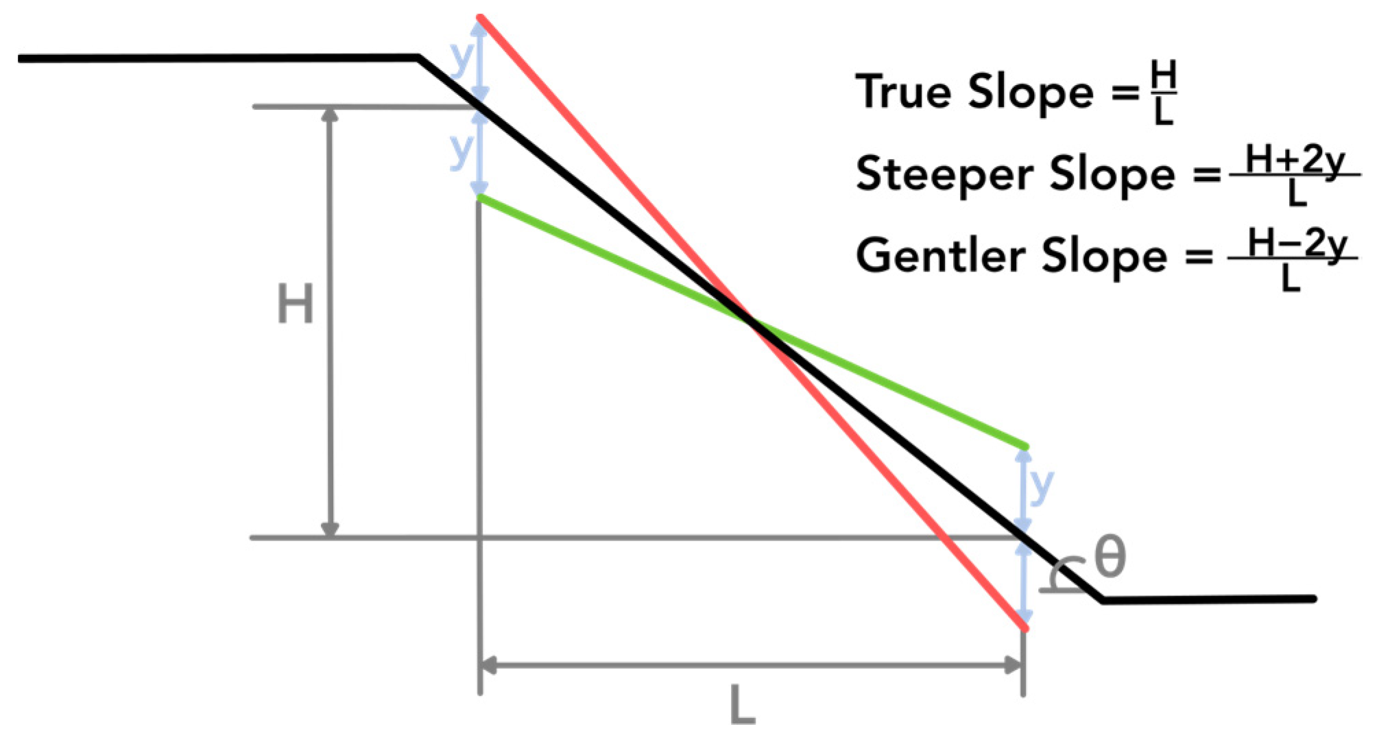
Studies have been completed based on 3DEP, formerly NED datasets which are now included in 3DEP, SRTM, ASTER, and AW3D30 databases with ground truth points to quantify accuracy [14,16,17,18]. The results of these accuracy studies are available in

Table 1. Reported vertical error of common open source DEMs available domestically in the United States and internationally. Vertical error is reported as the 95th percentile, calculated from RMSE when necessary. (NVA—non-vegetated area, VA—vegetated area).

DEM	3DEP NVA (1 m)	3DEP VA (1 m)	3DEP (2 m)	3DEP 5 m (Imagery)	NED April 2013 (10 m)	NED June 2003 (30 m)	AW3D30 (30 m)	SRTM (30 m)	ASTER ver. 2 (30 m)
95th Percentile Vertical Error (m)	0.196	0.3	0.392	2.7244	3.02	5.59	11.13	16.23	23.48
Reference	[16]	[16]	[14]	[14]	[17]	[17]	[18]	[18]	[18]

. Figure 2 illustrates the variability in these DEM systems for an example site outside of Yosemite National Park, California, USA. Though relative accuracy between two points is a potentially more direct method for computing slope angle error, widespread relative accuracy is seldom reported. The most commonly reported accuracy is RMSE, which is also the required reporting accuracy for DEM submittal for NED and 3DEP use, thus RMSE and converted absolute accuracy will be considered for comparison in this study, and simple trigonometry will be used to calculate potential slope angle error (Figure 3).

The application of vertical uncertainty for estimation of slope uncertainty as defined in Figure 1 and Equation (1) is most applicable in settings where the sliding surface is expected to be parallel to the slope surface (soil and regolith-controlled translational landslides, often shallower). This parallel assumption is used later in the study to investigate accumulated uncertainty, and the common occurrence of these surfaces paralleling one another is illustrated in the Results section. Most post-failure surfaces of landslides which may be under investigation today are covered by recent DEMs, but for accurate back-modeling, pre-failure topographies are often required. Previous studies, e.g., refs. [19,20] have noted a common alternative to the use of DEMs, when they are unavailable or resolution is unsuitable for analysis, or for constraining pre-failure topographies, is to mimic the topography of nearby slopes that do not have landslides. This approach, while offering some utility, presents significant challenges in accurately quantifying slope topography uncertainty, particularly when the original slope’s pre-failure condition is unknown. Moreover, the assumption that adjacent slopes with similar geological and hydrological conditions are equivalent may be flawed. The very differences in topography between the stable and failed slopes could be the critical factor that led to the failure. Beyond slope angle, slope topography may also control aspect-dependent weathering and microtopographic features that affect surface water ponding, further contributing to the instability, emphasizing that the failed slope’s distinct characteristics, rather than its similarities to neighboring slopes, may be the key to understanding the failure [21].

A more recent practice adapted for the consideration of pre-failure topographies is that of re-interpolation of the landslide polygon surface based on post-failure DEMs [22,23]. This practice involves the delineation of the landslide polygon on post-failure DEMs. From the polygon and the DEM, two surfaces can be created: one that has only the post-failure landslide surface, and nothing outside of it, and one that has the topographic surface excluding the landslide polygon. The pre-failure topography may then be interpolated within the landslide polygon through either direct raster interpolation into a DEM, or through the use of contour interpolation and subsequent conversion back to a DEM. Taking it a step further, the estimated pre-failure surface may also be clipped to the landslide polygon, and overlain with the post-failure surface to complete volumetric estimations. As with DEM resolution as a whole, the accuracy of this method is dependent on the relationship between the scale of the landslide and the resolution of the data to be interpolated, as well as the accuracy of the original post-failure DEM. A limited review does indicate, however, that interpolated pre-sliding surfaces do tend to exhibit the same general form as known original topographies, though they typically exhibit smoother contours [22]. In data-sparse settings, it could be argued that this is a more robust approach than simple slope mimicking, though due to smoothing effects, it may not be the most meaningful representation of landslide activities that are controlled by microtopographic features (such as terracing, levees, etc.).

2.1.2. Depth to Failure Plane

Depth to failure plane is a critical landslide parameter that determines the volume of material that may be mobilized, and in turn the portion of the driving forces defined by weight when calculating slope stability. Determining the depth of the failure plane requires defining a discrete two- or three-dimensional slip or shear surface where the failure, either partially or completely, is expected to occur.

Careful consideration of ground condition is critical for predicting the failure type and thus depth to failure plane of a landslide. Generally, more homogeneous materials, like unstratified soil or mass-weakened materials, exhibit rotational movement with circular failure planes, while stratification, structure, or other geologic inhomogeneity lend themselves to a translational failure along a plane of contrasting strength. Mass-weakened materials include those that have been deeply and homogenously weathered. Stepped rotational failure is common in areas of thinly stratified, weaker rockmasses where softening processes (i.e., slaking) may occur in susceptible layers, like shales. This simplified binning of landslide failure types must be considered alongside the complexities of anisotropy and structural control depth as related to the anticipated failure plane when selecting an analysis method based on landslide type. Many proposed calculation techniques are available in the literature for the estimation of failure plane depth, ranging from graphical extrapolations from the main scarp, e.g., refs. [24,25] to numerical modeling, e.g., refs. [24,26]. Ultimately, there is no shortage of mathematical approaches available, but the equations can be complicated and require many input values that are difficult to measure or estimate in data-sparse settings, further introducing uncertainty.

Typical simplified methods of slip surface definition outside of data-sparse settings include the use of boreholes, test pits, inclinometers, and geophysics. Even with data from these tools, the position of the slip surface may still be difficult to identify [27]. Translational landslides commonly occur at soil/regolith–bedrock contacts, or other geologic surfaces (faults, unit contacts, foliations, etc.) [24]. Therefore, one of the most powerful tools for estimating the depth to failure plane of a landslide may be the creation of a detailed geologic model of the site. In data-sparse settings, it is likely that this task will rely on existing geologic data. The confidence one may have in extrapolating them into the subsurface will likely vary from location to location, making the quantification of uncertainty challenging. Tools to verify or aid in the estimation of failure plane depths in data-sparse settings are summarized in

Table 2. Published methods for estimating the depth of landslide failure planes ordered from least to most complex/intensive, revised from [34]. R—Rotational, T—Translational, ()—potential or limited applicability.

Method	Landslide Type	Required Data	Description	Reference
Surface Area–Volume Relationship	R, T	🞄 Horizontal surface area or area along slope 🞄 Knowledge of expected geomorphic conditions (to apply correct power function from literature)	Defines failure plane by empirical power function and volume to depth conversion	[28]
Rheological Assumptions	T (R)	🞄 DEM 🞄 Rheologic interpretation 🞄 Displacement map	Defines failure plane by applying rheologic relations to surface velocity and depth	[29]
Surface Displacement Parallel to Slip Surface	R, T	🞄 Pre-failure surface 🞄 A series of displacement vectors	Defines failure plane based on parallel displacement to slip surface	[27]
Balanced Cross-section	T (R)	🞄 Longitudinal cross-section 🞄 Displacement along cross-section	Defines failure plane by assuming mass balance and calculating mass transfer	[30,31,32]
Volumes Controlled by Discontinuities	T	🞄 DEM 🞄 Structure orientations and locations	Defines failure plane by controlling failure surfaces	[33]
Half Ellipsoid or Elliptic Paraboloid	R	🞄 Landslide area 🞄 Maximum landslide depth	Defines failure plane with geometric shape	[24]
Empirical Transverse Cross-section	R (T)	🞄 Transverse cross-section(s) 🞄 Failure surface on lateral extents of landslide	Defines failure plane by empirical graphical relationship	[34]
3D Geomorphic Spline Calculation	R (T)	🞄 DEM 🞄 Failure surface on lateral extents of landslide	Defines failure plane using spline	[35,36]
Random Failure Surfaces and Probability	R, T	🞄 DEM 🞄 Discontinuity orientations 🞄 Discontinuity lengths and spacing	Defines failure plane by simulating stepped surfaces	[37]
Sloping Local Base Level (SLBL)	R (T)	🞄 DEM 🞄 Contours of initial failure surface	Defines failure plane by iterative calculation of quadratic failure surface	[38,39]
Depth Probability Calculations	R, T	🞄 DEM 🞄 Reliable estimate failure surface 🞄 Depth of hypothesized (deeper) failure surface	Defines probability of failure surface existing at a given depth	[28]

[24,27,28,29,30,31,32,33,34,35,36,37,38,39].

2.1.3. Depth to Water Table

In the absence of piezometer data, water table depth has classically been estimated using simple topographic controls, with estimated water tables typically appearing as a subdued replica of the land surface in cross-section [40], though instruction as to what degree the surface may be subdued is largely lacking in the available literature. Unlike estimations of slope topography, there have been few advances that would aid in the estimation of the water table surface using an off-site location as a surrogate.

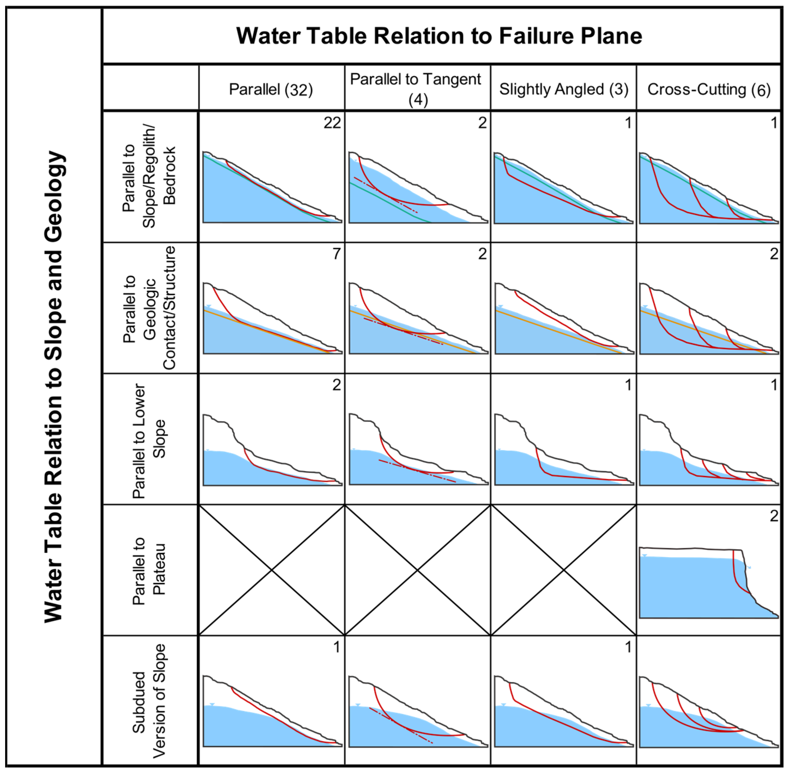
To inform water table estimations, we reviewed 27 translational landslide case studies and 9 rotational or hybrid landslide case studies to better define general water table trends in homogenous and inhomogeneous slopes. The results of this review are summarized in

Table 3. Summarized results of the literature review findings concerning water table estimation. Failure type, groundwater table characterization, instrumentation or data source, and groundwater table relation to failure plane are indicated (R—Rotational, T—Translational, # indicates an unreported number of a given investigation type).

Number	Failure Type	Groundwater Characterization						Groundwater Data Source		Groundwater Relation to Failure Plane				Reference
		Parallel to Smoothed Slope	Parallel to Regolith/Bedrock Boundary	Parallel to Geologic Contact	Parallel to Lower Slope	Parallel to Plateau	Subdued Version of Slope Topography	Piezometers/ Monitoring Wells	Boreholes/ Standpipe Wells	Parallel	Parallel to Tangent	Steeper/ Shallower	Cross-cutting or complex Landslide
1	R-T	x						2	24	x				[41]
2	T		x					6		x				[42]
3	R	x	x					4			x			[43]
4	R-T	x		x				9					x	[44]
5	R			x				4	1		x			[45]
6	T	x	x					4	4	x				[46]
7	T	x	x						21	x				[47]
8	T	x	x					9	7	x				[48]
9	T	x	x					10	25	x				[49]
10	T						x		9, and 22 shafts	x				[50,51]
11	T	x	x					2	2	x				[52]
12	T	x						3	2			x		[53]
13	R	x		x					5		x			[54]
14	R				x				3, and trenches		x			[55]
15	T	x		x					8	x				[56]
16	T			x	x			13	4	x				[57]
17	T		x		x				5	x				[58]
18	T	x	x						8	x				[59]
19	R-T	x						Back analysis		x				[60]
20	R-T		x			x		Remote sensing and regional wells					x	[61]
21	T	x	x	x					12	x				[62]
22	T	x		x					8	x				[63]
23	T	x						Back analysis		x				[64]
24	T				x			4				x		[65]
25	T	x						1	1	x				[66]
26	R					x		Remote sensing and regional wells					x	[67]
27	T	x	x					2	3	x				[68]
28	T	x	x					Regional controls		x				[69]
29	T			x				2	3	x				[70]
30	T	x	x						14	x				[71]
31	T	x	x					3	4	x				[72]
32	T	x		x				4	38	x				[73]
33	T			x	x			3					x	[74]
34	T	x	x						9	x				[75]
35	T						x		#			x		[76]
36	T	x		x				2	>40	x				[77]

[41,42,43,44,45,46,47,48,49,50,51,52,53,54,55,56,57,58,59,60,61,62,63,64,65,66,67,68,69,70,71,72,73,74,75,76,77].

From these case studies, it is evident that the water table rarely follows a subdued version of the original slope topography at the scale of an individual landslide (two of the 36 cases). In 29 of the 36 cases, the water table parallels the same feature that controls the landslide failure surface. In 24 of the 36 cases, the water table is approximately parallel to the slope. In 27 of the 36 cases, the water table was parallel to either a regolith or other geologic contact, with 18 of these 27 also parallel to the slope. Of the slides reviewed, these trends appear to occur independent of landslide scale and depth to failure plane.

When considering the two cases in which the water table was interpreted to be a subdued version of the slope topography (events 10 and 35 in Table 3), this typically occurs in homogenous settings, and on larger hillslopes and/or altered topographies (i.e., fill). This subdued surface is similar to the five cases in which the water table parallels the lower slope. Typically, this can be better described as the water table flattening to horizontal or sub-horizontal as the slope directly above steepens while approaching a crest, ridgeline, or alpine talus. Figure 4 demonstrates idealized examples of each of the reported water table conditions in relation to failure surfaces from Table 3 and may be used to inform water table estimation.

Table 4. Descriptions of observations potentially indicative of each reviewed water table geometry for use in water table estimation.

Water Table Relationship to Slope and Geology		Description Notes
	Parallel to Slope/Regolith/ Bedrock	Shallow to deep landslides in soil or regolith: - areas with well-developed vegetation - unconsolidated material - bedrock visible further upslope or above treeline
	Parallel to Geologic Contact/Structure	Moderate to deep landslides in weak rock: - vegetation may be sparse depending on rock type - bedding or other indications of in place rock, though may be decomposed - known regional bedding/structural orientation or known faults and shear zones - known hazardous units based on regional observations/history
	Parallel to Lower Slope	Shallow to moderate depth landslides in soil or decomposed rock: - variable slope at site, steepening with elevation - potentially the site of historic landslide - more vegetation and/or thicker soil mantle on the lower slope - common in large glacial or fluvial valleys with steep walls and flatter bank slopes
	Parallel to Plateau	Deep landslides through soil and bedrock at plateau or mesa margins: - vegetation and soil mantle on top of plateau, often irrigation as well - typically weak or weathered bedrock exposed on plateau sides - water table may be perched on bedrock, seepage at soil/rock contact common
	Subdued Version of Slope	Shallow to deep landslides in soil or regolith: - areas with more hydrophilic vegetation lower on the slope or other indicators of groundwater shallowing - scenarios in which the slope above a landslide would need to be considered (subduing visible on large scale, not on landslide scale itself)

summarizes field and geologic observations that may be indicative of a given water table condition.

Beyond water table shape considerations, and the use of visual cues to constrain depth, there are other tools that may aid in the refinement of estimations including the use of seeps and springs observed in estimations [78], infrared or thermal imaging [15], and ground penetrating radar (GPR) [79,80,81]. While discussed in more detail in Results, we note here that the thinner the soil mantle is, when analyzing translational slides, the more sensitive the slope will be to saturation and moisture changes [82]. Another consideration for the practitioner may be the presence of significant seepage forces in certain water table settings. These will need to be investigated and accounted for with site-specific data if they are desired to be considered.

2.1.4. Material Property Parameters

Before the stability of landslide material can be estimated, the nature of the material itself must be quantified, or in the absence of detailed data, must be estimated or assumed from regional geology, aerial imagery, or preliminary site investigation and mapping descriptions. A resource to identify shallow soils at a site is the NRCS Web Soil Survey (WSS), which gives soil units, descriptions, and United Soil Classification System (USCS) and American Association of State Highway and Transportation Officials (AASHTO) soil classifications over the majority of the United States. A similar international resource is SoilGrids1km, a global database of soil types and depth to bedrock on a 1 km grid scale. SoilGrids1km is reported to have a blanket accuracy of 23–52% [83], with limited description of how the accuracy of the platform was determined. Considering the large scale of SoilGrids, it is expected to have the most value when used with large landslides. When considering landslides outside of the United States, it may be one of the few surficial soil resources available.

A few general assumptions may also be implemented in the estimation of material property parameters: (1) assume there is no cohesion until proved otherwise [84,85,86], and (2) in undrained conditions concerning clays, friction angle can be assumed to be zero [87,88]. These are particularly useful assumptions when considering conservativism in forward modeling. It should be noted that using these conservative assumptions in back-modeling may result in inaccurate, or more uncertain water table and depth to failure plane estimates, as the non-uniqueness of back-modeling may result in compensation by one parameter to effectively make up for the poor estimation of another.

A commonly utilized source of material property estimations is literature values from either design standards or textbooks, e.g., refs. [89,90,91]. Though these textbooks are commonly referred to, a comprehensive listing of material parameters is yet to be compiled in literature. To address this need,

Table 5. Literature value ranges, compiled from multiple sources, for cohesion, friction angle, and unit weight of USCS soil types, mixtures, and specific descriptions. Continued on next page.

Category	USCS	Description	Cohesion (kPa)		Friction Angle (deg)		Unit Weight (kN/m3)		References
			Min	Max	Min	Max	Min	Max
Gravels	GW	Well graded gravel, sandy gravel, with little or no fines	0	0	33	40	20	22	[92,93,94,95]
	GP	Poorly graded gravel, sandy gravel, with little or no fines	0	0	32	44	19.5	21.5	[92,93,94]
	GW, GP	Sandy gravels	0	0	35	50	19	21	[96,97,98,99]
	GM	Silty gravels, silty sandy gravels	0	1	30	40	20.5	22.5	[92,100]
	GC	Clayey gravels, clayey sandy gravels	1	20	28	35	18	21	[92,100]
Sands	SW	Well graded sands, gravelly sands, with little or no fines	0	0	33	46	18.5	22.5	[89,92,93,94]
	SP	Poorly graded sands, gravelly sands, with little or no fines	0	0	27	39	17.5	21.5	[89,92,93,94,95,96]
	SM	Silty sands	20	50	27	35	18	23	[92,94,96]
	SC	Clayey sands	5	74	30	40	17	20	[92,94,96]
	SM, SC	Sand silt clay loam with slightly plastic fines	50	75	28	34	18	19	[93,94,98,101]
	SM, SC	Sand silt clay loam with slightly plastic fines (saturated)	10	20	28	34	--	--	[93,94,101]
	SW, SP	Sand	0	0	29	41	19	20	[92,93,98,102]
Silts	ML	Inorganic silts, silty or clayey fine sands, with slight plasticity	2	67	25	41	12	17	[89,92,94,96,100,103,104]
	MH	Inorganic silts of high plasticity	3	72	23	33	12	17	[92,94,100,104]
Clays	CL	Inorganic clays, silty clays, sandy clays of low plasticity	4	86	27	35	12.5	17	[92,94,96,100,104]
	CH	Inorganic clays of high plasticity	8	103	17	31	12.5	17	[92,94,96,100,104]
Organic Soils	OL	Inorganic clays of high plasticity	0	5	22	32	4	5	[92,104]
	OH	Organic clays of high plasticity	7	10	17	35	10	16	[92,100,103]
	Pt	Peat and other highly organic soils	10	21	0	10	8	14	[95,105,106]
Common Soil Mixtures	ML, OL, MH, OH	Silt loam	10	90	25	32	4	17	[93,94,103,104,105]
	ML, OL, CL, MH, CH	Clay loam, silty clay loam	10	105	18	32	4	17	[93,94,103,104]
	OL, CL, OH, CH	Silty clay	10	105	18	32	4	17	[93,94,100,103,104,105]
	CH, MH, OH, PT	High plastic silts and clays, organics	3	105	0	25	6	17	[94,100,101,103,104,105]
	ML, CL, OL	Silts, low plastic clays	3	105	25	30	12	17	[94,100,101,104]
	GW, GP, GM, GC, SW, SP	Sand, gravel, stone	0	0	32	48	15	21	[89,99,101]
	GW, SW, GC, GM	Mixture of gravel and sand with fines	1	3	15	28	18	22	[92,95,100,101]
	ML-CL	Mixture of inorganic silt and clay	22	65	25	41	15.5	19	[89,94,96,103]

and

Table 6. Literature value ranges, compiled from multiple sources, for cohesion and friction angle based on depositional environment rock type and material texture.

Category	USCS	Description	Cohesion (kPa)		Friction Angle (deg)		References
			Min	Max	Min	Max
Depositional Environment	GW, GP, GM	Alluvial-high energy	0		30	35	[95]
	ML, SM, SP, SW	Alluvial-low energy	0	24	15	30	[95]
	SP	Eolian-dune sand	0		30	35	[95]
	ML, SM	Eolian-loess	24	48	20	30	[95]
	SM, ML	Glacial-till	48	192	35	45	[95]
	GW, GP, SW, SP, SM	Glacial-outwash	0	48	30	40	[95]
	ML, SM, SP	Glacial-glaciolacustrine	0	144	15	35	[95]
	ML, SM, MH	Lacustrine-inorganic	0	10	5	20	[95]
	OL, PT	Lacustrine-organic	0	10	0	10	[95]
	SW, GW, SP	Marine-high energy	0		25	35	[95]
	ML, SM, MH	Marine-low energy	0	10	0	25	[95]
	ML, SM	Volcanic-tephra	0	48	20	35	[95]
	SM, SW, GM	Volcanic-lahar	0	48	25	40	[95]
Blasted/Broken Rock		Basalt	0		40	50	[97]
		Chalk	0		30	40	[97]
		Granite	0		45	50	[97]
		Limestone	0		35	40	[97]
		Sandstone	0		35	45	[97]
		Shale	0		30	35	[97]

were prepared to summarize literature values of cohesion, friction angle, and unit weight for several soil types and decomposed and broken rock [89,92,93,94,95,96,97,98,99,100,101,102,103,104,105,106]. The ranges given in these tables will also allow for the future analysis of anticipated uncertainty in a given parameter based on material and classification confidence.

From Table 5 and Table 6, it can be seen that clay and silt materials have the widest ranges of cohesion and unit weight values, and gravelly materials have the smallest ranges. In the complete absence of lab testing, or even field work, careful remote investigation and the use of literature values do appear to be reasonable means of estimating material parameters at the site of a landslide, though not without introducing uncertainty. Figure 5 and Figure 6 visualize the data presented in Table 5 and Table 6, respectively, in box and whisker plots.

Measurement of material strengths invariably requires assumptions of material homogeneity and consistent behavior over time. A complication in material strength property estimation is that many landslides occur in chemically and physically weakened rock, or rock with great potential to change either chemically or physically [107]. The occurrence of landslides in these weakened materials makes strength estimation challenging, as strength values may be highly variable over an engineering timescale. Despite the vast number of investigations completed into the strength and weakening processes of landslide-prone materials, very little guidance has been explicitly given for the estimation of primary material properties, though some approaches have been hypothesized [108,109]. Approaches including rockmass strength reduction based on the Geologic Strength Index (GSI) [110], have previously been used [111], though they do not always hold true in low-GSI materials, and they do not consider alterations in strength with saturation. It is recommended that initial ranges of material strength parameters based on literature be utilized, with the mean value of a parameter altered within the range during iterative back-analysis to reach a representative weakened value when no other data are available.

Given the resources available,

Table 7. Ranking of highest quality estimation practices for each critical parameter contingent unavailable data. Quality is defined as low, or reduced, uncertainty in estimation. Situational data availability may lead to estimation techniques not addressed in this table.

Estimation Guidance	Topography/DEM	Water Table	Material Parameters	Depth to Failure Surface
Highest Quality	3DEP 1 m	Incorporate known flow patterns, nearby well data, or other unique sources with field data to assess most likely water table geometry	Lab material classification/limited testing	Well constrained depth to bedrock data from available maps, nearby borings, web soil survey data
Intermediate Quality	3DEP 10 m	Use field observations to assess most likely water table geometry (with surface expressions of water)	Grain size distribution testing	Field observations of displacement and scarp development
	3DEP 30 m	Use field observations to assess most likely water table geometry (no surface expressions of water)	Mapping and field classification	Remote observations of displacement and scarp development
Lowest Quality	AW3D30 and SRTM 30 m	Remotely assess most likely water table geometry based on slope conditions and expected failure plane characteristics	Remote classification based on bedrock/expected weathering profile	Empirical relationships to investigate a slope with no evidence of prior motion

summarizes the most robust sources of estimation for each critical parameter given literature review results. The sources of uncertainty within each of these estimation techniques will be discussed in more detail in the following section.

2.2. Uncertainty Relationships

In order to best understand parameter uncertainty quantification through the lenses of sensitivity, amplification, and prioritization, uncertainty from each critical parameter was graphically visualized in a series of design charts. These design charts will aid in the prioritization of parameter investigation, and in the development of a framework for critical parameter estimation for data-sparse landslides, the Parameter Estimation Protocol (PEP).

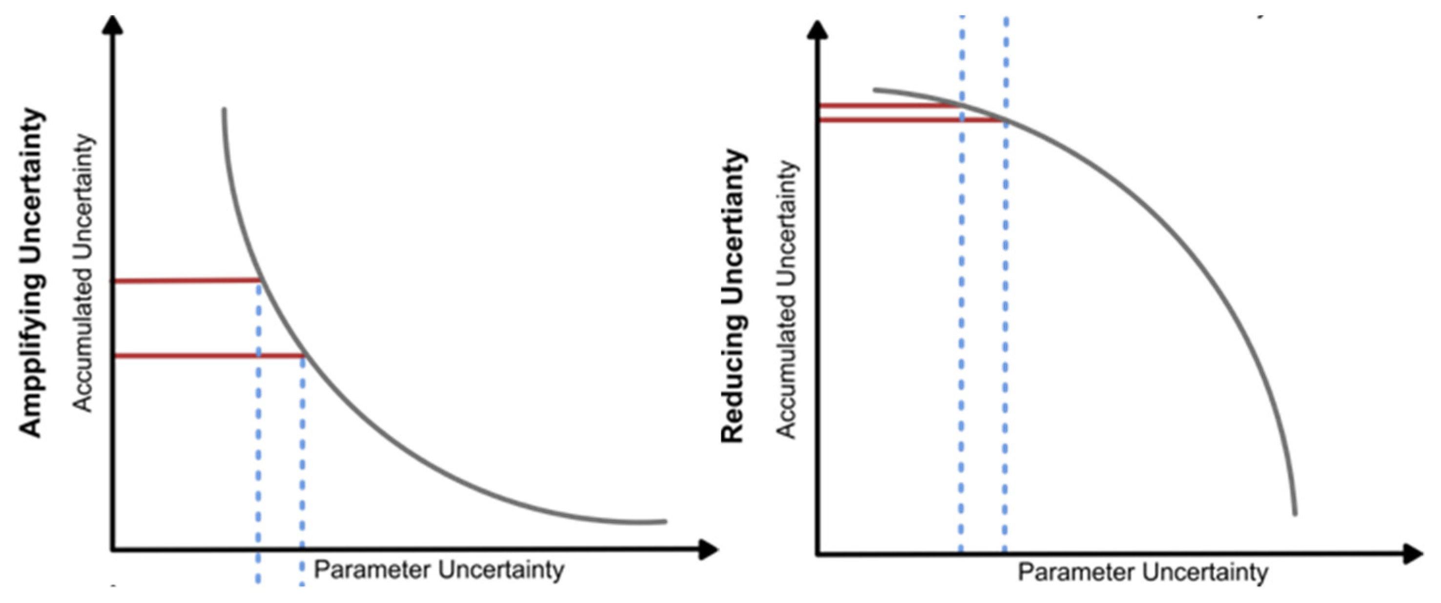
The following sections summarize the accumulated uncertainty (AU) in final slope stability calculations based on uncertainty in an individual parameter. Parameter uncertainty (PU) quantifies the range of likely values around some assumed or estimated mean value, expressed as either a percentage or absolute. Accumulated uncertainty is typically expressed as a percentage of the calculated factor of safety value, similar to percent difference calculations, and may be greater or less than PU depending on the amplifying or reducing relation between the two (Figure 7). Uncertainty definitions are summarized in

Table 8. A summary of the uncertainty types addressed in landslide analysis.

Uncertainty Type	Definition	Dependent Upon
Parameter Uncertainty (PU)	Uncertainty in a single parameter estimation	- Estimation technique - Data available - Range of potential parameter values
Accumulated Uncertainty (AU)	Uncertainty is FS calculation resultant from a given parameter uncertainty	- Parameter uncertainty - Landslide type - Landslide geometry/scale
Aggregate Uncertainty	Uncertainty in FS calculation resultant from interactions of all parameter uncertainties in a Monte-Carlo or similar analysis	- All parameter uncertainties - Compounding relationship of accumulated uncertainties - Landslide type - Landslide geometry/scale - Relationships between parameter uncertainties

.

Equation (2) demonstrates the calculation of uncertainties, as well as potential relationships between PU and AU.

$$\mathrm{A}\mathrm{U}={\displaystyle \frac{{FS}_u-{FS}_t}{{FS}_t}}\times 100$$

(2)

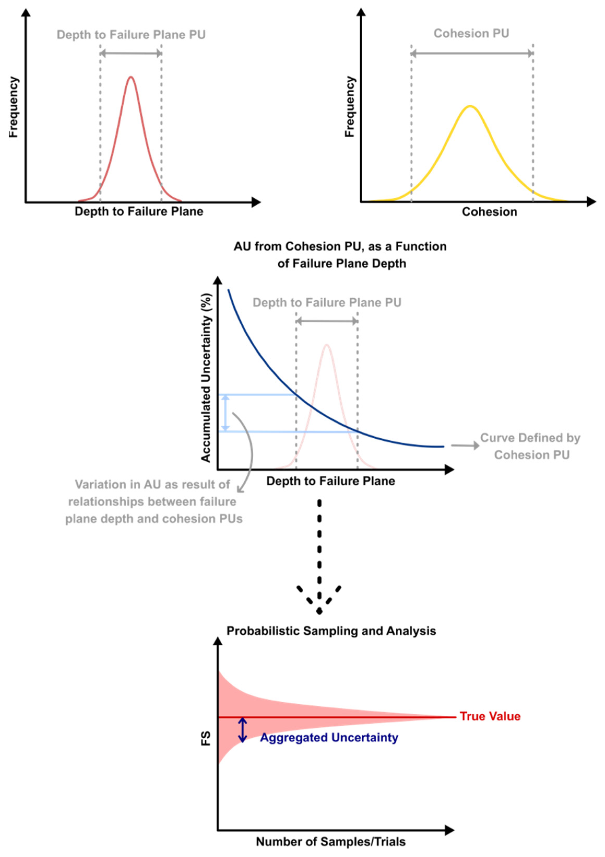
where ${FS}_t$ is the factor of safety calculated with the estimated parameter (theoretical) and ${FS}_u$ is the factor of safety calculated with a given parameter uncertainty (uncertain or experimental value). A third uncertainty term, aggregate uncertainty, may be defined as the resultant uncertainty in a slope stability analysis from all parameters, and considers all accumulated uncertainties. Aggregate uncertainty is dependent on the parameter magnitude and uncertainty magnitude of each estimated parameter, as well as slope geometry and scale, making it particularly challenging to quantify or to explain in terms of generalized trends, and reemphasizing the need for iterative analyses (i.e., Monte Carlo with multiple iterations of random sampling) (Figure 8).

To prepare uncertainty charts to help quantify and prioritize reduction in uncertainty, we use a simplified translational landslide model, analyzed for a large range of potential parameter uncertainties. In this model, we assume that the failure plane is roughly parallel to the angle of the slope surface. This is a commonly made assumption which relies on soil generation models [112,113,114,115,116]. This assumption allows for the simple geometric consideration of a single landslide thickness or depth to failure plane, as used in typical limit equilibrium calculations. Each set of analyses varies one parameter at a time. For the parameter(s) not being varied for a given analysis, fixed base values were used throughout each calculation (

Table 9. Fixed base parameters utilized as constants during the variation of the parameter and accumulated uncertainty calculations. In cohesionless cases, c = 0.

Parameter	Symbol	Value
Failure Plane Angle (deg)	q	30
Depth of Landslide (m)	z	10
Cohesion (kPa)	c	30
Friction Angle (deg)	f	40
Unit Weight (kN/m3)	g	18

).

2.2.1. Original Slope Topography

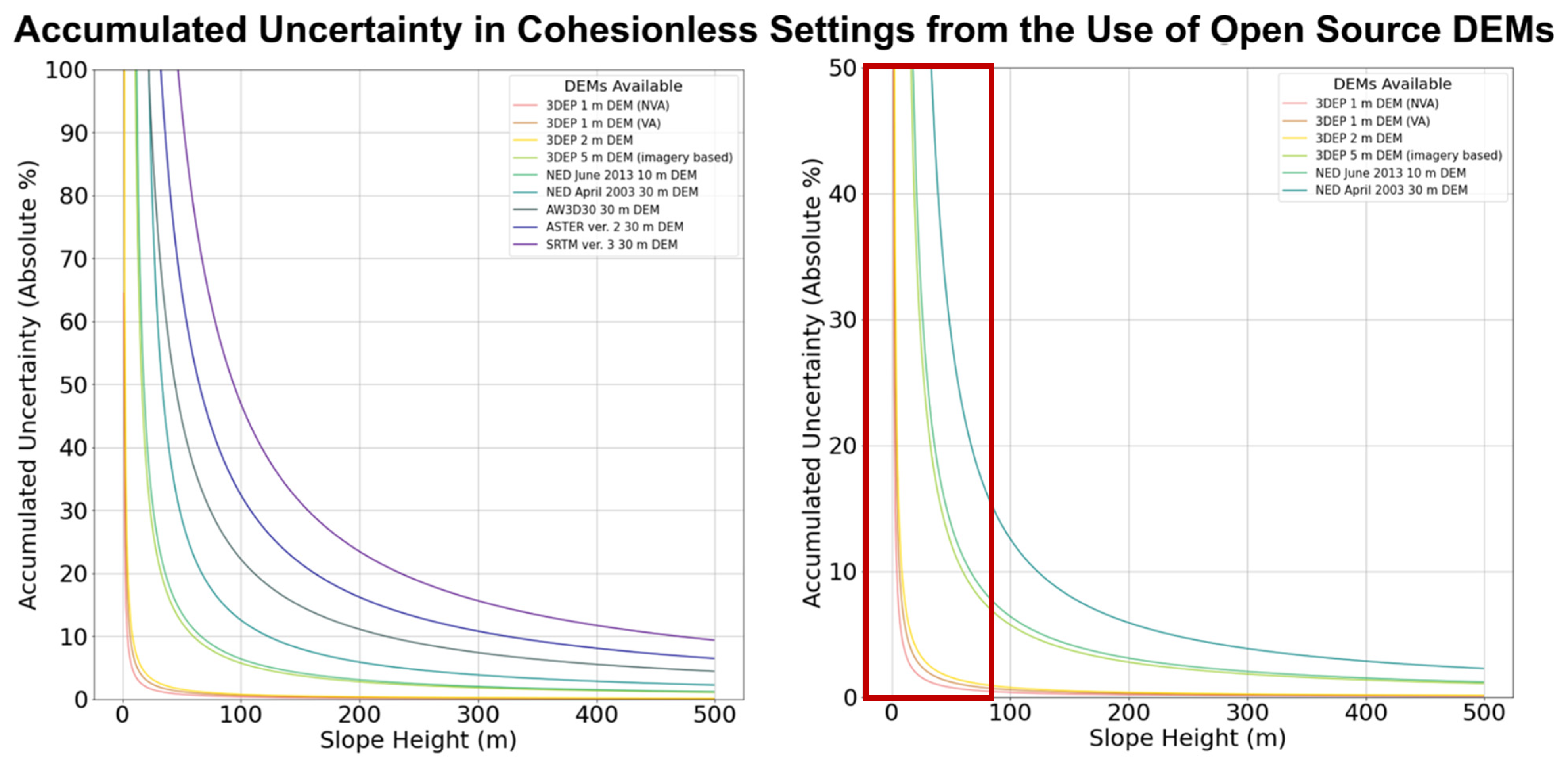
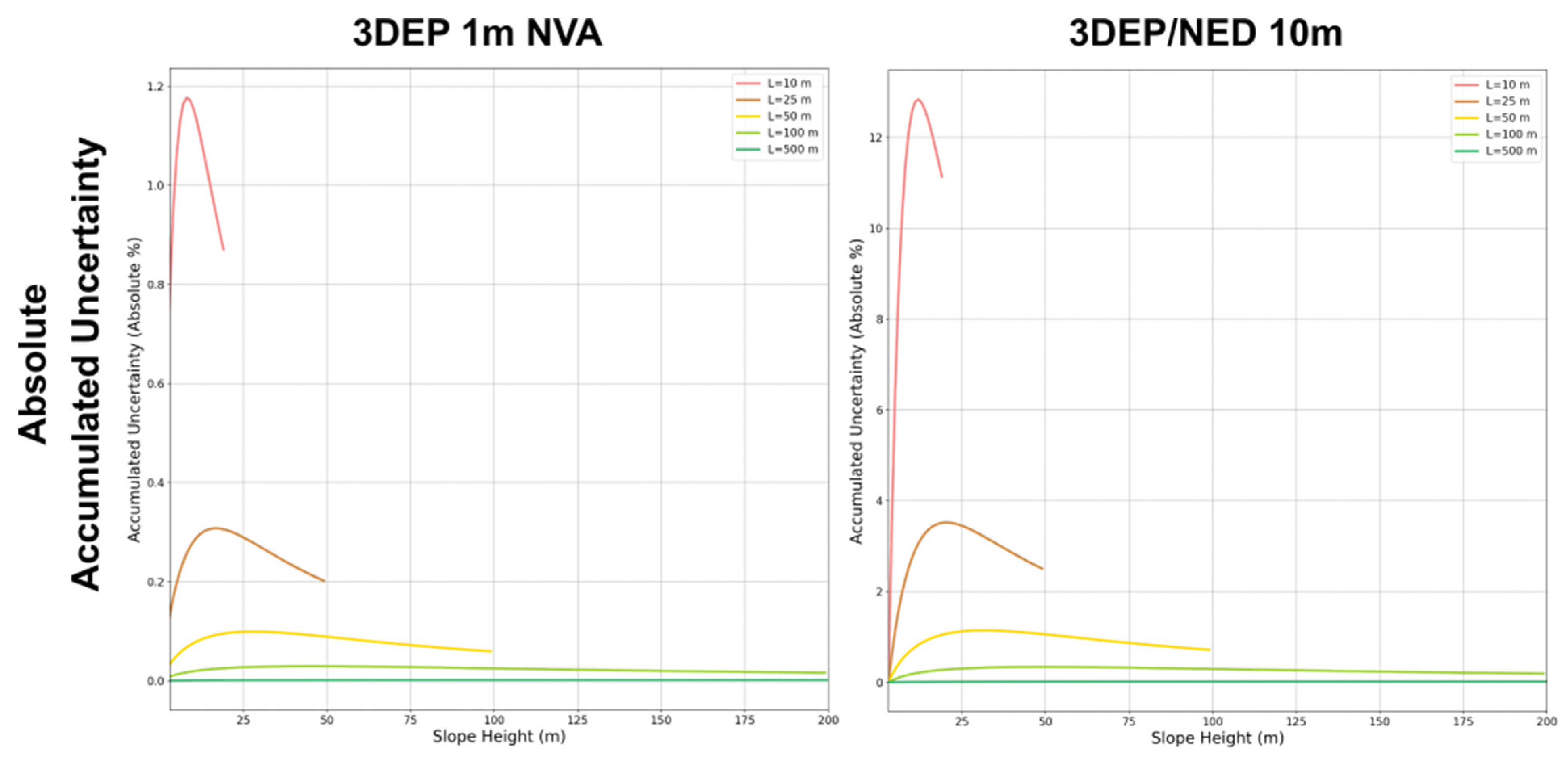
Using the vertical accuracy values reported in Table 1, and the calculations described, a series of design charts demonstrating the implications of failure slope angle uncertainty in factor of safety calculations as a function of slope geometries were developed (Figure 9 and Figure 10). These calculations were completed using the geometric relationships demonstrated in Figure 3, in which the maximum and minimum failure plane angles can be calculated from the vertical uncertainty reported for a given DEM. In Figure 9, for cohesionless settings, each curve corresponds to a different open-source DEM. The AU was calculated using Equation (2). The absolute value of the AU is plotted on the y axis, as a function of slope height, for each DEM reviewed. The theoretical factor of safety was calculated with the base values in Table 9, excluding the failure plane angle; and assuming zero uncertainty in the DEM. The factor of safety value calculated with parameter uncertainty, in this case, the vertical error in DEMs, was then calculated. Both factors of safety values were input into Equation (2) to calculate the percent change, or percent uncertainty in the final factor of safety calculations resulting from DEM vertical error. For settings with cohesion, AU becomes a function of both slope height and slope length. Thus, each design chart in Figure 10 is for a unique DEM, with the curves defined by landslide length, plotting AU as a percentage, as a function of slope height once again.

In cohesionless settings in Figure 9, the magnitude of AU asymptotically approaches zero as the height of the slope increases. The magnitude of AU from DEM use is dependent only on the DEM itself and slope height. When cohesion is considered in Figure 10, the magnitude of AU is dependent on the DEM uncertainty, as well as slope height, and slope length. The AU in settings with cohesion decreases as slope length increases, peaking at a height-to-length ratio (H/L Ratio) of approximately 1:2, and decreasing as slope height increases beyond the height-to-length ratio of 1:2. This peak behavior is the result of the FS calculation (Equation (1)) being defined by the trigonometry of the slope, namely the height-to-length ratio (slope angle). The AU peaks in settings with cohesion at the H/L ratio of 1:2 as a result of cohesion acting independently of all other terms which are scaled by the slope angle via trigonometric functions. This is representative of the physical understanding of soil slopes described by Equation (1), where cohesion is expected to have a lesser impact on stability at very low and very high slopes relative to other parameters. In cohesionless settings, there is no component of Equation (1) which is independent of height-to-length ratio, and thus asymptotic behavior is seen.

From these charts, based on landslide characteristics and the DEM used in the analysis, the maximum potential AU may be graphically estimated. The majority of the design charts indicate an inflection point where AU increases rapidly (Figure 9). This zone of variability can be described as a graphical area in which it is demonstrated that the slight alteration of one parameter (i.e., slope height for the example shown in Figure 9), may disproportionately increase the magnitude of AU from another parameter uncertainty (failure plane angle in Figure 9). These graphical zones therefore also demonstrate situations in which one parameter may be altered, re-estimated, or invested in (lab testing, instrumentation, etc.) to reduce not only its parameter uncertainty, but potentially the AU resultant from other parameters as well. The values at which these zones of inflection occur are summarized and presented in more detail in later sections.

Design charts similar to those presented in Figure 9 and Figure 10 were developed for the remaining parameters, as described in the following sections. All design charts are available in Supplemental Material S1. These design charts, grouped by landslide parameters, show the accumulated uncertainty in slope stability calculations resulting from different parameter uncertainties and the interaction of these parameter uncertainties with slope properties like depth of failure plane and height-to-length ratio. These charts may be used to triage the parameter(s) contributing the most to the uncertainty of a given slope stability calculation based on parameter estimation uncertainty and site characteristics, thus they may also be used to identify which parameters would be most cost-effective to invest resources to reduce uncertainty in final analyses. Accumulated uncertainty in the final calculation is generally presented in both general and absolute terms to aid in comparison.

2.2.2. Depth to Failure Plane

As discussed previously, there are many considerations when estimating the depth of the failure plane of a slide, all of which are based on available literature and remote data when working in data-sparse settings. As a result of these complications, the parameter uncertainty when considering depth to failure plane is best defined by engineering judgment on the part of the practitioner. As such, the parameter uncertainty described in design charts is given as a percentage. For example, an estimated depth to failure plane of 10 m with +/−0.5 m of uncertainty in absolute terms translates to 5% parameter uncertainty.

2.2.3. Depth to Water Table

Similar to the consideration of failure plane depth, guidance on shape and depth estimation may be provided. However, it remains challenging to provide guidance on the quantification of the uncertainty of this parameter. Data sources and geometries of water tables are exceedingly diverse, making it a highly variable parameter. With this in mind, it is considered that the quantification of water table location uncertainty will be considered with engineering judgment, informed by local knowledge, data availability, and confidence in interpretations. It should be noted that saturation and water table location also affect material property parameters in many situations. This poses a challenge to uncertainty quantification, and is discussed in more detail in the following section.

Differing from depth to failure plane, the parameter uncertainty in the design charts for saturated thickness is defined absolutely, as a magnitude in meters with a set percentage of the landslide body being saturated so that the thickness of the landslide and degree of saturation may be considered together. This approach was chosen as it may be more realistic to consider the water table as both a shape and depth which can be variable from point to point, as opposed to a fixed shape varying in depth expressed as a percentage. Though a single number for water table uncertainty still lacks nuance, it may allow for the estimator to more accurately describe the uncertainty as a meter magnitude instead of a percentage.

2.2.4. Material Property Parameters

In investigations where no direct sampling is possible, literature values of material strength are likely to be the only available resource for parameter estimation. Using the range of literature values for each soil type, a maximum uncertainty in each parameter may be defined. If possible, these ranges can be reduced with remote or limited field characterization.

Though many modeling software packages available today allow for the incorporation of material parameter uncertainties through a Monte Carlo-style analysis, the primary advancement proposed herein is the development of ready-to-use ranges of parameter values that may be used as inputs for these programs. The aim of the design charts in this section is to estimate the AU in final slope stability calculations and also to identify the parameters that control inflection points where AU increases rapidly.

Most landslides occur in clays and silts [107,108,117,118]. Unfortunately, clays and silts have the largest range of reasonable cohesion magnitudes when compared to other soils (Table 5 and Table 6). This lends many landslides to high cohesion parameter uncertainty. Design charts graphically visualizing the accumulation of cohesion parameter uncertainty are very similar to those previously presented; however, to aid in the visualization of data, some charts are presented in three dimensions.

Friction angle uncertainty ranges are smaller than those of cohesion (Table 5 and Table 6), limiting the maximum parameter uncertainty from estimation. Design charts graphically visualizing the accumulation of friction angle parameter uncertainty are very similar to those previously presented; as with cohesion, some of these relationships are visualized in three dimensions. Concerning both cohesion and friction angle, a negative correlation between these two strength parameters has been reported in previous studies [119,120,121,122]. Further investigation of its correlation would be needed to explicitly apply it to this work, but it remains a useful relationship to keep in mind during estimation, and should be used in conjunction with engineering judgment and available data when estimating parameters.

The range of unit weight values for non-lithified materials is smaller than that of either friction angle or cohesion, especially for soils, silts, and clays. This results in much smaller AU values compared to other material property parameters. Ranges of uncertainty for individual soils, soil types, and soil groups are summarized in Table 5 and Table 6. Design charts graphically visualizing the accumulation of unit weight parameter uncertainty are very similar to those previously presented; as with previous material property parameters.

2.2.5. Critical Fields of Rapidly Accumulating Uncertainty

As previously described and shown in design charts, the majority of parameter uncertainties result in accumulated uncertainties which indicate zones of rapid change in AU for a given parameter as a function of another. When estimated values fall within this zone, there is a potential to rapidly reduce or increase AU from a slight change in a secondary parameter uncertainty. In cases such as failure plane angle plotted as a function of slope height (Figure 9), in which slope height is not an estimated parameter, nor one which may be changed, the zone of rapid change is a region of consideration where As Low as Reasonably Possible (ALARP) methodology should be utilized [123,124,125]. Parameters that plot in this region should likely be considered for additional investment of time, testing, and investigation if the AU for the project exceeds the acceptable limit set by the user.

Table 10. Zones of inflection, or rapidly increasing accumulated uncertainty, for critical parameters, as well as summarized key trends in AU.

	Parameter	Approximate Landslide Thickness beyond Which AU Rapidly Increases (m)	AU Trends with H/L Ratio	Notes
Translational	Original Slope Topography	-	Peaks around H/L ratio ~1/2	🞄 AU rapid inflection in cohesionless settings:
				For DEM resolution < 5 m: slope height < 25 m
				For DEM resolution > 5 m: slope height < 100 m
	Depth to Water Table	<10 [for PU <2 m]	Decreases as H/L ratio increases	🞄 When <50% of slide thickness is saturated, AU increases for a given PU
		<30 [for PU >2 m]
	Depth to Failure Plane	<10	Increases as H/L ratio increases	🞄 Underestimations affect absolute AU more than overestimations
	Cohesion	<20	Increases as H/L ratio increases	🞄 Magnitude of cohesion has minimal impact on AU
	Friction Angle	>10 [AU levels off high]	Decreases as H/L ratio increases	🞄 Overestimations affect absolute AU more than underestimations; magnitudes >40 degrees rapidly increase AU
		<10 [AU rapidly decreases]
	Unit Weight	<15	Increases as H/L ratio increases	🞄 Underestimations affect absolute AU more than overestimations; magnitude has minimal impact below 50% PU

summarizes these zones of inflection for each critical parameter as well as additional notes on AU trends.

From Table 10 (and Supplemental Material S1), two additional observations can help manage uncertainty when analyzing data-sparse landslide analysis. First, shallower landslides typically accumulate uncertainty more rapidly than larger landslides. That is, larger landslides are less affected by uncertainty ranges because the uncertainty is averaged out over a larger distance. Second, for translational landslides, AU typically increases with increasing height-to-length ratio. This follows a similar intuitive idea: smaller, steeper landslides are more sensitive to uncertainty in input values than longer and/or deeper landslides.

3. Results

Following the interpretation of data presented in the prior sections, a general workflow was developed for the analysis of data-sparse landslides, including means of estimating parameter magnitude and uncertainty as well as AU. This workflow, the parameter estimation protocol (PEP), is available in its entirety in Supplemental Material S2. The comprehensive landslide workflow guided the development of a summarized workflow that focuses on parameter estimation and uncertainty reduction (Figure 11) with additional guidance summarizing the most likely sources of AU for given landslide conditions presented in

Table 11. Generalized landslide divisions based on failure plane type, maximum depth, and height-to-length ratio used in analysis with corresponding parameters that accumulate the most uncertainty for a given condition, listed in order of decreasing contribution to accumulated uncertainty.

Maximum Depth	H/L Ratio	Typical Parameters with Greatest Uncertainty Accumulation
Shallow	<1/2	Water Table, Friction Angle, Failure Plane Depth
	>1/2	Water Table, Failure Plane Depth
Medium	<1/2	Water Table, Friction Angle, Failure Plane Depth
	>1/2	Water Table, Failure Plane Depth
Deep	<1/2	Water Table, Friction Angle
	>1/2	Water Table, Friction Angle, Unit Weight, Failure Plane Depth

. The PEP is most applicable for use at soil/regolith-mantled translational landslides, and is limited in applicability to rock-slide type hazards.

The columns of the flowchart in Figure 11 are organized by analysis parameters and/or modeling procedure. The first four columns, which are labeled by parameter, include methods for estimation, most of which are intended to be used within back-analysis. The final column, labeled Uncertainty Quantification describes modeling goals and refers to uncertainty guidance within this work. In the complete workflow within Supplemental Material S2, the figure is further divided into three rows. The upper row illustrates the general steps of analysis, in the recommended order for initial estimations and analysis—before estimations are narrowed and a factor of safety near one is reached for back-modeling. The second, or middle, row describes estimation criteria and refers to tools in previous sections that may be used to inform analysis. The lower row describes common sources of uncertainty for each critical parameter, and references resources within this study that may be used to quantify uncertainty values and prioritize resources for further detailed analysis.

The initial process of analysis entails the collection and preparation of open-source data required to define the landslide model along (nominally) four cross-sections roughly parallel to the vector of motion of the landslide. Parameter values within this framework are then estimated based on the data available. Following the first iteration, parameters should be re-estimated based on the results of the first computation in order to decrease the impact on AU. The parameter expected to have the greatest influence on AU should be narrowed within the anticipated literature ranges first. It is recommended that re-estimation for back analysis is completed in a halving approach (explained below), stepping out as needed. The use of design charts, as shown in the previous section can allow for the identification of these parameters for a given landslide condition. The order in which parameters may be reasonably re-assessed to reduce AU, on the basis of landslide type and failure surface depth, is summarized in Table 11.

As the computed factor of safety for a given cross-section nears unity, the sensitivity analyses may be used to identify which parameter(s) is most impactful to the factor of safety based on the estimated ranges. The workflow is then completed on the remaining cross-sections to provide a sort of internal calibration. The parameter value results of all four cross-sections may then be used to further narrow the ranges of each parameter in each section based on evidence of limiting magnitude in another section.

The halving approach, demonstrated in Figure 12, aims to reduce estimation time and number of trials when narrowing on a range of reasonable values. This approach uses the following steps:

• Begin with the full range of material properties values based on data available
• Based on initial computational results, halve the length of the initial range, centered on a preferred estimated value from either literature or other available data at the site
• Based on computational results, repeat Step 2 based on engineering judgment and results of sensitivity analyses in back modeling (i.e., halve the range again if the results of Step 2 return tails far beyond FS = 1 when back modeling)
• If the range of a prior step is too narrow (does not reasonably span the values which result in an FS near 1) expand the range along the same center by fifty percent (twenty-five percent in either direction) to capture more likely values
• If it is desired, to slightly narrow the range of a prior step, final adjustments on either end of the distribution should be made.

Intermediate to these steps the value on which the range is centered may be moved while maintaining the range of the prior step to a newly hypothesized value. This approach should be supplemented with data as available from observations, lab tests, or detailed local material literature values to more efficiently inform estimation and the narrowing of likely values.

Completing this iterative process while focusing on the most sensitive landslide parameters greatly increases the efficiency of back-modeling analysis. Forward analysis then requires the use of post-failure DEMs and the estimated depth to failure surface/geologic contact and depth to water table based on the observations made during back-modeling. While it may introduce more uncertainty in the calculation, it may be appropriate to use the estimated residual strength of the landslide mass after sliding when there is a field or other evidence for significant weakening of material for more conservative forward modeling.

3.1. Efficacy and Example

3.1.1. Test Site

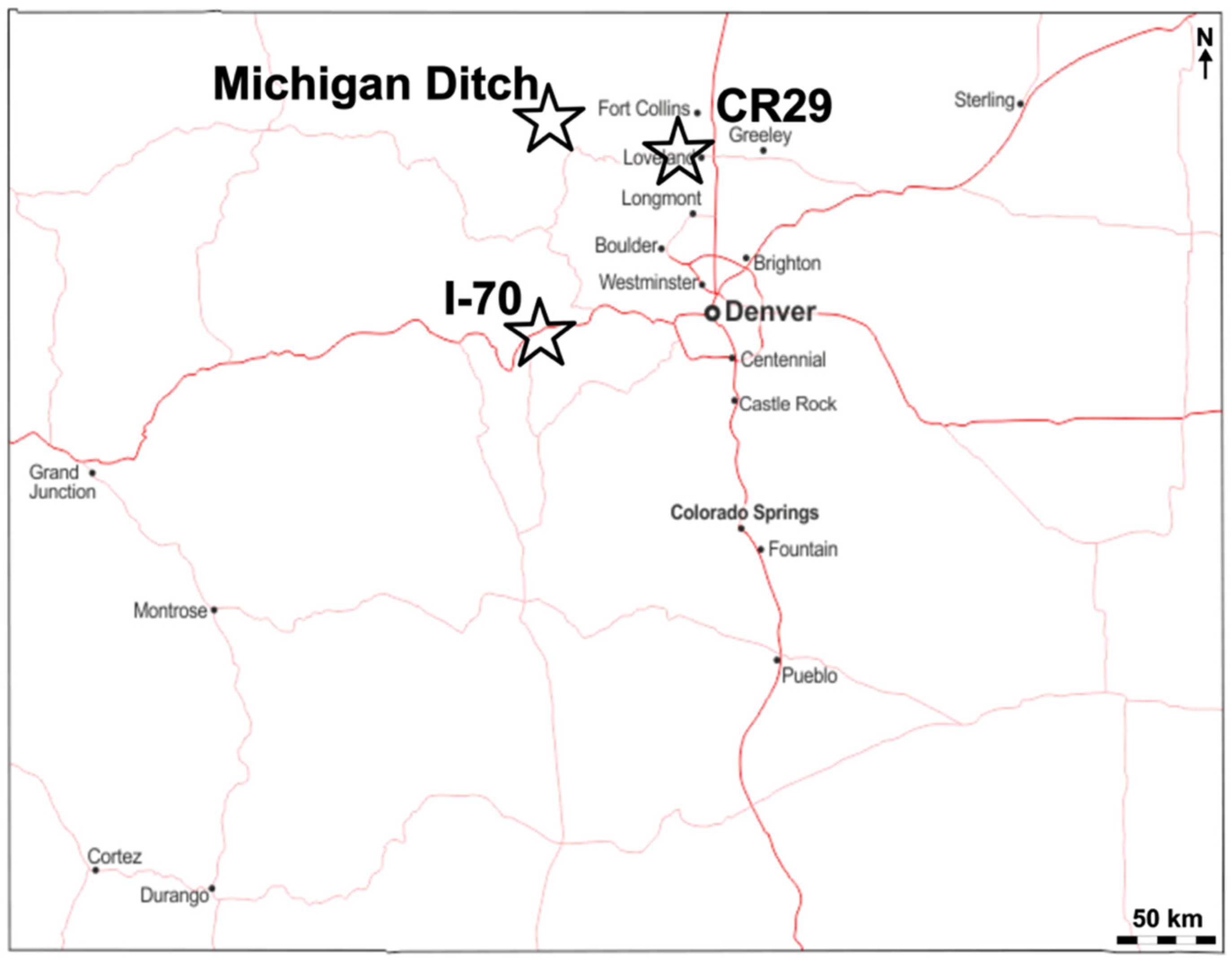
To verify the efficacy of the proposed PEP model for data-sparse landslide analysis, the proposed workflow was applied to three landslides in Colorado: the Michigan Ditch landslide, the I-70 landslide west of Eisenhower Tunnel, and the County Road 29 landslide west of Loveland, CO (Figure 13). These landslides were selected based on their range of sizes and anticipated characteristics that would allow for the PEP model to be applied across a broad range of settings. Each of these landslides has been previously investigated in varying levels of detail, and thus have pre-existing lab testing and/or field instrumentation (LT/FI) models. For this study, each landslide was analyzed as if there were no data available, without viewing the published investigation results. Following analysis, the results using the data-sparse methodology from this study were compared to the results of LT/FI models to judge the performance of the data-sparse analysis for the general characterization of the landslide. In this work, the Michigan Ditch landslide will be discussed in detail: all three cases are available for review [126].

The Michigan Ditch landslide is located above Cameron Pass, near the Continental Divide in northern Colorado (Figure 13). The landslide, while not the only landslide along the Michigan Ditch (a water conveyance canal), has previously been one of the largest and most destructive in the right-of-way. In 2015, the landslide had activated and displaced to such a degree that the ditch was covered, and water flow was halted.

3.1.2. Available Data

For the data-sparse analysis of the landslide, there was limited open-source data available due to the remote location of the landslide. Geologic data publicly available related to the landslide were limited to quadrangle-scale and larger regional geologic maps. From the most detailed map available, at 1:50,000 scale [127], the area was mapped as a landslide deposit. The presence of this landslide on a geologic map pre-dating widespread open-source DEM availability indicates that no pre-failure DEMs are available for analysis. Though the map did not provide details on the materials at the site, the surrounding geology was used to aid in the interpretation of field mapping. The landslide is located in a structurally and materially complex corridor, with tertiary ashes and tuffs, Precambrian metamorphics, as well as more competent Tertiary volcanics and intrusions in a heavily faulted and sheared area striking roughly parallel to the fall line of the landslide. Evidence of this faulting and rubbilization was verified during field mapping and site reconnaissance. The composition of the Precambrian and ash/tuff units on and above the landslide slope are prone to weathering and decomposition, particularly when in a shear zone, creating a thicker soil mantle at the site.

For the consideration of original slope topography, multiple SRTM DEMs were available at variable resolution, including AWD30 and NED 10 m and 30 m DEMs (note: the NED program has been discontinued and incorporated into 3DEP at lower resolution; these are the same data as in the NED DEMs). There were also a small number of other open source DEMs available, mostly on the international scale, at 30 m raster resolution or below. As is apparent from this list, there was no 3DEP 1 m availability at this location. The 10 m NED DEM was selected for the analysis of this landslide as the highest resolution and best-reported vertical accuracy of those available [128]. There was no DEM available which pre-dated the failure at the landslide, and thus pre-failure topographies were interpolated for the analysis.

Other data available for this location include satellite imagery available on GoogleEarth and PlanetLabs to visualize groundwater changes over time, as well as NRCS WSS data which cover a portion of the area with limited data and soil characterization.

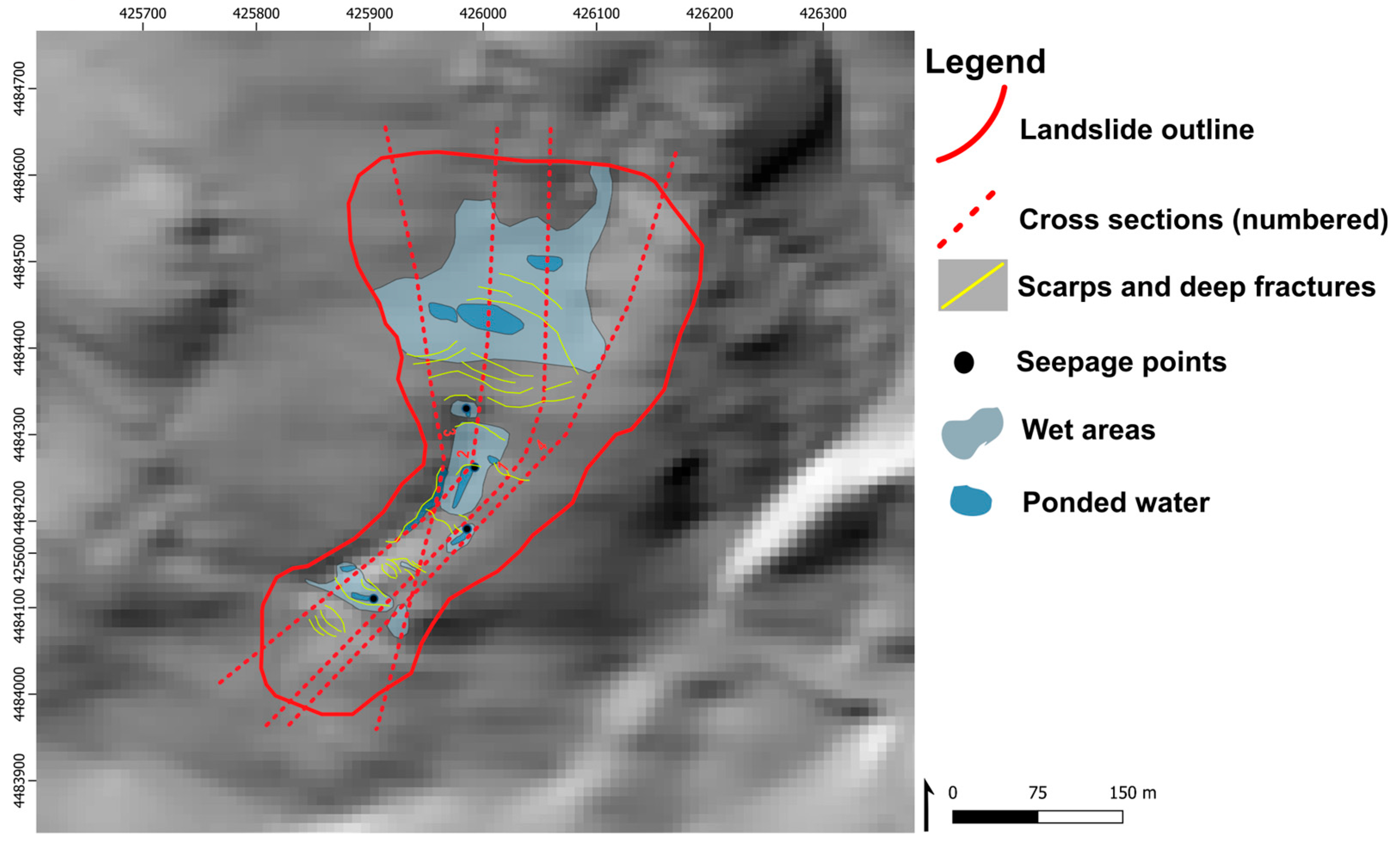
Following an initial desktop study which included the preliminary delineation of the active landslide, ponded water, and review of the geologic background, field work was completed at the site on 1 October 2022. To simulate a true data-sparse analysis, no samples were collected, and no lab tests were performed. The primary goals of the fieldwork were to map the landslide as if nothing was known about the site structurally, hydrologically, and regarding site materials (Figure 14).

The structural map produced indicates the complexity of the landslide, with multiple scarps and scarp zones creating intense and numerous hummocks along the slope. Ground fissures and vertical offset were observed at the lateral limits of the slide mass, particularly on the western lateral margin (Figure 14).

Qualitatively, numerous curved tree trunks indicative of downslope motion were observed in both young and old trees. The surface material seen during field work was relatively similar across the landslide body, with the exception of imported fill near, and covering, the access road and ditch across the toe of the landslide. The flattened area near the headscarp, surrounding the large ponded water pools at the treeline, was noted to include less coarse material (coarse sands to gravels) than the colluvium within the main slide body. The material did not appear or feel different enough in the field to be separately classified, particularly without lab analyses or other supporting evidence for the division. The most notable qualitative observation made at the landslide was the saturation of the soil and the presence of seeps at every large scarp face, usually approximately 1 m from the top of the scarp surface. Across the main body of the landslide, shallow water pooled on the surface between small hummocks. There had been no precipitation at the landslide, or upstream of it, for over a week before the site visit, with the exception of a frost coating deposited the evening before field work. It is unclear if this was freezing of water already at the site, or a dusting of snow in the evening. It is not expected that this small amount of moisture would lead to saturation and seepage seen at the site, particularly when the longstanding ponded water at the head of the landslide is considered. The application of the PEP model to this landslide incorporated these considerations.

3.1.3. Application of the PEP Model

Before the application of the PEP model began, a list of considerations based on location and known data were compiled. These are summarized below in

Table 12. Considerations for parameter estimation and at the Michigan Ditch landslide sorted by parameter.

Parameter	Considerations
Topography	Highest resolution DEM available is NED 10 m No pre-failure DEM topography available
Depth to Water Table	Frost activity expected due to elevation and location (seasonal) Ponding water, springs, and surface saturation indicative of shallow water table
Material Parameters	Surficial material initially classified as SP/ML in the field, with some areas having a more significant gravel component Regolith and weathered rock expected beneath soil Bedrock regionally mapped as igneous.
Depth to Failure Plane	Regional geology indicates crystalline bedrock below quaternary deposits, limiting failure plane depth and water table Quaternary deposits and forested location indicate translational failure

.

To begin, a preliminary geologic model based on available data and field observations was developed. With this preliminary model in mind, the workflow for interpolating pre-failure surfaces based on post-failure DEMs was implemented. Using the interpolated DEM, four cross-sections were generated roughly parallel to the local direction of landslide motion. These cross-sections are not parallel to one another, and some are not along the same cardinal direction for the duration of the line due to anticipated changes in fall line direction with topography. The initial geologic model was then applied to each of the cross-sections, with care taken to maintain average soil thickness and bedrock elevation across all cross-sections.

The geologic model of the landslide included three basic units: surficial soil cover mapped and described during field work, a weak/weathered regolith layer, and bedrock. Evidence of the presence of the weak regolith layer included angular, fractured rhyolitic clasts increasing in number with depth (1.5 m) visible in the faces of vertical scarps; fragments of weathered rhyolitic bedrock (cobble to gravel-sized) in the roots of felled trees; and the known local shearing, interpreted to increase fracture density and accelerate weathering of the regolith. The contacts between the soil/regolith/bedrock units were drawn approximately parallel to the slope based on typical regolith and soil development. The majority of the uncertainty in this geologic interpretation and model is related to the degree of faulting and fault-related deformation and groundwater flow alteration creating secondary permeability/porosity. Though the topography is indicative of the mapped upslope fault, soil cover and vegetation masked potential evidence to characterize the extent of the deformation zone. Due to the lack of evidence, and potential variation introduced with a poorly constrained shear zone interpretation, the simpler soil horizon-based model was maintained for analysis.

These cross-sections were built and recorded in RocScience’s Slide2 software Version 11.017. Slide2 is a two-dimensional slope stability analysis software designed to evaluate the safety of natural and engineering slopes. It uses the limit equilibrium method to analyze the stability of a single two-dimensional cross-section of a landslide at a time. Slide2 may be operated solely with the critical data-sparse parameters in this study, or additional complexities may be added in the case that data are sufficient to justify. For application with the PEP, it is recommended that Slide2 or a similar software be used, as these programs allow for the incorporation of probabilistic analysis, while minimizing the number of user inputs which may increase uncertainty.

Following the development of the four geologic cross-sections, water tables were initially estimated using Figure 4 and Table 4. Field and satellite observations, as well as the geologic model, indicate that the simple slope parallel water table assumption is the most applicable, and requires the fewest assumptions about the site. The water table was initially incorporated into the model probabilistically, honoring the uncertainty in-depth and allowing for initial sensitivity analyses. To do this, a maximum and minimum probable water table was drawn, with the median water table between the two calculated by the computer stability program Slide2. The minimum water table was initially estimated to be at the soil regolith contact, and based on field observations, the maximum water table was placed about 0.25 m beneath the ground surface parallel to both the slope and the minimum water table surface.

Material properties were then selected for each material, based on literature values, field observations, and bedrock maps. The initial values selected were the medians of literature ranges. As this step was also completed probabilistically, ranges for each of the three material property parameters were selected using the literature range minimums and maximums in Table 5, as no other outside data or sampling were available to reduce uncertainty.

Based on the geologic model developed for the site, and the interpretation of the landslide as translational, it was expected that the regolith layer controlled the failure surface of the landslide. As the regolith layer location was previously constrained within reason based on the geologic data available, the modeled failure plane, as iteratively calculated by Slide2, was validated against the regolith location. To prepare for computation, the entire model was set as probabilistic, with a Latin hypercube sampling method, and 1000 samples. The distribution of material property parameters as well as water table depth was set as normal. Finally, the failure surface was defined to be non-circular, allowing the predicted translational failure to be modeled.

Following the initial run of the model, the factor of safety of the weakest analyzed failure surface, the location of the surface, and the sensitivity analysis output by the initial model were reviewed for convergence with expected failure surfaces and a factor of safety of unity.

The initial results indicated a curved, dipping failure surface, deepening with distance down the slope. There was no evidence from the field to support the more hybrid-style landslide initially modeled, nor the depth of failure plane produced by the preliminary results. It was interpreted from these results that the material parameters of the soil and regolith used were much stronger than what is likely present at the site. Specifically, the assumed parameters overestimated cohesion, preventing the modeled failure surface from occurring along the regolith boundary as hypothesized. The cohesion value for the soil was modified from the median literature value utilizing a stepping-out approach to narrow the range of probable values. Ultimately a cohesion value of 2 kPa, with the minimum value set at 0 kPa, and the maximum at 4 kPa was reached.

Though the second iteration of back-modeling resulted in more realistic failure surfaces and factors of safety, there was still a need to reduce the factor of safety to satisfy the near-unity requirement of back-modeling. The results of the sensitivity analysis were analyzed with consideration of field observations and the interpreted geologic framework. The water table location and friction angle magnitudes of the soil and regolith material were the parameters identified as most impactful on the factor of safety. The range of water table depths considered to this point was nearly 12 m, ranging from 0.25 m beneath the ground surface to nearly 12 m. The saturated conditions on site, as well as ponded water and dense vegetation visible over decades of aerial imagery, suggest that the water table surface is likely not as deep as 12 m. Therefore, the maximum depth of the water table was altered to be approximately 8 m beneath the ground surface, maintaining the slope-parallel orientation which was initially modeled. The final parameter estimations are summarized in

Table 13. Final material property parameters used for the analysis of the Michigan Ditch “Mudslide” landslide. Minimum and maximum values are set based on narrowing of probable values from the initial literature range based on results, and serve as limits for sensitivity analysis calculations.

	Cohesion (kPa)			Friction Angle (deg)			Unit Weight (kN/m3)
	Mean	Min.	Max.	Mean	Min.	Max.	Mean	Min.	Max.
Soil	2	0	4	25	17	33	20	17.5	23
Regolith	0	0	0.5	35	30	40	20	18	22
Bedrock	32,300	27,750	36,850	55	53.2	56.8	21	20	22

; as refined using the halving and stepping-out approach presented in Figure 12.

The most likely plane of failure in three of the four cross-sections is a translational plane roughly coincident with the regolith–soil contact, as hypothesized after field analysis. The single failure plane that did not align with the regolith contact exhibited a lower dip and more rotational characteristics than the other sections, with an anomalously high calculated factor of safety compared to the other sections. It is anticipated that not all sections will yield the same results, due to unincorporated factors such as three-dimensional effects and side friction. It should also be noted that, as seen in Figure 14, this section is less parallel to the anticipated direction of movement of the landslide than the others. The final material property parameters are within the literature ranges of the materials observed on the slope, and honor the data collected while mapping.

3.1.4. Agreement with the LT/FI Model Findings

To validate the proposed workflow, the estimated results, parameter estimations, and parameter uncertainty were compared to the LT/FI model results.

Table 14. Reported values from the LT/FI analysis, parameter uncertainty, as a percentage, for each parameter estimation, and percent change in mean parameters estimated in the PEP workflow from those reported in the LT/FI analysis at Michigan Ditch [129].

		Cohesion (kPa)	Friction Angle (deg)	Unit Weight (kN/m3)	Depth to Failure Plane (m)	Depth to Water Table (m)
Reported Value	Soil	0	25	18.85	11	4
	Regolith	0	32	19.632
	Bedrock	0	42	23.563
		Cohesion	Friction Angle	Unit Weight	Depth to Failure Plane	Depth to Water Table	Depth to Bedrock
Parameter Uncertainty (+/−%)	Soil	50.0	24.2	13.0	70.0	50.0	40.0
	Regolith	50.0	12.5	9.1
	Bedrock	12.3	3.2	4.5
Deviation from LT/FI Analysis (% error)	Soil	--	0.0	6.1	18.2	0.0	18.2
	Regolith	0.0	9.4	3.3
	Bedrock	--	30.1	6.6

summarizes the data previously collected at the landslide [129].

When the LT/FI model is compared to the PEP model presented in Table 13, the overall geologic model and geometry interpreted at the site are quantitatively very similar [129]. Quantitatively, Table 14 illustrates which parameter estimations had the largest deviations from the LT/FI model, and if these deviations were anticipated based on the uncertainty assigned to the estimation initially. Parameter uncertainty for all parameters is expressed as a percentage, calculated as the change from the mean to the minimum or maximum value of the parameter. The deviation from LT/FI model results is also expressed as a percent change from the mean estimated parameter to the mean reported value. For most parameters, there was only one reported value.

From Table 14 it can be seen that of the three material property parameters considered, the parameter with the largest estimation uncertainty, cohesion, also deviated the furthest from the LT/FI model [129]. In large part, this is the result of the data-sparse model having minimal soil cohesion (<3 kPa) and the bedrock using literature values of 32,300 kPa for igneous crystalline rock, while the LT/FI model assumed zero cohesion for both of these units [129].

The greatest parameter uncertainties were in-depth estimations, likely the result of over-conservatism on the part of the estimator. Using the proposed water table estimation techniques supplemented by field observations, the median water table was finalized at 4 m, with an upper limit of just below the surface, and a lower limit of 8 m. The LT/FI model water table in borings on site was 4 m [129]. Though there was large parameter uncertainty in this estimation, it did prove to be representative of the site. Similarly, considering depth to failure plane and depth to bedrock/geologic estimations, the parameter uncertainty was much larger in magnitude than the deviation from the LT/FI model.

A summary of the maximum predicted AU resultant from each parameter is in

Table 15. The predicted AU from each PU at the Michigan Ditch landslide.

		Cohesion	Friction Angle	Unit Weight	Depth to Failure Plane	Depth to Water Table	DEM
Accumulated Uncertainty (+/−%)	Soil	15	20	1	30	25	<0.01
	Regolith	15	20	1
	Bedrock	4	2	0.5

. To develop Table 15, the parameter uncertainties reported in Table 14 were used with the design charts in Supplemental Material S1 (i.e., Figure 10 for AU from the DEM used) to graphically quantify the maximum predicted AU resultant from each parameter.

Overall, the proposed data-sparse approach to the Michigan Ditch “Mudslide” landslide yields representative results of the landslide when compared to the LT/FI results. The best outcome of the PEP method is that of agreement with the LT/FI model, with additional estimates of uncertainty able to be provided following analysis. The results presented above indicate the desired outcome may be effectively reached.

4. Discussion

Upon application of the PEP, cohesion estimations consistently exhibited the greatest material parameter uncertainty, which was anticipated based on the large range of literature values available for cohesion when compared to the other two principal material parameters, friction angle and unit weight. Cohesion also consistently exhibited the greatest deviation from reported values of the material parameters. The LT/FI results, even those based on detailed laboratory testing, often assumed cohesion as zero in surficial materials. While valid, it may be an overly conservative assumption in these settings, particularly when lab testing indicates that the material is likely cohesive.

Across all parameters, the greatest parameter uncertainty was typically associated with depth to the failure plane or depth to the water table, likely the result of over conservatism and/or low confidence in estimations. Furthermore, the depth to failure plane parameter must also consider the geologic framework, expected material behavior upon loading, and material parameters.

Generally, the results of these data-sparse analyses are representative of reported data as well as observed data at the side of each landslide. The results of this proof of applicability indicate that the PEP workflow proposed is successful in increasing the consistency of analysis and providing techniques for reducing uncertainty. The PEP is limited in application to translational landslides occurring in soil, regolith, or weak enough rock it may be treated as soil. The PEP is meant to serve as a framework for a consistent estimation approach with limited data availability, and as such utilizes a simplified approach that may be applied to many settings, and tailored as needed. For example, should samples and laboratory analysis be available for a project, these data may be included within the framework if all other data are sparse. Adjustments for parameter uncertainty could then be made for material parameters based on lab results, and ideally reduce uncertainty in the final analysis. Future work on parameter estimation should include updates for new estimation techniques and improved data sources, as well as potential alteration of the PEP for variable-specific settings (i.e., settings with increased seepage force concern, settings with known complicating structures) that may provide more detailed insight for more limited application. Further research concerning uncertainties in analysis procedures in settings where sample collection and testing are available would also be valuable contributions to the discussion of uncertainty in landslide stability analyses.

5. Conclusions

The PEP workflow presented here is demonstrated to produce representative slope stability results for data-sparse settings. Guidelines and generalized rules to estimate critical landslide parameters were developed based on previously published techniques, e.g., ref. [130,131], synthesis of common values, and rules of thumb derived from extensive sensitivity analyses of a design slope. The PEP method was used for landslides in Colorado of different sizes and conditions, and the results compare well with published traditional analyses performed for these slopes.

Because of the amount of estimation that must be performed to analyze slopes in data-sparse settings, and recognizing that all landslide analyses likely require some parameter or slope geometry estimation, the evaluation of uncertainty is a critical step in the analysis. In this study, we demonstrate the propagation of uncertainty in parameter estimation into final slope stability calculations. Generally, with increasing landslide depth (thickness), AU from a given parameter uncertainty decreases, meaning that deeper landslides are less sensitive to uncertainty in input values. The exception to this trend is the friction angle parameter. For translational slides, AU typically increases as the height-to-length ratio increases, with friction angle again being an exception. This suggests that smaller, steeper landslides are more sensitive to uncertainty. In cohesionless settings, AU related to DEM use is dependent only on the DEM uncertainty itself and the height of the slope. In settings with cohesion, this dependency expands to include slope length in addition. AU in settings with cohesion peaks at a height-to-length ratio of 1:2.

As a first step to identify which parameters may be contributing the most AU at a given site, we offer the following conclusions: AU is typically most sensitive to estimated water table depth and its associated uncertainty, and is typically second most sensitive to friction angle estimates and its associated uncertainty.

The PEP workflow is designed for application on soil-mantled slopes and other common translational landslide settings. The workflow is limited in application to rockslides, or extremely large and complex landslides, where different or more complex stability calculations are expected to be more representative and preferred. Sequences of sensitivity analyses identified the inflection points for each parameter, where AU rapidly increases for default slope characteristics. These inflection points show the conditions where the error is expected to be the highest and where additional site investigation will be the most valuable.

It should be underscored that a geologic model is the cornerstone of every slope stability analysis. Though often particularly challenging to quantify uncertainty, the confidence one has in each element of the model should be seriously considered from the onset of slope stability discussions. Despite the best parameter estimations, or even when data are plentiful, a poor geologic interpretation may undermine the validity of landslide analysis at any site.

References

1. Duncan, M. Soil Slope Stability Analysis. In Landslide Investigation and Mitigation; Transportation Resource Board Special Report 247; Turner, A., Schuster, R., Eds.; National Research Council, National Academy Press: Washington, DC, USA, 1996; pp. 337–371. [Google Scholar]
2. Lee, J.; Sameen, M.; Pradhan, B.; Park, H. Modeling landslide susceptibility in data-scarce environments using optimized data mining and statistical methods. Geomorphology 2018, 303, 284–298. [Google Scholar] [CrossRef]
3. Hammond, C.; Hall, D.; Miller, S.; Swetik, P. Level I Stability Analysis (LISA) Documentation for Version 2.0; General Technical Report INT-285; USDA, Forest Service, Intermountain Research Station: Ogden, UT, USA, 1992.
4. Vaze, J.; Teng, J. High resolution LiDAR DEM-How good is it? In Proceedings of the MODSIM07 Conference, Virginia Beach, VA, USA, 11–13 September 2007. [Google Scholar]
5. Bater, C.; Coops, N. Evaluating error associated with lidar-derived DEM interpolation. Comput. Geosci. 2009, 35, 289–300. [Google Scholar] [CrossRef]
6. Mukherjee, S.; Joshi, P.; Mukherjee, S.; Gosh, A.; Garg, R.; Mukhopadhyay, A. Evaluation of vertical accuracy of open source Digital Elevation Model (DEM). Int. J. Appl. Earth Obs. Geoinf. 2012, 21, 205–217. [Google Scholar] [CrossRef]
7. Schlögel, R.; Marchesini, I.; Alviolo, M.; Reichenbach, P.; Rossi, M.; Malet, J. Optimizing landslide susceptibility zonation: Effects of DEM spatial resolution and slope unit delineation on logistic regression models. Geomorphology 2018, 301, 10–20. [Google Scholar] [CrossRef]
8. Smith, T.; Rheinwalt, A.; Bookhagen, B. Determining the optimal grid resolution for topographic analysis on an airborne lidar dataset. Earth Surf. Dyn. 2019, 7, 475–489. [Google Scholar] [CrossRef]
9. Wechsler, S.; Kroll, C. Quantifying DEM Uncertainty and its Effect on Topographic Parameters. Photogram Eng. Remote Sens. 2006, 72, 1081–1090. [Google Scholar] [CrossRef]
10. Amante, C. Estimating Coastal Digital Elevation Model Uncertainty. J. Coast. Res. 2018, 34, 1382–1397. [Google Scholar] [CrossRef]
11. Chang, K.; Merghadi, A.; Yunus, A.; Pham, B.; Dou, J. Evaluating scale effects of topographic variables in landslide susceptibility models using GIS-based machine learning techniques. Sci. Rep. 2019, 9, 12296. [Google Scholar] [CrossRef]
12. Chidi, C.; Zhao, W.; Chaudhary, S.; Xiong, D.; Wu, Y. Sensitivity Assessment of Spatial Resolution Difference in DEM for Soil Erosion Estimation Based on UAV Observations: An Experiment on Agriculture Terraces in the Middle Hill of Nepal. ISPRS Int. J. Geo-Inf. 2021, 10, 28. [Google Scholar] [CrossRef]
13. Mukherjee, S.; Mukherjee, S.; Bhardwaj, A.; Mukhopadhyay, A.; Garg, R.; Hazra, S. Accuracy of cartostst-1 DEM and its derived attribute at multiple scale representations. J. Earth Syst. Sci. 2015, 124, 487–495. [Google Scholar] [CrossRef]
14. ASPRS. Positional Accuracy Standards for Digital Geospatial Data. Photogramm. Eng. Remote Sens. 2015, 81, A1–A26. [Google Scholar] [CrossRef]
15. Wang, T.; Liu, J.; Shi, J.; Wu, S. The influence of DEM resolution on seismic landslide hazard assessment based upon the Newmark displacement method: A case study in the loess area of Tianshui, China. Environ. Earth Sci. 2017, 76, 1–10. [Google Scholar] [CrossRef]
16. Arundel, S.; Archuleta, C.; Phillips, L.; Roche, B.; Constance, E. USGS National Geospatial Program 1-Meter Digital Elevation Model Specification; Chapter 7 of Section, B. In USGS Standards, Book 11, Collection and Delineation of Spatial Data: Techniques and Methods; US Geological Survey: Reston, VA, USA, 2015. [Google Scholar] [CrossRef]
17. Gesch, D.; Oimoen, M.; Evans, G. Accuracy Assessment of the U.S. Geological Survey National Elevation Dataset, and Comparison with Other Large-Area Elevation Datasets-SRTM and ASTER; USGS Open-File Report 2014-1008; US Geological Survey: Reston, VA, USA, 2014. [CrossRef]
18. Santillan, J.; Makinano-Santillan, M. Vertical Accuracy Assessment of 30-m Resolution ALOS, ASTER and SRTM Global DEMs over Northeastern Mindanao, Philippines. Int. Arch. Photogramm. Remote Sens. Spat. Inf. Sci. 2016, XLI-B4, 149–156. [Google Scholar] [CrossRef]
19. Graber, A.; Santi, P.; Meza Arestegui, P. Constraining the critical groundwater conditions for initiation of large, irrigation-induced landslides, Siguas River Valley, Peru. Landslides 2021, 18, 3753–3767. [Google Scholar] [CrossRef]
20. Zangerl, C.; Schneeberger, A.; Steiner, G.; Mergili, M. Geographic-information-system-based topographic reconstruction and geomechanical modelling of the Köfels rockslide. Nat. Hazard. Earth Sys. Sci. 2021, 21, 2461–2483. [Google Scholar] [CrossRef]
21. Steger, S.; Schmaltz, E.; Glade, T. The (f)utility to account for pre-failure topography in data-driven landslide susceptibility modelling. Geomorphology 2020, 354, 107041. [Google Scholar] [CrossRef]
22. Paulin, G.; Mickelson, K.; Contreras, T.; Galllin, W.; Jacobacci, K.; Bursik, M. Assessing landslide volume using two generic models: Application to landslides in Whatcom County, Washington, USA. Landslides 2022, 19, 901–912. [Google Scholar] [CrossRef]
23. Köpfli, P.; Gräminger, L.; Moore, J.; Vockenhuber, C.; Ivy-Ochs, S. The Oeschinensee rock avalanche, Bernese Alps, Switzerland: A co-seismic failure 2300 years ago? Swiss J. Geosci. 2018, 111, 205–219. [Google Scholar] [CrossRef]
24. Cruden, D.; Varnes, D. Landslide Types and Processes. In Landslide Investigation and Mitigation; Transportation Resource Board Special Report 247; Turner, A., Schuster, R., Eds.; National Research Council, National Academy Press: Washington, DC, USA, 1996; pp. 36–75. [Google Scholar]
25. Hutchinson, J. Method of Locating Slip Surfaces in Landslides. Bull. Assoc. Eng. Geol. 1983, XX, 235–252. [Google Scholar] [CrossRef]
26. Chiliza, S.; Hingston, E. Back analysis of an ancient rockslide at Lake Fundudzi, Limpopo Province, South Africa. Bull. Eng. Geol. Environ. 2018, 77, 29–47. [Google Scholar] [CrossRef]
27. Carter, M.; Bentley, S. The geometry of slip surfaces beneath landslides: Predictions from surface measurements. Can. Geotech. J. 1985, 22, 234–238. [Google Scholar] [CrossRef]
28. Guzzetti, F.; Ardizzone, F.; Cardinali, M.; Rossi, M.; Valigi, D. Landslide volumes and landslide mobilization rates in Umbria, central Italy. Earth Planet. Sci. Lett. 2009, 279, 222–229. [Google Scholar] [CrossRef]
29. Booth, A.; Lamb, M.; Avouac, J.; Delacourt, C. Landslide velocity, thickness, and rheology from remote sensing: La Clapière landslide, France. Geophys. Res. Lett. 2013, 40, 4299–4304. [Google Scholar] [CrossRef]
30. Jakobson, B. The Landslide at Suerte on the Göta River: Royal Swedish Geotechnical Institute Proceedings; No. 5; Royal Swedish Geotechnical Institute: Stockholm, Sweden, 1952. [Google Scholar]
31. Bishop, K. Determination of translational landslide slip surface depth using balanced cross sections. Environ. Eng. Geosci. 1999, 5, 147–156. [Google Scholar] [CrossRef]
32. Chase, R.; Chase, K.; Kehew, A.; Montgomery, W. Determining the kinematics of slope movements using low-cost monitoring. Environ. Eng. Geosci. 2001, 7, 193–203. [Google Scholar] [CrossRef]
33. Oppikofer, T.; Böhme, M.; Nicolet, P.; Penna, I.; Hermanns, R. Metodikk for Konsekvensanalyse av Fjellskred; NGU report 2016.047; Geological Survey of Norway: Trondheim, Norway, 2016. [Google Scholar]
34. Jaboyedoff, M.; Carrea, D.; Derron, M.; Oppikofer, T.; Penna, I.; Rudaz, B. A review of methods used to estimate initial landslide failure surface depths and volumes. Eng. Geol. 2020, 267, 105478. [Google Scholar] [CrossRef]
35. Jaboyedoff, M.; Derron, M. Methods to estimate the surface geometry and uncertainty of landslide failure surface. Eng. Geol. Soc. Territ. 2015, 2, 339–343. [Google Scholar] [CrossRef]
36. Prajapati, G.; Jaboyedoff, M. Method to estimate the initial landslide failure surface and volumes using grid points and spline curves in MATLAB. Landslides 2022, 19, 2997–3008. [Google Scholar] [CrossRef]
37. Oppikofer, T.; Jaboyeoff, M.; Pedrazzini, A.; Derron, M.; Blikra, L. Detailed DEM analysis of a rockslide scar to characterize the basal sliding surface of active rockslides. J. Geophys. Res. Earth Surf. 2011, 116, 1–22. [Google Scholar] [CrossRef]
38. Jaboyedoff, M.; Baillifard, F.; Couture, R.; Locat, J.; Locat, P. Toward preliminary hazard assessment using DEM topographic analysis and simple mechanic modelling by mean of the sloping local base level. In Landslides: Evaluation and Stabilization; Lacerda, W., Ehrlich, M., Fontoura, A., Sayao, A., Eds.; Taylor & Francis Group: London, UK, 2004; pp. 199–204. [Google Scholar]
39. Jaboyedoff, M.; Couture, R.; Locat, P. Structural analysis of Turtle Mountain (Alberta) using digital elevation model: Toward a progressive failure. Geomorphology 2009, 103, 5–16. [Google Scholar] [CrossRef]
40. Snyder, D. Estimated depth to ground water and configuration of the water table in the Portland, Oregon area: U.S. Geol. Surv. Sci. Investig. Rep. 2008, 40, 2008–5059. Available online: http://pubs.usgs.gov/sir/2008/5059/ (accessed on 28 May 2024).
41. Agostini, A.; Tofanu, V.; Nolesini, T.; Gigli, G.; Tanteri, L.; Rosi, A.; Cardellini, S.; Casagli, N. A new appraisal of the Ancona landslide based on geotechnical investigations and stability modelling. Q. J. Eng. Geo Hydrogeol. 2014, 47, 29–43. [Google Scholar] [CrossRef]
42. Cloutier, C.; Locat, J.; Couture, R.; Jaboyedoff, M. The anatomy of an active slide: The Gascons rockslide, Québec, Canada. Landslides 2016, 13, 241–258. [Google Scholar] [CrossRef]
43. Wayllace, A.; Thunder, B.; Lu, N.; Khan, A.; Godt, J. Hydrologic behavior of an infiltration-induced landslide in Colorado, USA. Geofluids 2019, 2019, 1659303. [Google Scholar] [CrossRef]
44. O’Brien, G.; Cox, S.; Townend, J. Spatially and temporally systematic hydrologic changes within large geoengineered landslides, Cromwell Gorge, New Zealand, induced by multiple regional earthquakes. J. Geophys. Res. Solid. Earth 2016, 121, 8750–8773. [Google Scholar] [CrossRef]
45. Nagy-Göde, F.; Török, Á. Rainfall-Induced or Lake-Water-Level-Controlled Landslide? An Example from the Steep Slopes of Lake Balaton, Hungary. Water 2022, 14, 1169. [Google Scholar] [CrossRef]
46. Coutinho, R.; Silva, M.; Santos, A.; Lacerda, W. Geotechnical Characterization and Failure Mechanism of Landslide in Granite Residual Soil. J. Geotech. Geoenviron. Eng. 2019, 145, 05019004. [Google Scholar] [CrossRef]
47. Liang, X.; Gui, L.; Wang, W.; Du, J.; Ma, F.; Yin, K. Characterizing the development pattern of a colluvial landslide based on long-term monitoring in the Three Gorges Reservoir. Remote Sens. 2021, 13, 224. [Google Scholar] [CrossRef]
48. Carey, J.; Moore, R.; Petley, D. Patterns of movement in the Ventnor landslide complex, Isle of Wight, southern England. Landslides 2015, 12, 1107–1118. [Google Scholar] [CrossRef]
49. Macfarlane, D. Observations and predictions of the behaviour of large, slow-moving landslides in shist, Clyde Dam reservoir, New Zealand. Eng. Geol. 2009, 109, 5–15. [Google Scholar] [CrossRef]
50. Clarke, D. A Phenomenal Landslide. Trans. ASCE 1904, 53, 321–411. [Google Scholar]
51. Cornforth, D.C. Washington Park Reservoirs Slide. In Landslides in Practice; John Wiley & Sons: Hoboken, NJ, USA, 2005; pp. 485–495. [Google Scholar]
52. Cornforth, D.C. Pelton Park Slide. In Landslides in Practice; John Wiley & Sons: Hoboken, NJ, USA, 2005; pp. 514–519. [Google Scholar]
53. Cornforth, D.C. Pelton Upper Slide. In Landslides in Practice; John Wiley & Sons: Hoboken, NJ, USA, 2005; pp. 520–528. [Google Scholar]
54. Cornforth, D.C. Faraday Slide. In Landslides in Practice; John Wiley & Sons: Hoboken, NJ, USA, 2005; pp. 541–547. [Google Scholar]
55. Cornforth, D.C. Hagg Lake Slide. In Landslides in Practice; John Wiley & Sons: Hoboken, NJ, USA, 2005; pp. 556–567. [Google Scholar]
56. Fressard, M.; Maquaire, O.; Thiery, Y.; Davidson, R.; Lissak, C. Multi-method characterization of an active landslide: Case study in the Pays d’Auge plateau (Normandy, France). Geomorphology 2016, 270, 22–39. [Google Scholar] [CrossRef]
57. Tohari, A.; Wibawa, S.; Koizumi, K.; Oda, K.; Komatsu, M. Effectiveness of siphon drainage method for landslide stabilization in a tropical volcanic hillslope: A case study of Cibitung landslide, West Java, Indonesia. Bull. Eng. Geol. Environ. 2021, 2021, 2101–2116. [Google Scholar] [CrossRef]
58. Martínez-Carvajal, H.; Aristizábal, E.; García-Aristizábal, E. A case study on causation of the landslide on 26 October 2016 in the northern Colombian Andes. Dyna 2021, 88, 22–30. [Google Scholar] [CrossRef]
59. Wang, L.; Shang, Y.; Zheng, J.; Zhang, Y. Temporary confined water-induced landslide in the binary structure of a gentle slope: A case study of the Fanshantou landslide. Water 2021, 13, 596. [Google Scholar] [CrossRef]
60. Dai, X.; Schneider-Muntau, B.; Fellin, W.; Franco, A.; Gems, B. Engineering-geological analysis of a subaerial landslide in Taan Fiord, Alaska. Remote Sens. 2021, 13, 4258. [Google Scholar] [CrossRef]
61. Liu, X.; Zhao, C.; Zhang, Q.; Peng, J.; Zhu, W.; Lu, Z. Multi-temporal loess landslide inventory mapping with C-, X- and L-band SAR Datasets-A case study of Heifangtai loess landslides, China. Remote Sens. 2018, 10, 1756. [Google Scholar] [CrossRef]
62. Ren, S.; Zhang, Y.; Xu, N.; Wu, R.; Liu, X.; Du, G. Mobilized strength of gravelly sliding zone soil in reactivated landslide: A case study of a giant landslide in the north-eastern margin of Tibet Plateau. Environ. Earth Sci. 2021, 80, 434. [Google Scholar] [CrossRef]
63. Khorsandi, A.; Ghoreishi, S. Studying the Interaction Between Active Faults and Landslide Phenomenon: Case Study of Landslide in Latian, Northeast Tehran, Iran. Geotech. Geol. Eng. 2013, 31, 617–625. [Google Scholar] [CrossRef]
64. Zhao, L.; Zuo, S.; Lin, Y.; Li, L.; Zhang, Y. Reliability back analysis of shear strength parameters of landslide with three-dimensional upper bound limit analysis theory. Landslides 2016, 13, 711–724. [Google Scholar] [CrossRef]
65. Seguí, C.; Rattez, H.; Veveakis, M. On the Stability of Deep-Seated Landslides. The Cases of Vaiont (Italy) and Shuping (Three Gorges Dam, China). J. Geophys. Res. Earth Surf. 2020, 125, e2019JF005203. [Google Scholar] [CrossRef]
66. Peranić, J.; Arbanas, S.; Arbanas, Ž. Importance of the unsaturated zone in landslide reactivation on flysch slopes: Observations from Valići landslide, Croatia. Landslides 2021, 18, 3737–3751. [Google Scholar] [CrossRef]
67. Bian, S.; Chen, G.; Zeng, R.; Meng, X.; Jin, J.; Lin, L.; Zhang, Y.; Shi, W. Post-failure evolution analysis of an irrigation-induced loess landslide using multiple remote sensing approaches integrated with time-lapse ERT imaging: Lessons from Heifangtai, China. Landslides 2022, 19, 1179–1197. [Google Scholar] [CrossRef]
68. Kang, X.; Wang, S.; Wu, W.; Xu, G.; Zhao, J.; Liu, F. Soil–water interaction affecting a deep-seated landslide: From field monitoring to experimental analysis. Bull. Eng. Geol. Environ. 2022, 81, 82. [Google Scholar] [CrossRef]
69. Grelle, G.; Soriano, M.; Revellino, P.; Guerriero, L.; Anderson, M.; Diambra, A.; Fiorillo, F.; Esposito, L.; Diodate, N.; Guadagno, F. Space-time prediction of rainfall-induced shallow landslides through a combined probabilistic/deterministic approach, optimized for initial water table conditions. Bull. Eng. Geol. Environ. 2014, 73, 877–890. [Google Scholar] [CrossRef]
70. Bièvre, G.; Joseph, A.; Bertrand, C. Preferential Water Infiltration Path in a Slow-Moving Clayey Earthslide Evidenced by Cross-Correlation of Hydrometeorological Time Series (Charlaix Landslide, French Western Alps). Geofluids 2018, 2018, 9593267. [Google Scholar] [CrossRef]
71. Zhang, C.; Yin, Y.; Dai, Z.; Huang, B.; Zhang, A.; Jiang, X.; Tan, W.; Wang, L. Reactivation mechanism of a large-scale ancient landslide. Landslides 2021, 18, 397–407. [Google Scholar] [CrossRef]
72. Wei, Z.; Wang, D.; Xu, H.; Sun, H. Clarifying the effectiveness of drainage tunnels in landslide controls based on high-frequency in-site monitoring. Bull. Eng. Geol. Environ. 2020, 79, 3289–3305. [Google Scholar] [CrossRef]
73. Jesus, C.; Oliveria, S.; Sena, C.; Marques, F. Understanding constraints and triggering factors of landslides: Regional and local perspectives on a drainage basin. Geosciences 2018, 8, 2. [Google Scholar] [CrossRef]
74. Belle, P.; Aunay, B.; Lachassagne, P.; Ladouche, B.; Join, J. Control of tropical landcover and soil properties on landslides’ aquifer recharge, piezometry and dynamics. Water 2018, 10, 1491. [Google Scholar] [CrossRef]
75. Xue, D.; Li, T.; Wei, Y.; Gao, M. Mechanism of reactivated Badu landslide in the Badu Mountain area, Southwest China. Environ. Earth Sci. 2015, 73, 4305–4312. [Google Scholar] [CrossRef]
76. Lv, Q.; Zhou, H.; Di, S. Stability analysis and risk assessment of a landslide in southwest of China. J. Phys. Conf. Ser. 2020, 1676. [Google Scholar] [CrossRef]
77. Leng, Y.; Kong, X.; He, J.; Xing, A.; Zhang, Y.; Wang, Q. The 10 July 2020, red-bed landslide was triggered by continuous rainfall in Qianxi, Guizhou, China. Landslides 2022, 19, 1421–1433. [Google Scholar] [CrossRef]
78. Hare, D.; Briggs, M.; Rosenberry, D.; Boutt, D.; Lane, J. A comparison of thermal infrared to fiber-optic distributed temperature sensing for evaluation of groundwater discharge to surface water. J. Hydrol. 2015, 530, 153–166. [Google Scholar] [CrossRef]
79. Doolittle, J.; Jenkinson, B.; Hopkins, D.; Ulmer, M.; Tuttle, W. Hydropedological investigations with ground-penetrating radar (GPR): Estimating water-table depths and local ground-water flow pattern in areas of coarse-textured soils. Geoderma 2006, 131, 317–329. [Google Scholar] [CrossRef]
80. Johnson, D. Use of Ground-Penetrating Radar for Water Table Mapping, Brewster and Harwich, Massachusetts. U. S. Geol. Surv. Water Resour. Investig. Rep. 1992, 90, 4086. [Google Scholar]
81. Tandon, R.; Gupta, V.; Venkateshwarlu, B. Geological, geotechnical, and GPR investigations along the Mansa Devi hill-bypass (MDHB) Road, Uttarakhand, India. Landslides 2021, 18, 849–863. [Google Scholar] [CrossRef]
82. Ray, R.; Jacobs, J.; De Alba, P. Impacts of unsaturated zone soil moisture and groundwater table on slope instability. J. Geotech. Geoenviron. Eng. 2010, 136, 1448–1458. [Google Scholar] [CrossRef]
83. Hengl, T.; de Jesus, J.; MacMilliam, R.; Batjes, N.; Heuvelink, G.; Ribeiro, E.; Samuel-Roas, A.; Kempen, B.; Leenaars, J.; Walsh, M.; et al. SoilGrids1km—Global Soil Information Based on Automated Mapping. PLoS ONE 2014, 9, e105992. [Google Scholar] [CrossRef]
84. Alberti, S.; Leshchinsky, B.; Roering, J.; Perkins, J.; Olsen, M. Inversions of landslide strength as a proxy for subsurface weathering. Nat. Commun. 2022, 13, 6049. [Google Scholar] [CrossRef]
85. Schmidt, K.; Roering, J.; Stock, J.; Dietrich, W.; Montgomery, D.; Schaub, T. The variability of root cohesion as an influence on shallow landslide susceptibility in the Oregon Coast Range. Can. Geotech. J. 2001, 38, 995–1024. [Google Scholar] [CrossRef]
86. Skempton, A. Residual strength of clays in landslides, folded strata and the laboratory. Geotechnique 1985, 35, 3–18. [Google Scholar] [CrossRef]
87. Tian, X.; Gaamom, A.; Yin, J.; Han, W.; Xiao, J. Effects of soil structure and anisotropy on undrained shear behavior of natural clays. Arab. J. Geosci. 2022, 15, 2039. [Google Scholar] [CrossRef]
88. Touch, S.; Likitlersuang, S.; Pipatpongsa, T. 3D geological modelling and geotechnical characteristics of Phnom Penh subsoils in Cambodia. Eng. Geol. 2014, 178, 58–69. [Google Scholar] [CrossRef]
89. Hough, B. Basic Soils Engineering; The Ronald Press Company: New York, NY, USA, 1957. [Google Scholar]
90. Lambe, T.; Whitman, R. Soil Mechanics; John Wiley & Sons: New York, NY, USA, 1969. [Google Scholar]
91. Terzaghi, K.; Peck, B.; Mesri, G. Soil Mechanics in Engineering Practice, 3rd ed.; John Wiley & Sons: New York, NY, USA, 1996. [Google Scholar]
92. Swiss Standard SN 670 010b; Characteristic Coefficients of Soils. Technical Report; Association of Swiss Road and Traffic Engineers: Geneva, Switzerland, 1999.
93. Section 3.2—Subgrade Soils in Minnesota Department of Transportation’s Pavement Design Manual. 2007. Available online: https://www.dot.state.mn.us/materials/pvmtdesign/manual2007.html (accessed on 28 May 2024).
94. NAVFAC. Design Manual 7.01 (DM-7.01) Soil Mechanics; Naval Facilities Engineering Command: Alexandria, VA, USA, 1986. [Google Scholar]
95. Koloski, J.; Schwarz, S.; Tubbs, D. Geotechnical properties of geologic materials. Eng. Geol. Wash. Div. Geol. Earth Resour. Bull. 1989, 79, 19–26. [Google Scholar]
96. Carter, M.; Bentley, S. Correlations of Soil Properties; Penetech Press Publishers: London, UK, 1991. [Google Scholar]
97. Hoek, E.; Bray, J. Rock Slope Engineering, 3rd ed.; Institute of Mining and Metallurgy: London, UK, 1974. [Google Scholar]
98. Bagińska, I. Estimating and verifying soil unit weight determined on the basis of SCPTu tests. Ann. Wars. Univ. Life Sci.—SGGW Land. Reclam. 2016, 48, 233–242. [Google Scholar] [CrossRef]
99. BS 8002:1994; Code of Practice for Earth Retaining Structures. British Standard Institution: London, UK, 1994.
100. Ortiz, J.; Serra, J.; Oteo, C. Curso Aplicado de Cimentaciones, 3rd ed.; Colegio de Arquitectos de Madrid: Madrid, Spain, 1986. [Google Scholar]
101. Keystone Retaining Wall Systems Technical Information Sheets. 2021. Available online: https://www.keystonewalls.com/application/files/5116/1790/8888/All-TechnicalNotes-2021.pdf (accessed on 1 April 2023).
102. Peck, R.; Hanson, W.; Thombum, T. Foundation Engineering Handbook; Wiley: London, UK, 1974. [Google Scholar]
103. Hunt, R. Geotechnical Engineering Investigation Manual; McGraw-Hill: New York, NY, USA, 1984. [Google Scholar]
104. Coduto, D. Foundation Design: Principles and Practices, 2nd ed.; Prentic Hall: Upper Saddle River, NJ, USA, 2001. [Google Scholar]
105. Huat, B.; Kazemian, S.; Prasad, A.; Bargchi, M. State of an art review of peat: General perspective. Int. J. Phys. Sci. 2011, 6, 1988–1996. [Google Scholar] [CrossRef]
106. Azhar, A.; Norhaliza, W.; Ismail, B.; Abdullah, M.; Zakaria, M. Comparison of Shear Strength Properties for Undisturbed and Reconstituted Parit Nipah Peat, Johor. Int. Eng. Res. Innov. Symp. (IRIS) IOP Conf. Ser. Mater. Sci. Eng. 2016, 160, 012058. [Google Scholar] [CrossRef]
107. Santi, P.; Doyle, B. The Locations and Engineering Characteristics of Weak Rocks in the U.S. In Characterization of Weak and Weathered Rock Masses, Association of Engineering Geologists Special Publication #9; Santi, P., Shakoor, A., Eds.; Association of Engineering Geologists: Sudbury, MA, USA, 1991; pp. 1–22. [Google Scholar]
108. Santi, P. Field Methods for Characterizing Weak Rock for Engineering. Environ. Eng. Geosci. 2006, 12, 1–11. [Google Scholar] [CrossRef]
109. Kanji, M. Critical Issues in Soft Rocks. J. Rock. Mech. Geotech. Eng. 2014, 6, 186–195. [Google Scholar] [CrossRef]
110. Marinos, V.; Marinos, P.; Hoek, E. The geological strength index: Applications and limitations. Bull. Eng. Geol. Environ. 2005, 64, 55–65. [Google Scholar] [CrossRef]
111. Cai, M.; Kaiser, P.; Tassaka, Y.; Minami, M. Determination of residual strength parameters of jointed rock masses using the GSI system. Int. J. Rock. Mech. Min. Sci. 2007, 44, 247–265. [Google Scholar] [CrossRef]
112. DeRose, R.; Trustman, N.; Blaschke, P. Geomorphic change implied by regolith — Slope relationships on steepland hillslopes, Taranaki, New Zealand. Catena 1991, 18, 489–514. [Google Scholar] [CrossRef]
113. Ekinici, Y.; Türkeş, M.; Demirci, A.; Erginal, A. Shallow and deep-seated regolith slides on deforested slopes in Çanakkale, NW Turkey. Geomorphology 2013, 201, 70–79. [Google Scholar] [CrossRef]
114. Leone, J.; Holbrook, W.; Riebe, C.; Chorover, J.; Ferré, T.; Carr, B.; Callahan, R. Strong slope-aspect control of regolith thickness by bedrock foliation. Earth Surf. Process. Landf. 2020, 45, 2998–3010. [Google Scholar] [CrossRef]
115. Olyphant, J.; Pelletier, J.; Johnson, R. Topographic correlations with soil and regolith thickness from shallow-seismic refraction constraints across upland hillslopes in the Valles Caldera, New Mexico. Earth Surf. Process. Landf. 2016, 41, 1684–1692. [Google Scholar] [CrossRef]
116. Shafique, M.; der Meijde, M.; Rossiter, D. Geophysical and remote sensing-based approach to model regolith thickness in a data-sparse environment. Catena 2011, 87, 11–19. [Google Scholar] [CrossRef]
117. Comegna, L.; Picarelli, L.; Bucchignani, E.; Mercogliano, P. Potential effects of incoming climate changes on the behaviour of slow active landslides in clay. Landslides 2013, 10, 373–391. [Google Scholar] [CrossRef]
118. Sun, L.; Li, C.; Shen, F. Two-surface progressive failure mechanism and stability quantitative evaluation of water-induced weakening retrogressive landslides: Case study for clay landslides, China. Bull. Eng. Geol. Environ. 2022, 81, 382. [Google Scholar] [CrossRef]
119. Lumb, P. Safety factors and the probability distribution of soil strength. Can. Geotech. J. 1970, 7, 225–242. [Google Scholar] [CrossRef]
120. Wolff, T. Analysis and Design of Embankment Dam Slopes: A Probabilistic Approach. Ph.D. Dissertation, Purdue University, West Lafayette, IN, USA, 1985. Available online: https://docs.lib.purdue.edu/dissertations/AAI8520092/ (accessed on 28 May 2024).
121. Forrest, W.; Orr, T. Reliability of shallow foundations designed to Eurocode 7. Georisk Assess. Manag. Risk Eng. Syst. Geohazards 2010, 4, 186–207. [Google Scholar] [CrossRef]
122. Di Matteo, L.; Fenton, G.; Ricco, R. Laboratory shear strength parameters of cohesive soils: Variability and potential effects on slope stability. Bull. Eng. Geol. Environ. 2013, 72, 101–106. [Google Scholar] [CrossRef]
123. Galve, J.; Gutiérrez, F.; Guerrero, J.; Alonso, J.; Diego, I. Application of risk, cost-benefit and acceptability analyses to identify the most appropriate geosynthetic solution to mitigate sinkhole damage on roads. Eng. Geol. 2012, 145–146, 65–77. [Google Scholar] [CrossRef]
124. Gartner, J.; Jakob, M. Debris-flow risk assessment and mitigation design for pipelines in British Columbia, Canada. In Proceedings of the 7th International Conference on Debris-Flow Hazards Mitigation, Golden, CO, USA, 10–13 June 2019. [Google Scholar]
125. Liu, X.; Wang, Y. Quantifying annual occurrence probability of rainfall-induced landslide at a specific slope. Comput. Geotech. 2022, 149, 104877. [Google Scholar] [CrossRef]
126. Guido, L. Landslide Analysis with Incomplete Data: Developing a Framework for Critical Parameter Estimation. Master’s Thesis, Colorado School of Mines, Golden, CO, USA, 2023. Available online: https://hdl.handle.net/11124/178463 (accessed on 28 May 2024).
127. Braddock, W.; Cole, J. Geologic Map of Rocky Mountain National Park and Vicinity, Colorado; United States Geological Survey: Denver, CO, USA, 1990.
128. United States Geological Survey. United States Geological Survey 3D Elevation Program 1/3 arc-second Digital Elevation Model; Distributed by OpenTopography; US Geological Survey: Reston, VA, USA, 2021. [CrossRef]
129. Dornfest, R.; Lyman, T. Geologic and Geotechnical Evaluation and Mitigation “Mudslide” at Michigan Ditch Jackson County; Colorado (File No. 111150-000-005); Brierly Associates: Denver, CO, USA, 2012. [Google Scholar]
130. Preisig, G. Forecasting the long-term activity of deep-seated landslides via groundwater flow and slope stability modelling. Landslides 2020, 17, 1693–1702. [Google Scholar] [CrossRef]
131. Highland, L.; Bobrosky, P. The Landslide Handbook-A Guide to Understanding Landslides; United States Geological Survey Circular 1325: Reston, VA, USA, 2008.
Figure 1. Simplified geometries with labeled parameters for translational landslides. The top figure shows application on a realistically complex slope, while the bottom shows the same variables with geometric simplifications for idealized slopes.
Geotechnics 04 00047 g001
Figure 2. Variation in hillslope shape, angle, and relief outside of Yosemite National Park, California, USA. Evidence of increasing detail and precision can be seen with the higher-resolution DEMs, lower resolution DEMs show significantly altered slope angle, general geometry, and overall relief.
Geotechnics 04 00047 g002
Figure 3. Simplified slope geometry showing the potential influence of a given vertical error, y, on topographic slope defined by rise over run for landslide analysis.
Geotechnics 04 00047 g003
Figure 4. Reference water table illustrations showing variable water table conditions with relation to slope geometry and failure plane. Red line(s) indicate failure surface(s), green lines indicate regolith/bedrock contacts, and orange lines indicate geologic contacts within bedrock or structures. Numbers in the grids indicate how many case studies exhibited the condition. Numbers indicate the number of landslides from the case studies which correspond to each water table setting.
Geotechnics 04 00047 g004
Figure 5. Box and whisker plot showing variation in each considered material parameter in soils and soil mixtures (descriptions available in Table 5). Median lines are drawn in orange within the inter-quartile range box, and the minimum and maximum values define the whiskers of the plot. The boxes are color-coded by classification in Table 5.
Geotechnics 04 00047 g005
Figure 6. Box and whisker plot showing variation cohesion and friction angle of each depositional environment and rock designation considered (descriptions available in Table 6). Median lines are drawn in orange, and the lower and upper quartiles of each range are indicated by the whiskers of the plot. Note cohesion is plotted on a logarithmic axis to accommodate the wide range of values. Color-coded by classification in Table 6.
Geotechnics 04 00047 g006
Figure 7. Demonstrating how accumulated uncertainty may be either reduced or amplified from a given parameter uncertainty based on the relation of the parameter to the function. The left image shows amplifying uncertainty, and the right shows reducing.
Geotechnics 04 00047 g007
Figure 8. Illustrating the relationship between two distinct parameter uncertainties (PU), the accumulated uncertainty (AU) associated with one of the parameters, and a potential model of the aggregated uncertainty for the scenario.
Geotechnics 04 00047 g008
Figure 9. Translational AU in cohesionless settings from common open source DEMs (left), and higher-resolution open source DEMs available in the United States only (right). The charts show absolute uncertainty as a positive magnitude, though vertical error resulting in a decrease in estimated slope angle is of equal magnitude in the negative y direction. An example of inflection points of increasing accumulated uncertainty in 3DEP DEMs less than or equal to 2 m resolution is highlighted in red. For slope heights less than this range, AU may increase rapidly. In these areas, there is strong potential for reducing uncertainty by developing more accurate topographic data.
Geotechnics 04 00047 g009
Figure 10. Translational AU in slopes with cohesion from two common open source DEMs. 3DEP 1m non-vegetated area (left), and 3DEP/NED 10, (right). The family of curves is defined by slope length (L). Though the magnitudes parameter and accumulated uncertainty will change based on the DEM used, the same trends are visible. Notably uncertainty peaks at a height-to-length ratio of 1:2, with a maximum reasonable bound based on the DEM used (i.e., <1.2% for the 3DEP 1 m NVA and ~13% for the 3DEP/NED 10 m).
Geotechnics 04 00047 g010
Figure 11. Summarized workflow for data-sparse landslide parameter estimation and uncertainty reduction.
Geotechnics 04 00047 g011
Figure 12. An example of the halving and stepping-out approach, using cohesion as an example parameter. Steps 1–3 step in, halving the range. Step 4 steps out, increasing the range to that halfway between that of steps 2 and 3. Step 5 steps back in, decreasing the range to that halfway between steps 3 and 4. These steps correspond to the steps outlined in the text.
Geotechnics 04 00047 g012
Figure 13. The locations of the case studies presented within the state of Colorado, designated by black stars and labels.
Geotechnics 04 00047 g013
Figure 14. Mapped structures, scarps, and hydrologic condition at the Michigan Ditch landslide.
Geotechnics 04 00047 g014