
Influence of Temperature Effects on CPT in Granular Soils by Discrete Element Modeling in 3D


Abstract
:1. Introduction
2. DEM Simulation
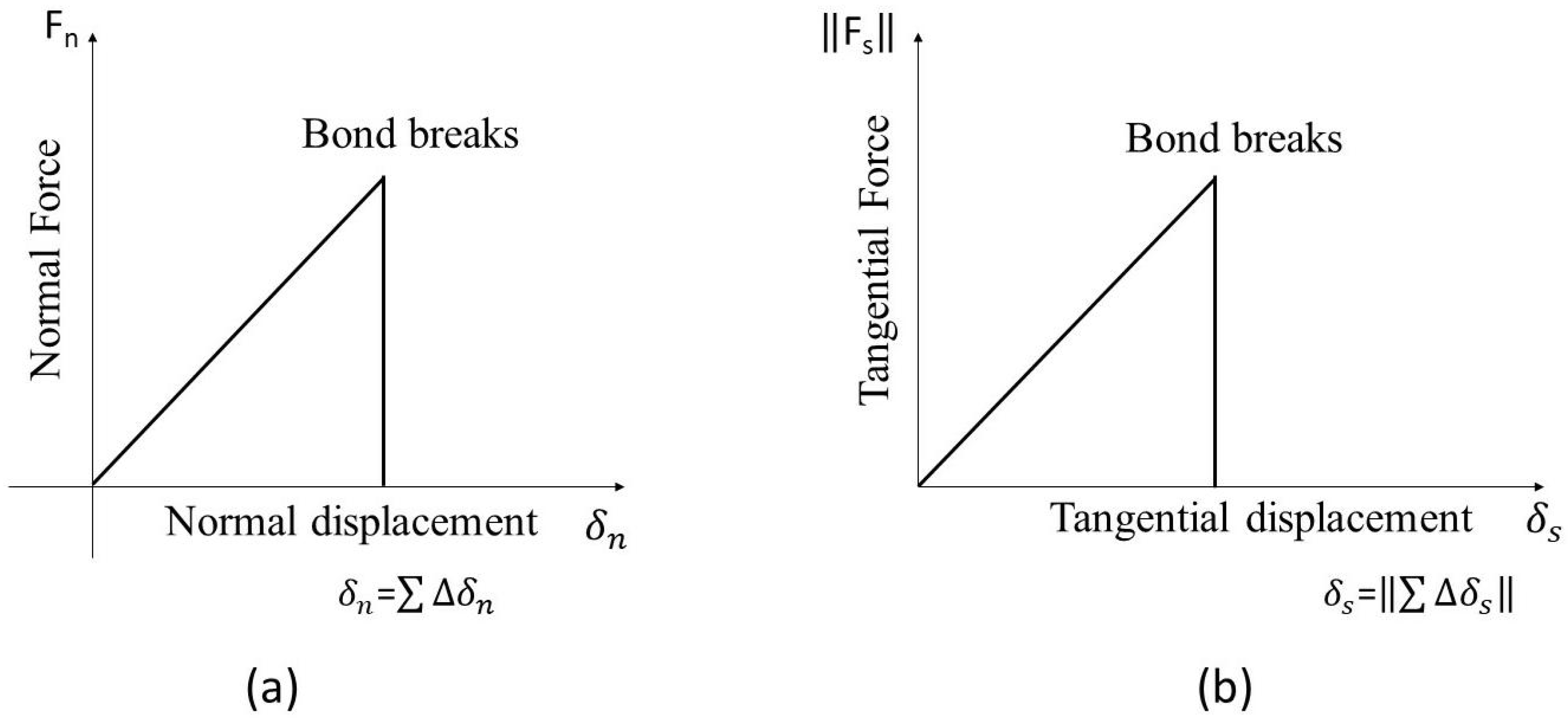
2.1. Contact Law
2.2. Thermal Transfer Theory
2.3. Simulation Procedure
2.3.1. Sample Generation
2.3.2. Sample Heating Process
2.4. Simulation of CPT
3. Results and Discussions
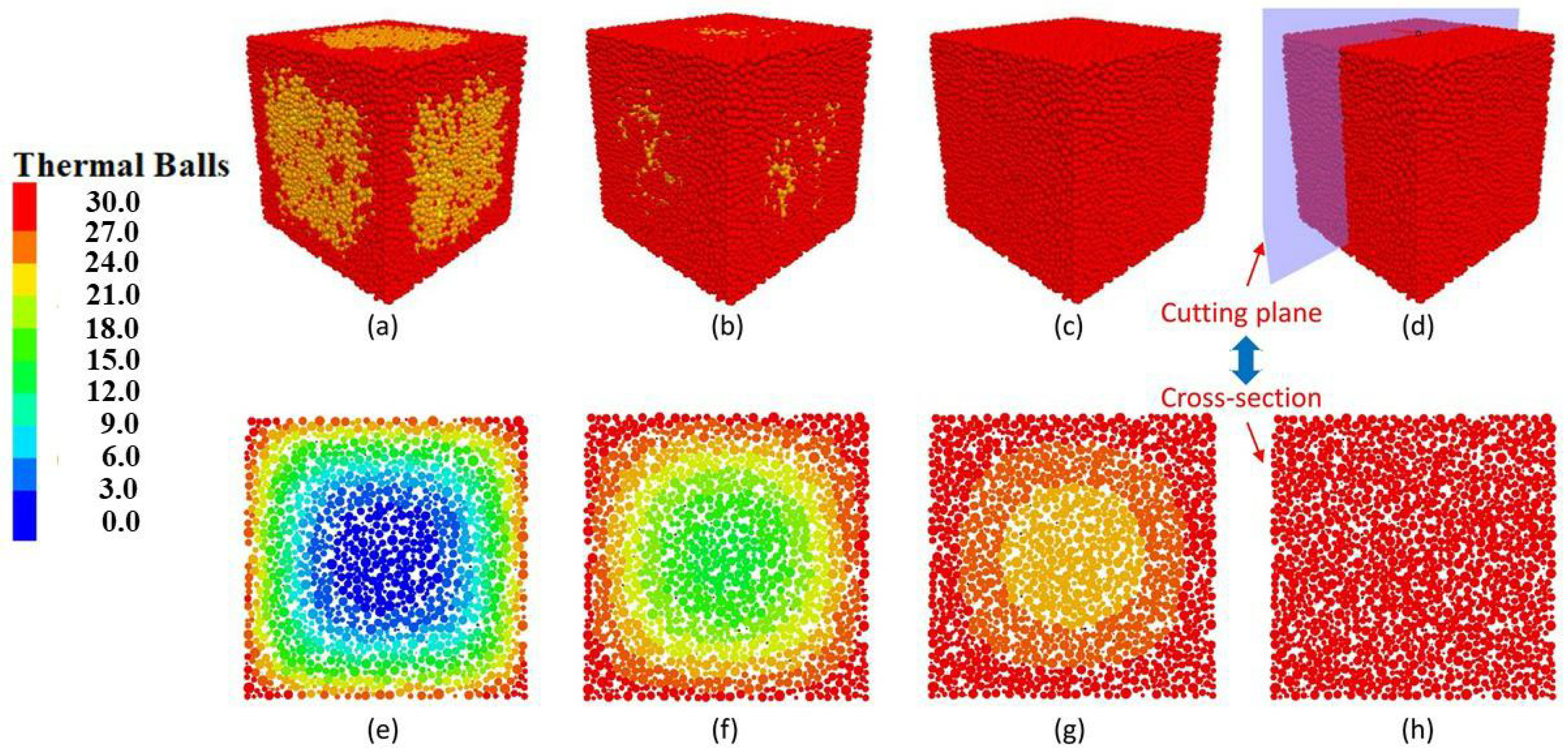
3.1. Thermal Transfer
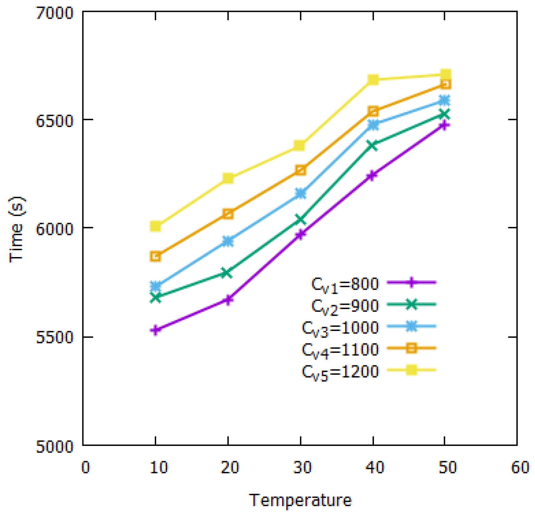
Influence of Specific Heat
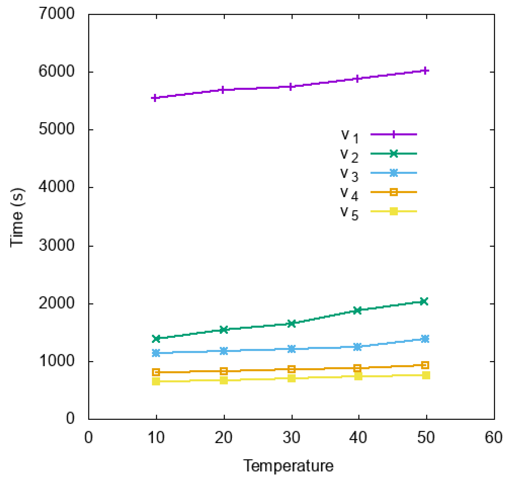
3.2. Influence of the Velocity of Thermal Conductivity
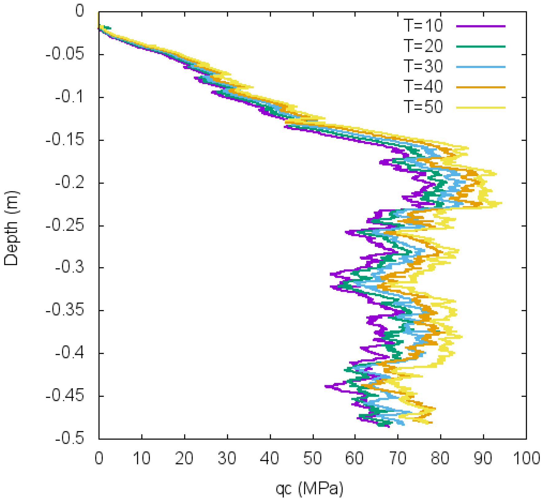
3.3. Influence of Temperatures
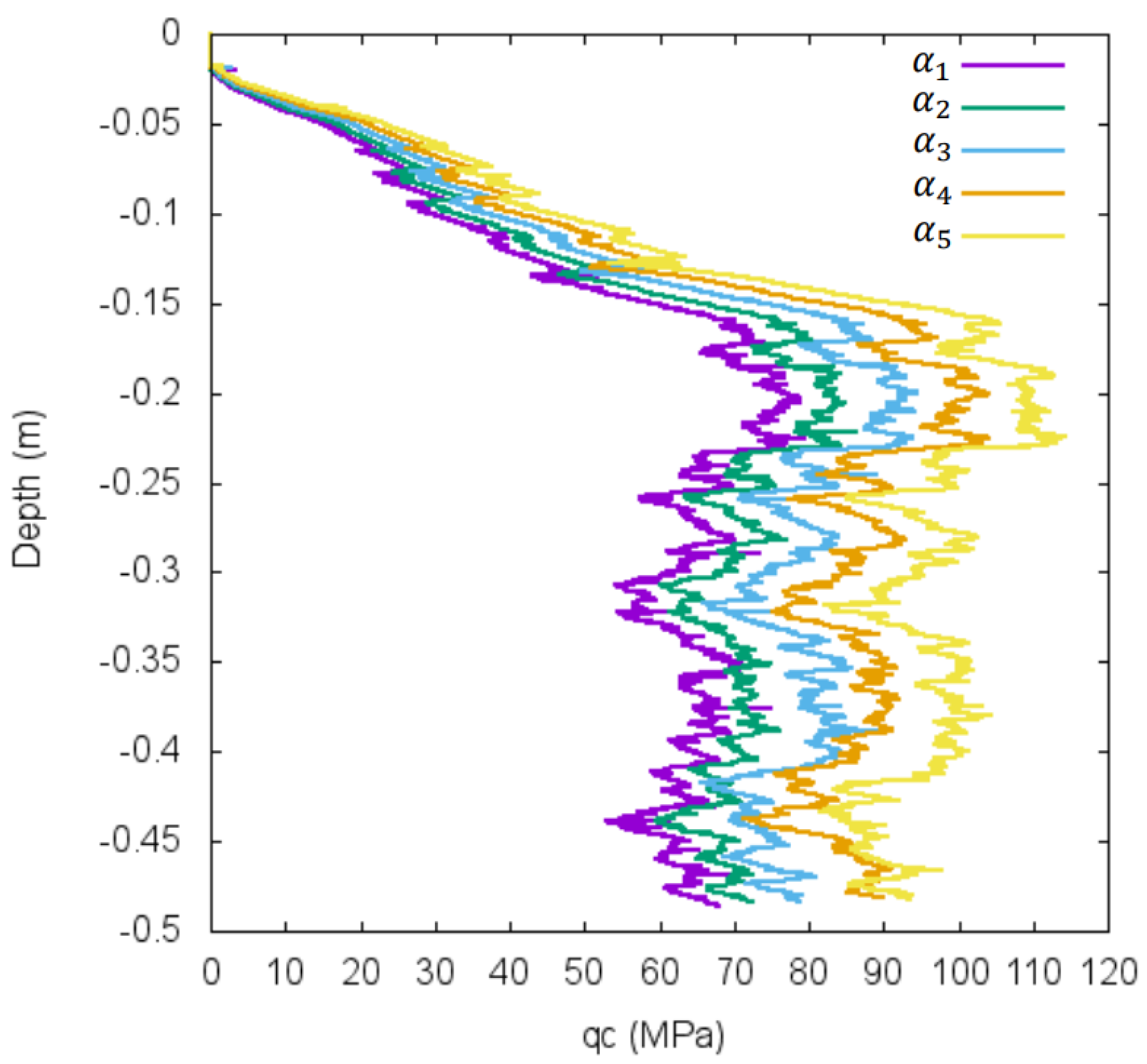
3.4. Influence of the Thermal Expansion Coefficient
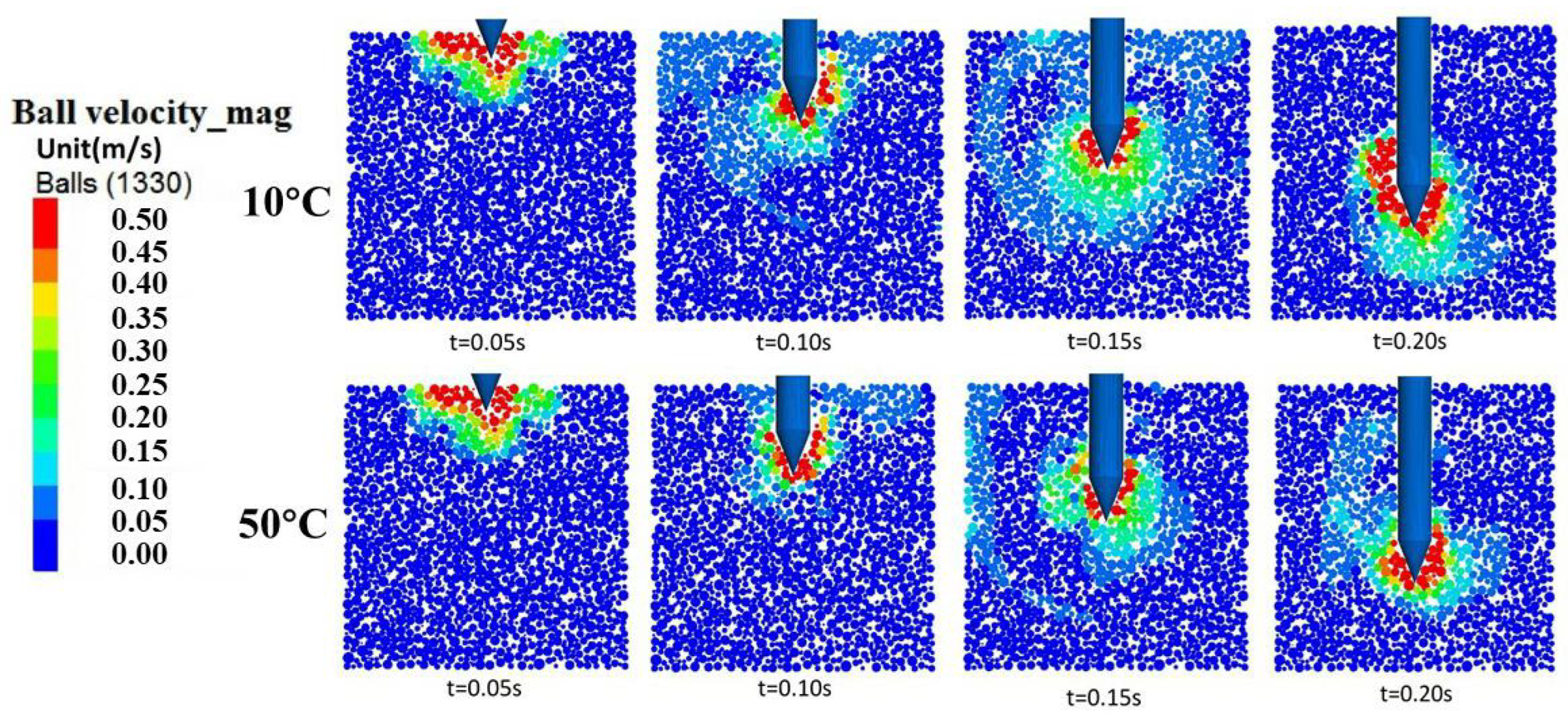
3.5. Velocity Field of the Soil Particles
4. Conclusions
- The specific heat and thermal conductivity are significantly affected by the heating time during the thermal transfer process. Generally, the total time required to heat a sample increases as specific heat increases, while it decreases as thermal conductivity increases.
- The sample becomes denser as temperature increases, based on the assumption of particle expansion during the heating process. The cone resistance of the penetrometer also increases with temperature.
- The thermal expansion coefficient of a soil particle is an important factor that affects the density of the sample. The larger the coefficient, the greater the cone resistance of the penetrometer. The velocity field and contact force chain are visualized during CPT, with maximum values occurring near the tip of the cone penetrometer.
Author Contributions
Funding
Data Availability Statement
Conflicts of Interest
Nomenclature
| Symbol | Description |
| A | area of the bond cross section |
| coefficient of restitution | |
| specific heat | |
| c | damping coefficient |
| mean diameter of the particles | |
| E | particle density |
| normal force | |
| tangential force | |
| I | inertial number |
| normal stiffness of walls | |
| normal stiffness of particles | |
| tangent stiffness of walls | |
| tangent stiffness of particles | |
| k | macroscopic conductivity |
| normal stiffness | |
| tangential stiffness | |
| length of thermal pipe | |
| m | mass of particle |
| n | porosity |
| unit normal vector | |
| cone resistance | |
| T | temperature |
| volume of particle | |
| thermal conductivity velocity | |
| w | angular velocities of particle |
| thermal expansion coefficient of particle | |
| timestep | |
| shear strain rate | |
| friction coefficient particle-boundary | |
| friction coefficient inter-particles | |
| poisson’s ratio | |
| density | |
| thermal resistance |
References
- Peric, D.; Tran, T.; Miletic, M. Effects of soil anisotropy on a soil structure interaction in a heat exchanger pile. Comput. Geotech. 2017, 86, 193–202. [Google Scholar] [CrossRef]
- Naidu, A.; Singh, D. Field Probe for Measuring Thermal Resistivity of Soils. J. Geotech. Geoenviron. Eng. 2004, 130, 213–216. [Google Scholar] [CrossRef]
- Report, H.R.B.S. (Ed.) Effects of Temperatures and Heat on Engineering Behavior of Soils; Highway Research Board: Washington, DC, USA, 1969; Volume 103. [Google Scholar]
- Cai, G.; Liu, S.; Puppala, A. Comparison of CPT charts for soil classification using PCPT data: Example from clay deposits in Jiangsu Province, China. Eng. Geol. 2011, 121, 89–96. [Google Scholar] [CrossRef]
- Cai, G.; Liu, S.; Puppala, A. Reliability assessment of CPTU-based pile capacity predictions in soft clay deposits. Eng. Geol. 2012, 141, 84–91. [Google Scholar] [CrossRef]
- Liu, S.; Shao, G.; Du, Y.; Cai, G. Depositional and geotechnical properties of marine clays in Lianyungang, China. Eng. Geol. 2011, 121, 66–74. [Google Scholar] [CrossRef]
- Cai, G.; Liu, S.; Puppala, A. Comparative performance of the international piezocone and China CPT in Jiangsu Quaternary clays of China. Transp. Geotech. 2015, 3, 1–14. [Google Scholar] [CrossRef]
- Motaghedi, H.; Armaghani, D. New method for estimation of soil shear strength parameters using results of piezocone. Measurement 2016, 77, 132–142. [Google Scholar] [CrossRef]
- Kim, R.; Lee, W.; Lee, J.S. Temperature-Compensated Cone Penetration Test Mini-Cone Using Fiber Optic Sensors. Geotech. Test. J. 2010, 33, 243–252. [Google Scholar]
- Staniec, M.; Nowak, H. The application of energy balance at the bare soil surface to predictannual soil temperature distribution. Energy Build. 2016, 127, 56–65. [Google Scholar] [CrossRef]
- Gao, H.; Shao, M. Effects of temperature changes on soil hydraulic properties. Soil Tillage Res. 2015, 153, 145–154. [Google Scholar] [CrossRef]
- Cundall, P.; Strack, O. A discrete numerical model for granular assemblies. Geotechnique 1979, 29, 47–65. [Google Scholar] [CrossRef]
- Jiang, M.; Dai, Y.; Cui, L.; Shen, Z.; Wang, X. Investigating mechanism of inclined CPT in granular ground using DEM. Granul. Matter 2014, 16, 785–796. [Google Scholar] [CrossRef] [Green Version]
- Jiang, M.; Dai, Y.; Shen, Z.; Zhang, N. Distinct Element Analyses of Inclined Cone Penetration Test in Granular Ground. Powders Grains 2013, 1542, 237–240. [Google Scholar]
- Jiang, M.; Yu, H.; Harris, D. Discrete element modelling of deep penetration in granular soils. Int. J. Numer. Anal. Methods Geomech. 2006, 30, 335–361. [Google Scholar] [CrossRef]
- Butlanska, J.; Arroyo, M.; Gens, A. 3D DEM simulations of CPT in sand. Geotech. Geophys. 2013, 1, 817–824. [Google Scholar]
- Butlanska, J.; Arroyo, M.; Gens, A. Size effects on a virtual calibration chamber. In Numerical Methods in Geotechnical Engineering; CRC Press: Boca Raton, FL, USA, 2010. [Google Scholar]
- Butlanska, J.; Arroyo, M.; Gens, A. Virtual Calibration Chamber CPT on Ticino sand. In Proceedings of the 2nd International Symposium on Cone Penetration Testing, Huntington Beach, CA, USA, 9–11 May 2010; Volume 2. [Google Scholar]
- Butlanska, J. Cone Penetration Test in a Virtual Calibration Chamber. Ph.D. Thesis, Universitat Politecnica de Catalunya, Barcelona, Spain, 2014. [Google Scholar]
- Ciantia, M.; Arroyo, M.; Butlanska, J.; Gens, A. DEM modelling of cone penetration tests in a double-porosity crushable granular material. Comput. Geotech. 2016, 73, 109–127. [Google Scholar] [CrossRef]
- McDowell, G.; Falagush, O.; Yu, H. A particle refinement method for simulating DEM of cone penetration testing in granular materials. Geotech. Lett. 2012, 2, 141–147. [Google Scholar] [CrossRef]
- Falagush, O.; McDowell, G.; Yu, H. Discrete Element Modeling of Cone Penetration Tests Incorporating Particle Shape and Crushing. Int. J. Geomech. 2015, 15, 04015003. [Google Scholar] [CrossRef]
- Falagush, O.; McDowell, G.; Yu, H.; de Bono, J. Discrete element modelling and cavity expansion analysis of cone penetration testing. Granul. Matter 2015, 17, 483–495. [Google Scholar] [CrossRef] [Green Version]
- Zhong, W.H.; Liu, H.L.; Wang, Q.; Zhang, W.G.; Li, Y.Q.; Ding, X.M.; Chen, L.L. Investigation of the penetration characteristics of snake skin-inspired pile using DEM. Acta Geotech. 2021, 16, 1849–1865. [Google Scholar] [CrossRef]
- Shi, D.D.; Yang, Y.C.; Deng, Y.B.; Xue, J.F. DEM modelling of screw pile penetration in loose granular assemblies considering the effect of drilling velocity ratio. Granul. Matter 2019, 21, 74. [Google Scholar] [CrossRef]
- Liang, Y.; Li, X. A new model for heat transfer through the contact network of randomly packed granular material. Appl. Therm. Eng. 2014, 73, 982–990. [Google Scholar] [CrossRef]
- Nguyen, V.; Cogne, C.; Guessasma, M.; Bellenger, E.; Fortin, J. Discrete modeling of granular flow with thermal transfer: Application to the discharge of silos. Appl. Therm. Eng. 2009, 29, 1846–1853. [Google Scholar] [CrossRef] [Green Version]
- Sun, L.; Wang, S.; Lu, H.; Liu, G.; Lu, H.; Liu, Y.; Zhao, F.X. Prediction of configurational and granular temperatures of particles using DEM in reciprocating grates. Powder Technol. 2015, 269, 495–504. [Google Scholar] [CrossRef]
- Sun, L.; Wang, S.; Lu, H.; Liu, G.; Lu, H.; Liu, Y.; Zhao, F. Simulations of configurational and granular temperatures of particles using DEM in roller conveyor. Powder Technol. 2014, 268, 436–445. [Google Scholar] [CrossRef]
- Itasca Consulting Group, Inc. PFC3D(Particle Flow Code in 3 Dimensions), version 5.0; user’s manual; Itasca Consulting Group, Inc.: Minneapolis, MN, USA, 2016. [Google Scholar]
- Potyondy, D.; Cundall, P. A bonded-particle model for rock. Int. J. Rock Mech. Min. Sci. 2004, 41, 1329–1364. [Google Scholar] [CrossRef]
- Holt, R.; Kjolaas, J.; Larsen, I.; Li, L.; Pillitteri, A.; Sonstebob, E. Comparison between controlled laboratory experiments and discrete particle simulations of the mechanical behaviour of rock. Int. J. Rock Mech. Min. Sci. 2005, 42, 985–995. [Google Scholar] [CrossRef]
- Jiang, M.; Sun, Y.; Li, L.; Zhu, H. Contact behavior of idealized granules bonded in two different interparticle distances: An experimental investigation. Mech. Mater. 2012, 55, 1–15. [Google Scholar] [CrossRef]
- Tomac, I.; Gutierrez, M. Formulation and implementation of coupled forced heat convection and heat conduction in DEM. Acta Geotech. 2015, 10, 421–433. [Google Scholar] [CrossRef]
- Gong, H.; Chen, Y.; Wu, S.L.; Tang, Z.Y.; Liu, C.; Wang, Z.Q.; Fu, D.B.; Zhou, Y.H.; Qi, L. Simulation of canola seedling emergence dynamics under different soil compaction levels using the discrete element method (DEM). Soil Tillage Res. 2022, 223, 105461. [Google Scholar] [CrossRef]
- Liu, L.; Li, W.L.; Lu, Y.L.; Ren, T.S.; Horton, R. Relationship between thermal and electrical conductivity curves of soils with a unimodal pore size distribution: Part 1, A unified series-parallel resistor model. Geoderma 2023, 432, 116420. [Google Scholar] [CrossRef]
- Platts, A.B.; Cameron, D.A.; Ward, J. Improving the performance of Ground Coupled HeatExchangers in unsaturated soils. Energy Build. 2015, 104, 323–335. [Google Scholar] [CrossRef]
- Guo, P.; Wang, Y.; Li, J.; Wang, Y. Thermodynamic analysis of a solar chimney power plant system with soil heat storage. Appl. Therm. Eng. 2016, 100, 1076–1084. [Google Scholar] [CrossRef]
- Janda, A.; Ooi, J. DEM modeling of cone penetration and unconfined compression in cohesive solids. Powder Technol. 2016, 293, 60–68. [Google Scholar] [CrossRef]
- Huang, W.; Sheng, D.; Sloan, S.; Yu, H. Finite element analysis of cone penetration in cohesionless soil. Comput. Geotech. 2004, 31, 517–528. [Google Scholar] [CrossRef]


| Parameter | Value | Unity |
|---|---|---|
| Number of particles, N | 45,000 | - |
| Particle radius, r | 1∼2 | cm |
| Particle density, | 2600 | kg/m |
| Local damping coefficient, c | 0.7 | - |
| Gap, | 0.1 | cm |
| Confining pressure, P | 100 | kPa |
| Friction coefficient inter-particles, | 0.3 | - |
| Friction coefficient particle-boundary, | 0.1 | - |
| Normal stiffness of particles, | 8.0 × 10 | N/m |
| Tangent stiffness of particles, | 8.0 × 10 | N/m |
| Tensile strength of bonds, | 500.0 | kPa |
| Cohesion, | 500.0 | kPa |
| Normal stiffness of walls, | 1.5 × 10 | N/m |
| Tangent stiffness of walls, | 10 | N/m |
| Timestep for mechanical study, | 1.5 × 10 | s/step |
| Thermal Parameter | Value | Unity |
|---|---|---|
| Initial temperature of soil, | 0 | C |
| Temperature of heating walls, | 10, 20, 30, 40, 50 | C |
| Specific heat, | 800 | J/(kg C) |
| Thermal conductivity, k | 1, 3, 5, 7, 9 | w/(m C) |
| Thermal expansion coefficient of particles, | 1, 2, 3, 4, 5 × 10 | - |
| Timestep for thermal transfer process, | 1 | s/step |
| Simulation | T | (cm) | Porosity n | (kPa) |
|---|---|---|---|---|
| 1 | 10 | 1.514 | 0.274 | 67.2 |
| 2 | 20 | 1.529 | 0.267 | 69.5 |
| 3 | 30 | 1.544 | 0.262 | 73.3 |
| 4 | 40 | 1.560 | 0.258 | 76.8 |
| 5 | 50 | 1.576 | 0.252 | 78.1 |
| Simulation | (cm) | Porosity n | (kPa) | |
|---|---|---|---|---|
| 1 | 1 × 10 | 1.514 | 0.274 | 66.9 |
| 2 | 2 × 10 | 1.546 | 0.261 | 72.1 |
| 3 | 3 × 10 | 1.574 | 0.252 | 79.3 |
| 4 | 4 × 10 | 1.586 | 0.243 | 88.3 |
| 5 | 5 × 10 | 1.592 | 0.233 | 92.1 |
Disclaimer/Publisher’s Note: The statements, opinions and data contained in all publications are solely those of the individual author(s) and contributor(s) and not of MDPI and/or the editor(s). MDPI and/or the editor(s) disclaim responsibility for any injury to people or property resulting from any ideas, methods, instructions or products referred to in the content. |
© 2023 by the authors. Licensee MDPI, Basel, Switzerland. This article is an open access article distributed under the terms and conditions of the Creative Commons Attribution (CC BY) license (https://creativecommons.org/licenses/by/4.0/).
Share and Cite
Huang, Y.; Sun, W.; You, H.; Wu, K. Influence of Temperature Effects on CPT in Granular Soils by Discrete Element Modeling in 3D. Geotechnics 2023, 3, 624-637. https://doi.org/10.3390/geotechnics3030034
Huang Y, Sun W, You H, Wu K. Influence of Temperature Effects on CPT in Granular Soils by Discrete Element Modeling in 3D. Geotechnics. 2023; 3(3):624-637. https://doi.org/10.3390/geotechnics3030034
Chicago/Turabian StyleHuang, Yun, Weichen Sun, Hongyi You, and Kai Wu. 2023. "Influence of Temperature Effects on CPT in Granular Soils by Discrete Element Modeling in 3D" Geotechnics 3, no. 3: 624-637. https://doi.org/10.3390/geotechnics3030034
APA StyleHuang, Y., Sun, W., You, H., & Wu, K. (2023). Influence of Temperature Effects on CPT in Granular Soils by Discrete Element Modeling in 3D. Geotechnics, 3(3), 624-637. https://doi.org/10.3390/geotechnics3030034