Accurately Predicting Quartz Sand Thermal Conductivity Using Machine Learning and Grey-Box AI Models

Abstract

The thermal conductivity of materials is a crucial property with diverse applications, particularly in engineering. Understanding soil thermal conductivity is crucial for designing efficient geothermal systems, predicting soil temperatures, and assessing soil contamination. This paper aimed to predict quartz sand thermal conductivity by using four mathematical models: multiple linear regression (MLR), artificial neural network (ANN), classification and regression random forest (CRRF), and genetic programming (GP). A grey-box AI method, GP, was used for the first time in this topic. Seven inputs affecting thermal conductivity were evaluated in the study, including sand porosity, degree of saturation, coefficient of uniformity, coefficient of curvature, mean particle size, and minimum and maximum void ratios. In predicting thermal conductivity, the MLR model performed poorly, with a coefficient of determination R² = 0.737 and a mean absolute error MAE = 0.300. Both ANN models using the Levenberg–Marquardt algorithm and the Bayesian Regularization (BR) algorithm outperformed the MLR model with an accuracy of R² = 0.916 and an error of MAE = 0.151. In addition, the CRRF model had the best accuracy of R² = 0.993 and MAE = 0.045. In addition, GP showed acceptable performance in predicting sand thermal conductivity. The R² and MAE values of GP were 0.986 and 0.063, respectively. This paper presents the best GP equation for evaluating other databases. Additionally, the porosity and saturation of the sand were found to have the greatest impact on the model results, while coefficients of curvature and uniformity had the least influence. Overall, the results of this study demonstrate that grey-box artificial intelligence models can be used to accurately predict quartz sand thermal conductivity.

1. Introduction

The thermal conductivity of soil is a significant physical characteristic that illustrates its capacity to conduct heat [1]. It affects the rate of heat transfer between the soil and the atmosphere, which in turn influences a wide range of soil processes, such as plant growth, water movement, and microbial activity [2]. The thermal conductivity of soil is influenced by factors such as composition, density, moisture content, and temperature [3]. Therefore, accurate measurement and prediction of soil thermal conductivity are crucial for many fields of science, such as agronomy, geology, environmental science, and engineering.

Soil thermal conductivity plays a significant role in geothermal heat production, particularly in geothermal reservoirs and fractured reservoirs. The thermal conductivity of the soil determines its ability to transfer heat and affects the efficiency of heat extraction from the subsurface. In geothermal reservoirs, where a high-temperature fluid is present, a higher soil thermal conductivity allows for better heat transfer and enhances the productivity of the reservoir. Similarly, in fractured reservoirs, where heat exchange occurs through permeable fractures, soil thermal conductivity influences the rate at which heat is conducted between the fractures and the surrounding soil. Understanding and optimizing soil thermal conductivity is crucial for effective geothermal heat extraction, as it directly impacts the overall performance and feasibility of geothermal energy systems [4,5,6,7,8].

Various methods have been developed for measuring soil thermal conductivity, including laboratory-based and in situ approaches. Laboratory-based methods involve heating or cooling a soil sample and measuring its temperature change over time to determine its thermal conductivity [9]. In situ methods, on the other hand, involve inserting thermal sensors into the soil and measuring the temperature gradient over a period of time [10]. While both methods can provide accurate measurements, they are time-consuming, labor-intensive, and costly. Therefore, there is a strong demand for the development of accurate and efficient predictive models for soil thermal conductivity.

Furthermore, several theoretical models were proposed by researchers. According to research by Wiener [11], porous media exhibit both upper and lower limits of thermal conductivity. The lower limit is achieved when the components are arranged in series, while the upper limit is attained when the components are arranged in parallel. Equations (1) and (2) can be used to express the effective thermal conductivities of these arrangements, respectively. These limits, known as the Wiener bounds, remain constant and do not depend on the pore structure of the medium. Equations (1) and (2) correspond to the lower and upper Wiener bounds and are expressed by λ_W^L and λ_W^U, respectively.

λ = λ_W^L = [Σϕ_α/λ_α]⁻¹ (Series),

(1)

λ = λ_W^U = Σϕ_α/λ_α (Parallel),

(2)

where ϕ_α and λ_α are the volume fraction and thermal conductivity of the α phase, respectively.

In another model, using the thermal probe method, Chen [12] conducted laboratory experiments to determine the thermal conductivities of four different types of quartz sands. Chen [12] observed that there was a linear correlation between the logarithm of the measured thermal conductivity and the porosity of the sands. Furthermore, the slope of this linear trend was affected by the degree of saturation. To model the experimental data, Chen employed an exponential function, which yielded the thermal conductivity model expressed in Equation (3). Chen [12] also proposed empirical coefficients for this model, with suggested values of 0.0022 and 0.78 for quartz sands, respectively.

λ = λ_waterⁿ · λ_solid¹⁻ⁿ [(1 − b) S_r + b]^cn,

(3)

There have been several models [13,14,15,16,17,18,19,20,21,22,23,24,25,26,27,28,29,30,31,32,33,34,35] proposed for predicting the thermal conductivity of soils. However, empirical and theoretical models can have limitations in the number of input parameters, which can decrease their accuracy and applicability.

Machine learning is a subset of artificial intelligence that involves the development of algorithms that can learn from data and make predictions or decisions based on that learning. Machine learning has been widely applied in many fields of science and engineering, including geotechnical engineering. Several studies have demonstrated the effectiveness of machine learning in predicting various properties in geotechnics, such as soil dynamics [36,37,38,39,40,41,42,43,44], slope stability, and soil cracking [45,46,47,48,49,50,51,52]. A comprehensive study has not yet been presented on the use of artificial intelligence models to predict the thermal conductivity of sand.

AI methods are used in the literature to predict the thermal conductivity of soils. Li et al. [53] compiled a large database of soil thermal conductivity data from various sources and employed six machine learning algorithms for prediction. Among these algorithms, AdaBoost performed the best, providing accurate predictions with minimal error (RMSE = 0.099). The findings highlight the potential of machine learning to accurately estimate soil thermal conductivity when sufficient data is available [53]. In another study, Kardani et al. [54] proposed hybrid computational models combining optimization algorithms and machine learning techniques to accurately predict the thermal conductivity of unsaturated soils. The best-performing model, ELM-IFF, achieved high accuracy and can be used in the initial stages of engineering projects for fast thermal conductivity determination. The proposed models show potential as alternatives to empirical models and offer improved predictive performance [54]. Furthermore, Li et al. [55] addressed the challenge of accurately predicting soil thermal conductivity by establishing a comprehensive database and utilizing an artificial neural network model. The results demonstrate strong correlations between thermal conductivity and factors such as saturation, porosity, and density. The proposed machine learning model outperforms existing models and provides a unified approach for estimating soil thermal conductivity [55].

AI algorithms have been viewed skeptically for material characterization and design due to doubts about the reliability of their complex models [56]. The lack of transparency and knowledge extraction processes in AI-based models presents a significant challenge. According to Figure 1, mathematical modeling techniques can be classified as white-box, black-box, or grey-box, depending on their level of transparency [57]. White-box models rely on first principles and offer an explanation of a system’s underlying physical relationships. Black-box models, on the other hand, do not provide any feasible structure for the model. Grey-box models identify patterns in the data and provide a mathematical structure for the model. Although artificial neural networks (ANN) are a popular black-box modeling technique used in engineering, their weight and bias representations do not provide details about the derived relationships. Genetic programming (GP), a newer grey-box modeling technique, uses an evolutionary process to develop explicit prediction functions, which makes it more transparent than other machine learning methods, especially black-box methods such as ANN and classification and regression random forest (CRRF). GP’s mathematical structures can be leveraged to gain crucial insights into the system’s performance. GP models have shown promising results in terms of accuracy and efficiency.

This study utilized four different mathematical models, including a multiple linear regression (MLR) model as a statistical model, two black-box artificial intelligence models—the classic artificial neural network (ANN), which is the most commonly used AI model in geotechnical engineering, and the classification and regression random forest (CRRF), a more recent model. Additionally, a grey-box AI method, the genetic programming (GP) method, was employed for the first time for predicting thermal conductivity. Subsequently, the importance of input parameters was assessed, and a sensitivity analysis was conducted. While the cost of measuring thermal conductivity in a laboratory setting is typically not high compared to other parameters in the equation, the focus of this study was to demonstrate an alternative approach. The objective was to explore the possibility of calculating thermal conductivity using common geotechnical parameters, without the need for a separate thermal conductivity test. By leveraging readily available data and utilizing established geotechnical parameters, this research aimed to provide a cost-effective method for estimating thermal conductivity.

2. Database Collection and Processing

This study uses an 80-laboratory database originally studied by Chen [12] that examined the impact of porosity and degree of saturation on the thermal conductivity of sands. Chen [12] conducted a series of tests utilizing a laboratory thermal probe to gather the data. The collected database is represented as three-dimensional diagrams in Figure 2.

The present database comprises seven inputs, featuring measurements of degree of saturation, porosity, maximum and minimum porosity, mean or average particle size (D₅₀), coefficient of curvature (C_c), and uniformity coefficient (C_u), with soil thermal conductivity as the output variable. Notably, this database represents one of the largest databases of laboratory-derived soil thermal conductivity measurements in the literature, characterized by a substantial number of entries.

As depicted in Figure 3, the influence of soil saturation and porosity on the coefficient of soil thermal conductivity is demonstrated. The findings indicate that an increase in the degree of soil saturation is associated with an elevation in the coefficient of thermal conductivity. It may be due to the fact that water has a higher thermal conductivity than air, and therefore, the presence of water in the soil can enhance thermal conductivity of the soil. As the degree of soil saturation increases, the proportion of water in the soil also increases, resulting in an increase in soil thermal conductivity. On the other hand, the decrease in soil thermal conductivity with increasing soil porosity could be attributed to the fact that air has a lower thermal conductivity than solid materials such as soil particles. Therefore, the presence of air in the soil can decrease its thermal conductivity. As soil porosity increases, the proportion of voids in the soil also increases, leading to a decrease in soil thermal conductivity.

To effectively demonstrate the impact of porosity on thermal conductivity, Figure 4 presents the variation of porosity across different degrees of saturation for a sand sample in a study by Chen [12]. According to Figure 4, under similar conditions, an increase in the porosity results in a decrease in the sand’s thermal conductivity.

Table 1. Descriptive statistics for the collected database.

Variable		Observations	Minimum	Maximum	Mean	Std. Deviation
Output	λ (Wm−1K−1)	80	0.150	2.580	1.257	0.679
Inputs	Sr (%)	80	0.000	100.000	37.000	35.947
	n	80	0.354	0.547	0.459	0.053
	Max-n	80	0.472	0.547	0.514	0.034
	Min-n	80	0.354	0.434	0.405	0.033
	D50 (mm)	80	0.130	0.580	0.340	0.161
	Cc	80	0.040	1.736	0.699	0.706
	Cu	80	0.267	3.600	1.632	1.361

presents the statistical characteristics of the database used in this study, including minimum, maximum, and mean values for both inputs and outputs. These descriptive statistics provide useful insights into the distribution and characteristics of the data, which can inform model selection and optimization efforts in subsequent analyses.

It is worth mentioning that for the computation of C_c and C_u values, the particle size distribution graphs presented in Chen’s [12] study were utilized to extract the corresponding D₁₀, D₃₀, D₅₀, and D₆₀ values. Subsequently, Equations (4) and (5) were employed to calculate the C_c and C_u values.

C_u = D₆₀/D₁₀

(4)

$${\mathrm{C}}_{\mathrm{c}}={{\mathrm{D}}_{30}}^2/({\mathrm{D}}_{60} \times {\mathrm{D}}_{10})$$

(5)

2.1. Outliers

In a random sample, an outlier is defined as an observation that significantly deviates from the other values, leaving the determination of abnormality to the analyst’s discretion. Detecting abnormal observations is a crucial step in statistical analysis and is accomplished by first characterizing normal observations. The overall shape of the graphed data is examined, and unusual observations that are considerably far from the bulk of the data, referred to as outliers, are identified. Two graphical techniques used to identify outliers are scatter plots and box plots, with the latter using the median, lower quartile, and upper quartile to display the behavior of data in the middle and at the ends of distributions. Additionally, box plots employ fences to identify extreme values in the distribution tails, where points beyond an inner fence are mild outliers and those beyond an outer fence are extreme outliers.

In this study, a dataset consisting of 80 observations was considered, and a box plot was employed to identify outliers. The process involves computing the median, lower quartile, upper quartile, and interquartile range, and then calculating the lower and upper fences. Based on the computed fences and the data in Figure 5, no point that exceeds the extreme values is identified.

2.2. Testing and Training Databases

The database used in the study was partitioned into two distinct categories, namely training and testing databases. To accomplish this, a random selection process was employed to allocate 80% of the data to the training database and the remaining 20% to the testing database.

Table 2. Descriptive statistics for the training database.

Variable		Observations	Minimum	Maximum	Mean	Std. Deviation
Output	λ (Wm−1K−1)	64	0.150	2.580	1.319	0.667
Inputs	Sr (%)	64	0.000	100.000	39.766	36.323
	n	64	0.354	0.547	0.458	0.053
	Max-n	64	0.472	0.547	0.513	0.033
	Min-n	64	0.354	0.434	0.405	0.032
	D50 (mm)	64	0.130	0.580	0.350	0.159
	Cc	64	0.040	1.736	0.765	0.715
	Cu	64	0.267	3.600	1.762	1.375

and

Table 3. Descriptive statistics for the testing database.

Variable		Observations	Minimum	Maximum	Mean	Std. Deviation
Output	λ (Wm−1K−1)	16	0.150	2.200	1.009	0.695
Inputs	Sr (%)	16	0.000	100.000	25.938	33.177
	n	16	0.354	0.547	0.465	0.054
	Max-n	16	0.472	0.547	0.516	0.036
	Min-n	16	0.354	0.434	0.404	0.037
	D50 (mm)	16	0.130	0.580	0.299	0.166
	Cc	16	0.040	1.736	0.434	0.619
	Cu	16	0.267	3.600	1.110	1.209

present a comprehensive overview of the statistical characteristics of various parameters, such as minimum, maximum, and average values for the training and test databases, respectively.

The results of the statistical analysis indicate that the characteristics of the two databases are similar, which suggests that the data used for training the artificial intelligence model is representative of the data used for testing the model. This similarity in statistical properties between the training and test databases is likely to enhance the accuracy and robustness of the model developed. The findings from this study imply that the use of representative and well-characterized data is crucial for developing effective and reliable artificial intelligence models.

2.3. Linear Normalizations

In the context of a database, individual input or output variables are associated with specific units of measurement. One commonly employed approach to mitigate the influence of units and enhance the efficiency of artificial intelligence training involves normalizing the data by rescaling it to fall within a common range (e.g., between zero and one). This normalization process is accomplished by applying a linear transformation function, which is described below.

$$X_{norm}=\frac{X-X_{min}}{X_{max}-X_{min}}$$

(6)

The four terms in this equation are X_max, X_min, X, and X_norm, which correspond to maximum, minimum, actual, and normalized values, respectively.

3. Data-Driven Modeling

Initially, MLR models were employed to find the best model that balanced accuracy and user friendliness. Later, more advanced artificial intelligence models like ANN, CRRF, and GP were utilized. MLR also offers Pearson correlations (r) to assess the level of linearity between variables. All AI methods followed a progression from simpler models to more complex ones to improve accuracy.

3.1. Multiple Linear Regression (MLR)

MLR, or multiple linear regression, is a statistical approach used to predict an output variable based on multiple independent input variables [60]. MLR is an enhanced version of linear regression, which involves a single input variable and one output variable.

In MLR, the relationships between input and output parameters (Equation (7)) are assumed to be linear [61]. Additionally, data normalization is implemented in this method.

$$y={\beta }_0+{\beta }_1{X}_1+\dots +{\beta }_n{X}_n+\epsilon ,$$

(7)

In this equation, y is the predicted value, β₀ is the y-intercept when all other parameters are 0, X₁ and X_n are the first and last independent variables, β₁, β_n are the regression coefficients of the first and last independent variables, and $\epsilon$ is the model error.

In MLR, the optimal line is determined by selecting regression coefficients that minimize the model’s error. MLR was used before ANN, CRRF, and GP models to assess the accuracy of linear regression, which is considered one of the simplest regression methods.

3.2. Artificial Neural Network (ANN)

Artificial Neural Network (ANN) is a powerful method used to model complex relationships that lack established mathematical equations. It consists of artificial neurons and is commonly employed to fit nonlinear statistical data. In ANN, the relationships between input and output parameters are determined based on the connection strength between neurons, referred to as “weight”. The network aims to optimize the weight matrix through iterative practice and adjustment, using techniques such as the back-propagation paradigm. In this study, two back-propagation algorithms, namely the Levenberg–Marquardt (LM) algorithm [62] and the Bayesian Regularization (BR) algorithm [63], were employed.

The ANN architecture comprises three main components: the input layer, hidden layer(s), and output layer. For each algorithm (LM and BR), different configurations were considered, ranging from one to five hidden layers. The transfer functions used within each neuron were log-sig and tan-sig. In this study, five different ANN architectures were modeled for each algorithm, varying the number of hidden layers. Additionally, through trial and error, each hidden layer consisted of 60 neurons, and each network was trained five times.

3.3. Classification and Regression Random Forests (CRRF)

In 2001, Breiman introduced random forest (RF) as a method based on decision trees. RF combines decision trees with bootstrap aggregation (e.g., Shapire et al. [64]) or bagging [65] to reduce errors in classification and regression tasks. Boosting, on the other hand, assigns extra weight to earlier predictions that were incorrectly predicted by applying successive trees. This results in a weighted vote for the final prediction.

Bagging involves constructing trees independently using bootstrap samples of the dataset, without relying on earlier trees for construction. The outcome is predicted through a simple majority vote. Breiman extended this concept in 2001 by introducing random forests, which introduce an additional level of randomness to bagging. Random forests construct classification or regression trees using different bootstrap samples from the data and change how the trees are constructed.

In standard trees, each node is split based on the best split among all variables. In random forests, each node is split based on a randomly selected subset of predictors at that node. Surprisingly, this approach proves to be highly effective compared to other classifiers like discriminant analysis, support vector machines, and neural networks. It is also resilient to overfitting [66]. The method is user-friendly with only two parameters: the number of random variables in a node and the number of trees in the forest. It is typically not sensitive to their values.

Considering a single tree within the forest, let us examine Ti ∈ ℝMi × Ni, where i represents the ith partition of the samples (Mi) and features (Ni). Ti is randomly selected by sampling with replacement from the original data (X ∈ ℝM × N) using a bootstrap method [67].

To split the available samples (Mi) at each node, a feature from the subset Ni is considered. The Gini Index [68] is employed to identify the optimal feature and cutoff value for splitting. Samples with values greater than the cutoff are directed to the right node (vR), while samples below the cutoff move to the left node (vL). This splitting process is repeated multiple times, leading the samples from the root node (vn) to terminal nodes, also known as terminal leaves. The terminal leaves provide predictions based on the samples contained within them.

The ensemble predictions of the random forest (Z ∈ ℝMi × Ni) are obtained by combining the results of the individual trees. For classification, the majority vote rule is typically used, while for regression problems, the results are averaged [69].

$$\mathrm{Classification}: {\mathrm{Z}}_i = {\mathrm{mode}}_{n=1\dots N_{trees}} {\mathrm{Z}}_n,$$

(8)

$$\mathrm{Regression}: {\mathrm{Z}}_i=\frac{1}{N_{trees}}{{\displaystyle \sum }}_{n=1}^{N_{trees}}{Z}_n,$$

(9)

where $N_{trees}$ is the total number of trees used in the RF.

3.4. Genetic Programming (GP)

Genetic programming (GP) is a subfield of artificial intelligence and machine learning that uses evolutionary algorithms to generate computer programs. It was first proposed by John Koza in the early 1990s [70] and has since become a popular research area with many applications in various fields. GP has since been applied to a wide range of problems, including image recognition, classification, and prediction. Advantages of genetic programming include the following:

-

Flexibility: GP can be used to solve a wide range of problems in various fields, including engineering, finance, and biology.

-

Automatic programming: GP can generate computer programs automatically without human intervention, which can save time and effort.

-

Optimization: GP can optimize complex functions that are difficult to solve using traditional methods.

-

Creativity: GP can generate solutions that are unexpected and creative, which can lead to new discoveries.

Disadvantages of genetic programming include:

-

Time-consuming: GP can be computationally expensive, especially for large search spaces.

-

Lack of transparency: The generated programs can be difficult to understand and interpret, which can make it hard to validate the results.

-

Limited performance: GP can be sensitive to the choice of parameters, and it may not always find the optimal solution.

-

Overfitting: GP can generate programs that are overfitted to the training data, which may not generalize well to new data.

4. Results

Evaluating different models is crucial in the development of Artificial Intelligence (AI) systems. Statistical parameters play a key role in facilitating this assessment process. Equations (10)–(15) define these parameters, which are essential for evaluating the performance of AI models. They include Mean Absolute Error (MAE), Mean Squared Error (MSE), Root Mean Squared Error (RMSE), Mean Squared Logarithmic Error (MSLE), Root Mean Squared Logarithmic Error (RMSLE), and Coefficient of Determination (R²). By utilizing these parameters, researchers and developers can effectively measure and compare the performance of different AI models.

$$\mathrm{MAE}=\frac{{{\displaystyle \sum }}_N\left(X_{\mathrm{m}}-X_{\mathrm{p}}\right)}{N},$$

(10)

$$\mathrm{MSE}=\frac{{{\displaystyle \sum }}_N{\left(X_{\mathrm{m}}-X_{\mathrm{p}}\right)}^2}{N},$$

(11)

$$\mathrm{RMSE}=\sqrt{\frac{{{\displaystyle \sum }}_N{\left(X_{\mathrm{m}}-X_{\mathrm{p}}\right)}^2}{N}}$$

(12)

$$\mathrm{MSLE}=\frac{{{\displaystyle \sum }}_N{\left({\log }_{10}\left[X_{\mathrm{m}}+1\right]-{\log }_{10}\left[X_{\mathrm{p}}+1\right]\right)}^2}{N}$$

(13)

$$\mathrm{RMSLE}=\sqrt{\frac{{{\displaystyle \sum }}_N{\left({\log }_{10}\left[X_{\mathrm{m}}+1\right]-{\log }_{10}\left[X_{\mathrm{p}}+1\right]\right)}^2}{N}}$$

(14)

$$R^2={\left[\frac{{{\displaystyle \sum }}_N\left(X_{\mathrm{m}}-\overline{X_{\mathrm{m}}}\right)\left(X_{\mathrm{p}}-\overline{X_{\mathrm{p}}}\right)}{{{\displaystyle \sum }}_N{\left(X_{\mathrm{m}}-\overline{X_{\mathrm{m}}}\right)}^2{{\displaystyle \sum }}_N{\left(X_{\mathrm{p}}-\overline{X_{\mathrm{p}}}\right)}^2}\right]}^2$$

(15)

where N = number of datasets; X_m and X_p = actual and predicted values, respectively; and $\overline{{\mathrm{X}}_{\mathrm{m}}}$ and $\overline{{\mathrm{X}}_{\mathrm{p}}}$= average of the actual and predicted values, respectively. Ideally, the model should have R² = 1 and MAE, MSE, RMSE, MSLE, and RMSLE values of 0.

4.1. Multiple Linear Regression (MLR)

Prior to investigating the linear model, it is essential to assess the linear correlation between the variables.

Table 4. Pearson matrix for input and output parameters.

	Sr	n	Max-n	Min-n	D50	Cc	Cu	λ
Sr	1	0.072	0.058	0.061	−0.077	−0.029	−0.037	0.781
n	0.072	1	0.601	0.600	0.108	0.006	−0.019	−0.102
Max-n	0.058	0.601	1	0.758	0.164	−0.120	−0.158	0.150
Min-n	0.061	0.600	0.758	1	0.154	0.140	0.094	0.146
D50	−0.077	0.108	0.164	0.154	1	0.395	0.442	−0.079
Cc	−0.029	0.006	−0.120	0.140	0.395	1	0.797	−0.055
Cu	−0.037	−0.019	−0.158	0.094	0.442	0.797	1	−0.066
λ	0.781	−0.102	0.150	0.146	−0.079	−0.055	−0.066	1

presents the Pearson correlation matrix between the input and output parameters. The findings indicate that the soil saturation degree parameter exhibits the highest Pearson coefficient value of 0.781 among the input parameters and the output parameter. Additionally, the C_u and C_c parameters show the strongest linear correlation among the input parameters, with a Pearson correlation of 0.797. These observations suggest a lack of substantial linear association between the input parameters and the output parameters.

The present investigation employed a multiple linear regression (MLR) model to examine the relationship between a dependent variable and several independent variables. The selection of the independent variables was based on their theoretical relevance and statistical significance. Prior to analysis, the model was tested for multicollinearity, and assumptions of normality, linearity, and homoscedasticity were evaluated. The performance of the best MLR in predicting thermal conductivity is illustrated in Figure 6, which displays the predicted values against the actual values. The results of the analysis reveal that the MLR model is not particularly effective in accurately predicting thermal conductivity values, as evidenced by the deviation between the predicted and actual values. These findings underscore the need for more sophisticated modeling approaches that can better capture the complex relationships between the input and output variables.

Table 5. Overall performance of the best MLR model to predict the soil thermal conductivity for both training and testing datasets.

Metric	Training Dataset	Testing Dataset
MAE	0.205	0.300
MSE	0.059	0.119
RMSE	0.242	0.345
MSLE	0.018	0.044
RMSLE	0.134	0.210
R²	0.866	0.737

presents the accuracy metrics of the best MLR model, which were computed to evaluate the model’s performance and validate its accuracy. These metrics provide important insights into the MLR model’s ability to capture the underlying patterns and relationships between the input and output variables. The results in Table 5 suggest that the MLR model did not perform well in predicting soil thermal conductivity, with higher values for MAE, MSE, and RMSE indicating low accuracy for both the training and testing datasets. The MSLE and RMSLE values were also relatively high, indicating that the model was not accurate in predicting the logarithm of the output variable. The R² value was relatively high for the training dataset (0.866), indicating an almost perfect fit between the input and output variables. However, the R² value for the testing database was lower (0.737), indicating that the MLR model’s performance was less accurate for new, unseen data.

The optimal linear equation derived from the MLR model is presented below.

λ = −0.3459 + 0.0162 × S_r − 4.4898 n + 4.7330 × n_max + 1.6763 × n_min − 9.9246 × 10⁻² × D₅₀,

(16)

The equation incorporates five input variables, namely degree of saturation (S_r), porosity (n), maximum and minimum porosity, and average size of particles. This observation implies that the remaining input variables are relatively less significant in predicting the soil thermal conductivity within the MLR model.

4.2. Artificial Neural Network (ANN)

Following the unsuccessful performance of the MLR model, the artificial neural network (ANN) method, which is a classic and widely used approach in artificial intelligence, was employed. In this regard, two distinct algorithms, namely BR and LM, with varying numbers of neurons ranging from 0 to 60, were examined. The performance of the optimal ANN model is illustrated in Figure 7, which displays the predicted values versus the actual values obtained from the experiment. The findings suggest that the ANN method outperformed the MLR method and exhibited satisfactory predictive capabilities in determining soil thermal conductivity test values. Specifically, the optimal ANN model, which comprises 14 neurons, was developed using the BR algorithm.

Table 6. Overall performance of the best ANN model to predict the soil thermal conductivity for both training and testing datasets.

Metric	Training Dataset	Testing Dataset
MAE	0.158	0.151
MSE	0.036	0.038
RMSE	0.189	0.195
MSLE	0.007	0.007
RMSLE	0.086	0.081
R²	0.918	0.916

presents the overall performance of the best Artificial Neural Network (ANN) model in predicting the soil thermal conductivity for both training and testing datasets. Various performance metrics were employed to evaluate the accuracy of the model. Mean Absolute Error (MAE) represents the average absolute difference between the predicted and actual values, expressed as a percentage. The values for the training dataset and testing dataset are 0.158 and 0.151, respectively. Furthermore, Mean Squared Error (MSE) represents the average squared difference between the predicted and actual values, expressed as a percentage. The values for the training dataset and testing dataset are 0.036 and 0.038, respectively. Root Mean Squared Error (RMSE) represents the square root of the average squared difference between the predicted and actual values, expressed as a percentage. The values for the training dataset and testing dataset are 0.189 and 0.195, respectively. Mean Squared Log Error (MSLE) represents the average of the squared logarithmic difference between the predicted and actual values, expressed as a percentage. The values for the training dataset and testing dataset are 0.007 and 0.007, respectively. Root Mean Squared Log Error (RMSLE) represents the square root of the average of the squared logarithmic difference between the predicted and actual values, expressed as a percentage. The values for the training dataset and testing dataset are 0.086 and 0.081, respectively. R-squared (R²) represents the coefficient of determination, which measures the proportion of variance in the dependent variable that can be explained by the independent variables. The values for the training dataset and testing dataset are 0.918 and 0.916, respectively. These results demonstrate the strong predictive capabilities of the best ANN model in determining soil thermal conductivity, as evidenced by the low values of MAE, MSE, RMSE, MSLE, and RMSLE and the high value of R² for both the training and testing datasets.

One crucial point in ANN models pertains to determining the appropriate number of hidden layers and neurons in each layer. The analysis conducted in this study reveals that, within the range of 1 to 6 hidden layers, the optimal number of hidden layers is 3. Based on the model analysis, the ANN model’s accuracy (R²) attains its peak, and the error (MAE) rate reaches its lowest level after 19 neurons, signifying that this is the most optimal number of neurons for the given database.

4.3. Classification and Regression Random Forest (CRRF)

To obtain the most optimal CRRF model, several CRRF models were tested, and various influential parameters, such as Trees and Forest parameters, were modified.

Table 7. The specifications of the best CRRF.

Trees Parameters					Forest Parameters
Min. node size	Min. son size	Max depth	Mtry	CP	Sampling	Sample size	Number of trees
3	2	13	2	0.00001	Random with replacement	55	300

shows the specifications of the best CRRF model. The CRRF model consists of a forest of decision trees, and the table provides information on the specific parameters used to create this forest. The table is divided into two parts: the Trees parameters and the Forest parameters. The Trees parameters describe the characteristics of the individual decision trees in the forest, while the Forest parameters describe how the forest was constructed. The Trees parameters specify the minimum node size, the minimum son size, and the maximum depth of each decision tree. The minimum node size refers to the minimum number of observations required in a node for it to be split further. The minimum son size is the minimum number of observations required in a terminal node, which is a node that does not split further. The maximum depth of a tree is the maximum number of levels that the tree can have.

The Forest parameters specify the number of variables considered for each split, the complexity parameter (CP), the sampling method, the sample size, and the number of trees in the forest. The M_try parameter specifies the number of variables to be randomly sampled at each node for splitting. The CP parameter controls the complexity of the model, with smaller values leading to more complex models. The sampling method determines how the samples are drawn from the dataset. In this case, it is random with replacement, meaning that each observation has an equal chance of being selected for each sample. The sample size is the number of observations in each sample, and the number of trees is the total number of decision trees in the forest.

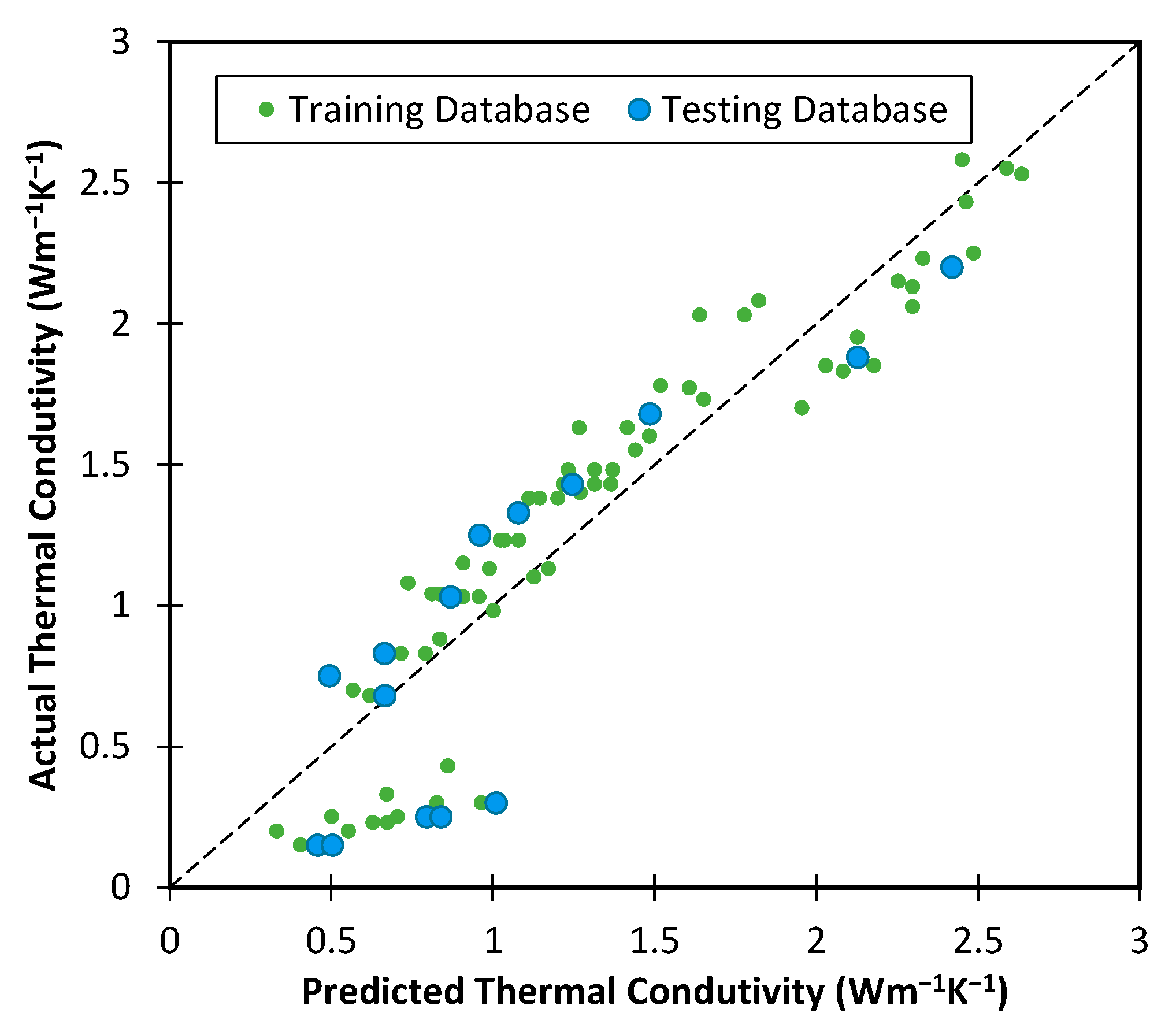
The predicted values obtained from the CRRF model versus the actual laboratory values are plotted in Figure 8. The evaluation of the results indicates that the CRRF model has achieved significantly better performance compared to both the MLR model and the ANN model.

Table 8. Overall performance of the best CRRF model to predict the soil thermal conductivity for both training and testing datasets.

Metric	Training Dataset	Testing Dataset
MAE	0.081	0.045
MSE	0.010	0.003
RMSE	0.101	0.056
MSLE	0.003	0.001
RMSLE	0.050	0.038
R²	0.976	0.993

summarizes the performance of the best CRRF model in predicting soil thermal conductivity for both the training and testing datasets. The results indicate that the CRRF model performed well in both datasets, with low values for metrics such as MAE, MSE, RMSE, MSLE, and RMSLE, indicating good accuracy in predicting soil thermal conductivity. The high value of R² for both datasets (0.976 for the training dataset and 0.993 for the testing dataset) suggests that a significant proportion of the variance in soil thermal conductivity can be explained by the predictors used in the model.

4.4. Genetic Programming (GP)

Another model investigated in this study is a grey-box model called genetic programming (GP). To achieve the best possible performance, various iterations of this model were tested, and the most optimal configuration was determined.

Table 9. The properties of the optimum GP model.

Population		Probability of GP Operations			Selection			Tree Structure Level		Random Constants		GP imp. Parameters
Size	Initialization	Crossover	Mutation	Reproduction	Elitism	Method	Tour Size	Max. initial	Max. operation	From-to	Count	Brood size
100	HalfHalf	0.99	0.99	0.2	1	Rank Selection	1.6	6	6	0–1	3	7

provides a summary of the critical parameters employed in the GP model. These properties include several parameters that were adjusted to achieve the best possible performance of the model in predicting the target variable.

Table 9 lists various parameters such as population size, probability of GP operations, selection method, tree structure level, random constants, and GP implementation parameters. The population size was set at 100, and the probability of GP operations was set at 0.99 for both crossover and mutation operations. The selection method used was Rank Selection, and the tour size was set at 1.6. The maximum initial tree depth and maximum tree depth for all GP operations were set at 6. Moreover, the GP model was initialized using the HalfHalf method, and the tree structure level was set to range from 0 to 1 with a count of 3. Finally, the GP implementation parameters included a brood size of 7 and a reproduction probability of 0.2. These parameters were tuned to optimize the GP model’s performance in predicting the target variable.

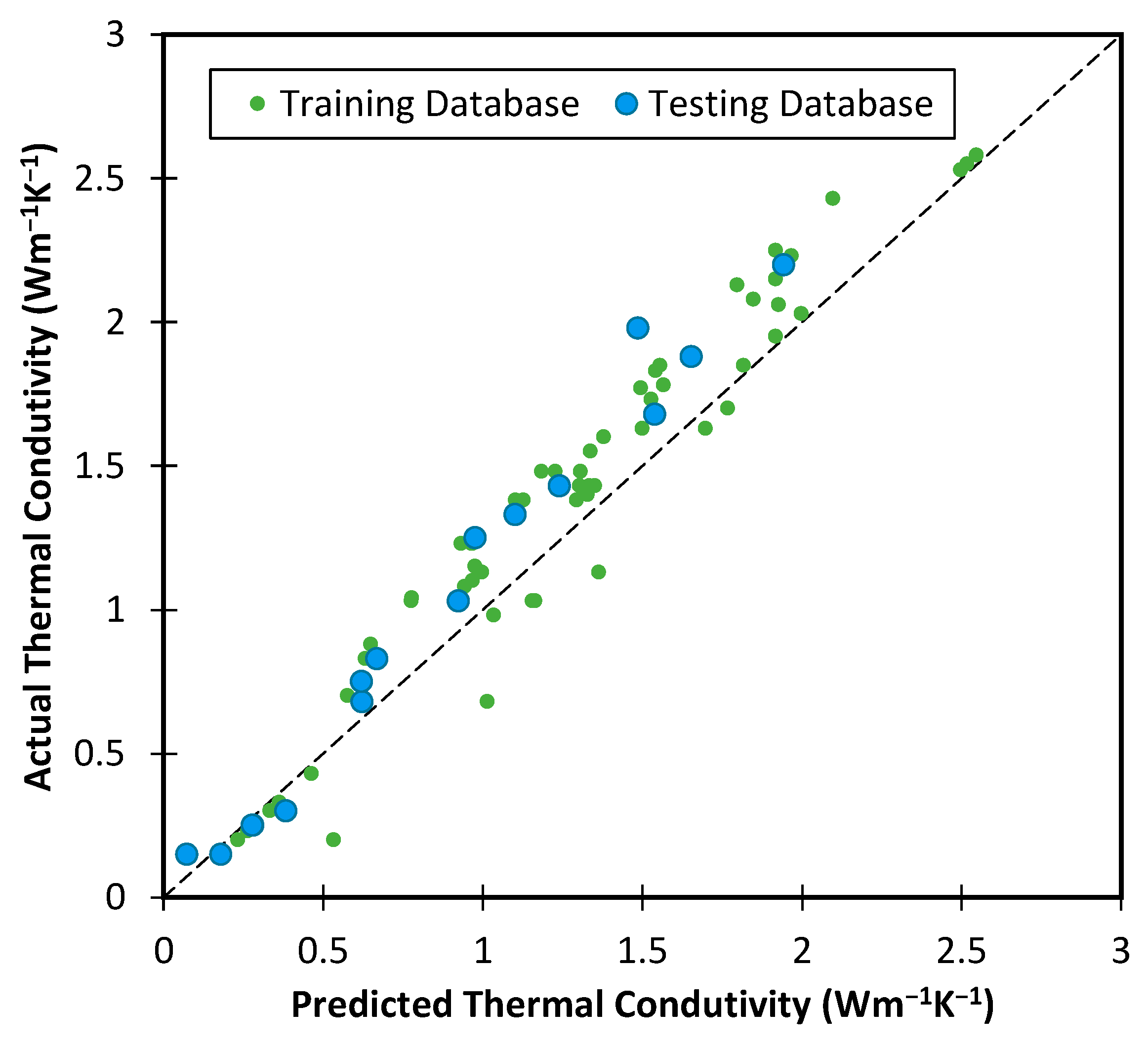
Based on the results obtained from the testing and training databases, Figure 9 illustrates the comparison of predicted thermal conductivity values by the GP model with the actual values. The performance of the GP model in predicting soil thermal conductivity is very satisfactory.

Table 10. Overall performance of the best GP model to predict the soil thermal conductivity for both training and testing datasets.

Metric	Training Dataset	Testing Dataset
MAE	0.075	0.063
MSE	0.008	0.006
RMSE	0.088	0.080
MSLE	0.002	0.001
RMSLE	0.039	0.038
R²	0.982	0.986

illustrates the comprehensive evaluation of the top-performing genetic programming (GP) model for predicting soil thermal conductivity in both the training and testing datasets. Various metrics were utilized to assess the performance of the GP model.

For the training dataset, the GP model achieved an MAE of 0.075, an MSE of 0.008, and an RMSE of 0.088, indicating that the model had a relatively small average error in predicting soil thermal conductivity for the training dataset. The MSLE and RMSLE values were 0.002 and 0.039, respectively, indicating that the model had a good fit to the data. The R² value of 0.982 indicates that the model explained a significant portion of the variance in the data.

Similarly, for the testing dataset, the GP model achieved an MAE of 0.063, an MSE of 0.006, and an RMSE of 0.080, indicating that the model had a relatively small average error in predicting soil thermal conductivity for the testing dataset. The MSLE and RMSLE values were 0.001 and 0.038, respectively, indicating that the model had a good fit to the data. The R² value of 0.986 indicates that the model explained a significant portion of the variance in the data. These results suggest that the GP model performed very well in predicting soil thermal conductivity.

Fitness simulation in genetic programming involves evaluating the fitness of a set of potential solutions or individuals in the population for a specific task or problem. The fitness function is a mathematical function that gauges the effectiveness of a candidate solution in addressing the problem. It is utilized to determine the survival and reproduction of individuals in the population based on their performance. The primary aim of fitness simulation in genetic programming is to evolve a group of candidate solutions towards better fitness and ultimately achieve the optimal solution for the given problem. According to the results, after about 60 evolutions, the slope of changes is lower, and the accuracy of model is changing with the lowest changes. Therefore, the size of the population can be considered around 60. In this study, 100 was considered as an optimum size of the population.

Below is the recommended equation obtained from the GP model.

λ = (((((n + n_min + C_c + r₂) × (r₁² + r₁ × S_r)) × (n_min − S_r + S_r² − n)) + ((r₁ × (S_r × r₁ − n + S_r))) + r₃²)) + (((((r₂ − S_r) × r₃ × S_r) + S_r) − r₃)³))

(17)

where S_r, n, n_min, C_c are degree of saturation, porosity, minimum of porosity, coefficient of curvature of soil. Also, the values of r₁, r₂ and r₃ are constants and equals to 0.15355, 0.60152 and 0.81157, respectively.

5. Discussion

5.1. Result Comparison

Table 11. Results of all mathematical models to predict sand thermal conductivity for both training and testing databases.

Performance Metrics	Training				Testing
	MLR	ANN	CRRF	GP	MLR	ANN	CRRF	GP
MAE	0.205	0.158	0.081	0.075	0.300	0.151	0.045	0.063
MSE	0.059	0.036	0.010	0.008	0.119	0.038	0.003	0.006
RMSE	0.242	0.189	0.101	0.088	0.345	0.195	0.056	0.080
MSLE	0.018	0.007	0.003	0.002	0.044	0.007	0.001	0.001
RMSLE	0.134	0.086	0.050	0.039	0.210	0.081	0.038	0.038
R²	0.866	0.918	0.976	0.982	0.737	0.916	0.993	0.986

presents a comparative analysis of four introduced models using various metrics. The results clearly indicate that three artificial intelligence methods, ANN, CRRF and GP, outperform the statistical method, MLR. This highlights the limitations of statistical approaches in certain cases and emphasizes the necessity of employing alternative methods like artificial intelligence. Additionally, the results demonstrate that the classical artificial neural network (ANN) method performs relatively well, yet there is potential for further improvement through novel techniques. Moreover, the more advanced AI methods, namely GP and CRRF, exhibit exceptional accuracy in predicting soil thermal conductivity compared to the ANN method. While the GP method is a grey-box approach, introduces an equation that captures the underlying relationships between input variables and the output, the CRRF method is a black box artificial intelligence method which provides a structural output without explicitly revealing the underlying equations or relationships.

5.2. The Variable Importance of Input Parameters

An important aspect of artificial intelligence methods is assessing the importance of input parameters within the models. To evaluate this, the input parameters were individually modified by ±100% to observe the resulting error in the model. This analysis helps determine the sensitivity of the model to each parameter. Higher error values indicate greater sensitivity, while lower error values indicate lesser sensitivity to the parameter under consideration. Figure 10 provides a visual representation of the parameter importance analysis results for the various models.

Table 12. Ranking results of variable importance for the proposed mathematical models.

Model	Input Parameters
	Sr	N	nmax	nmin	D50	Cc	Cu
MLR	3	1	2	4	5	7	6
ANN	1	2	3	4	5	7	6
CRRF	1	2	4	3	7	5	6
GP	1	2	4	3	5	4	6
Total Score	6	7	13	14	22	23	24
Ranking	1	2	3	4	5	6	7

presents the importance of input parameters in predicting soil thermal conductivity across proposed models. The rankings of these parameters, ranging from the most influential (1) to the least influential (7), are also provided. The results highlight several possible reasons for these outcomes. Firstly, across all AI models, the degree of saturation and porosity of the soil consistently emerged as the most important parameters. This finding suggests that the soil’s moisture content and the void space available within it significantly impact its thermal conductivity. Increasing porosity leads to lower thermal conductivity, while higher water saturation within the same porosity level results in higher thermal conductivity. This relationship can be attributed to the fact that water conducts heat more efficiently than solid particles, and an increased porosity allows for greater water content within the soil. However, the multiple linear regression (MLR) model differed from the other AI models in its assessment of parameter importance. It did not prioritize the degree of saturation as the most significant factor. The contrasting results could be attributed to the MLR model’s limitations in capturing nonlinear relationships and complex interactions between variables. Consequently, it might have failed to recognize the dominant influence of degree of saturation on soil thermal conductivity, unlike the more sophisticated AI models.

Furthermore, the AI models collectively identified the parameters C_c and C_u (coefficients of curvature and uniformity, respectively) as the least important in predicting soil thermal conductivity. These parameters characterize the grain-size distribution of the soil particles. The low significance assigned to C_c and C_u suggests that variations in particle size distribution have minimal impact on thermal conductivity compared to other parameters. Other factors, such as the degree of saturation and porosity, appear to exert a more pronounced influence on the soil’s thermal conductivity.

Additionally, the parameters of maximum and minimum soil porosity, along with the average grain size (D₅₀), held intermediate rankings in importance among the models (3, 4, and 5). This indicates that these factors have a moderate influence on soil thermal conductivity. The maximum and minimum soil porosity values reflect the upper and lower limits of void space in the soil, while the average grain size represents the typical particle size. While these parameters contribute to predicting thermal conductivity, they are not as influential as the degree of saturation and porosity.

Also, partial correlation analysis, on the other hand, used to focus on determining the relationship between two variables while controlling for the effects of other variables. It measures the correlation between two variables after removing the influence of other variables that may be correlated with both. In other words, it calculates the unique relationship between two variables by eliminating the shared variance caused by other variables. Partial correlation analysis helps in understanding the direct association between variables, independent of other potential confounding factors.

Table 13. Results of partial correlation analysis for thermal conductivity.

Output Parameter	Input Parameters
	Sr	N	nmax	nmin	D50	Cc	Cu
λ	0.88	−0.19	0.03	0.03	−0.02	−0.01	−0.01

represents the results of partial correlation analysis for thermal conductivity parameter. This table confirms the results of Table 12.

5.3. Evaluation of Proposed GP Model for Unused Database in Literature

To assess the performance of the optimal artificial intelligence model, GP (Genetic Programming), a literature-based database was utilized (referred to Alrtimi [71]). This database comprised 20 experimental datasets of thermal conductivity, which were selected and predicted using the developed GP model in this study. The predicted outcomes of the GP model are presented in Figure 11 and

Table 14. Overall performance of the best GP model to predict the soil thermal conductivity for the new database from Alrtimi et al. [71].

MAE	MSE	RMSE	MSLE	RMSLE	R²
0.157	0.056	0.236	0.009	0.096	0.882

. Notably, the results indicate that the proposed GP model achieved a remarkable prediction performance, yielding an R² of 0.882 and an MAE of 0.157. Consequently, these findings highlight the applicability of the developed model to other databases within the purview of this research.

5.4. Limitation and Progression

This study provided valuable insights into the complex relationships between input and output variables and underscored the importance of employing sophisticated modeling approaches to enhance the prediction of soil thermal conductivity. For the first time in the literature, the researchers explored the application of a genetic programming (GP) model, a grey-box model known for its flexibility and ability to capture the complex relationships of thermal conductivity of soil. The GP model underwent multiple iterations to determine the optimal configuration.

While machine learning and grey-box AI models have shown promising results in predicting soil thermal conductivity, there are still some challenges and limitations that need to be addressed. One of the challenges is the lack of standardized protocols for measuring soil thermal conductivity. The accuracy and reliability of the predictive models depend on the quality and quantity of the data used to train them. Therefore, it is important to establish standardized protocols for measuring soil thermal conductivity, so that the models can be trained and validated using consistent and comparable data. Another challenge is the variability of soil properties. Soil thermal conductivity varies depending on the soil type, texture, structure, and composition. Therefore, the predictive models need to account for these variations to ensure their accuracy and robustness. This can be achieved by incorporating additional soil properties as input variables in the models or by developing specialized models for different soil types.

Despite these challenges, machine learning and grey-box AI models have the potential to revolutionize the prediction of soil thermal conductivity and other soil properties. These models can provide a fast, cost-effective, and non-destructive alternative to traditional measurement methods. They can also help to better understand the relationships between soil properties and processes and improve soil management practices. Therefore, further research is needed to develop and validate these models and explore their potential applications in different fields of science and engineering.

6. Conclusions

Predicting the thermal conductivity of soil is crucial for various applications, such as designing efficient geothermal systems, optimizing energy consumption in buildings, and understanding the heat transfer processes in natural environments. Accurate predictions enable informed decision-making and allow for the development of effective strategies to mitigate heat-related issues and optimize energy utilization, ultimately contributing to sustainable and energy-efficient practices. This study employed multiple linear regression (MLR), artificial neural networks (ANNs), classification and regression random forest (CRRF), and genetic programming (GP) models to predict soil thermal conductivity. The evaluation of these models was based on various statistical parameters, including Mean Absolute Error (MAE), Mean Squared Error (MSE), Root Mean Squared Error (RMSE), Mean Squared Logarithmic Error (MSLE), Root Mean Squared Logarithmic Error (RMSLE), and Coefficient of Determination (R²). For the Multiple Linear Regression (MLR) model, the analysis revealed that the degree of soil saturation (S_r) parameter exhibited the highest Pearson coefficient value (0.781) among the input parameters and the output parameter, indicating a strong linear correlation. In the case of the Artificial Neural Network (ANN) model, the importance of input parameters can be inferred from the performance metrics. The R² values for both the training dataset (0.918) and testing dataset (0.916) indicate a strong correlation between the input and output variables. This suggests that all the input parameters used in the ANN model contribute significantly to predicting soil thermal conductivity. However, further analysis, such as feature importance or sensitivity analysis, can provide more specific insights into the relative importance of each input parameter.

Similarly, for the Classification and Regression Random Forest (CRRF) model, all the input parameters used in the model have contributed to accurately predicting soil thermal conductivity. The low values of MAE, MSE, RMSE, MSLE, and RMSLE, along with the high value of R² (0.976 for the training dataset and 0.993 for the testing dataset), indicate that the CRRF model captures the relationships between the input and output variables effectively. While the specific importance of each input parameter may not be explicitly provided in the given information, the overall model performance suggests that all the parameters are significant in predicting soil thermal conductivity within the CRRF model.

Finally, the Genetic Programming (GP) model demonstrated satisfactory performance in predicting soil thermal conductivity. While the specific importance of each input parameter is not explicitly mentioned in the provided information, the overall accuracy of the GP model suggests that all the parameters included in the model play a crucial role in capturing the complex relationships between the input and output variables.