
Rocking Motion Analysis Using Structural Identification Tools


Abstract
:1. Introduction
2. Direct Analysis of the Structural Response
2.1. Dynamic Features of Building and Soil
2.2. Dynamic Equilibrium Equation
3. Inverse Analysis of the Structural Response
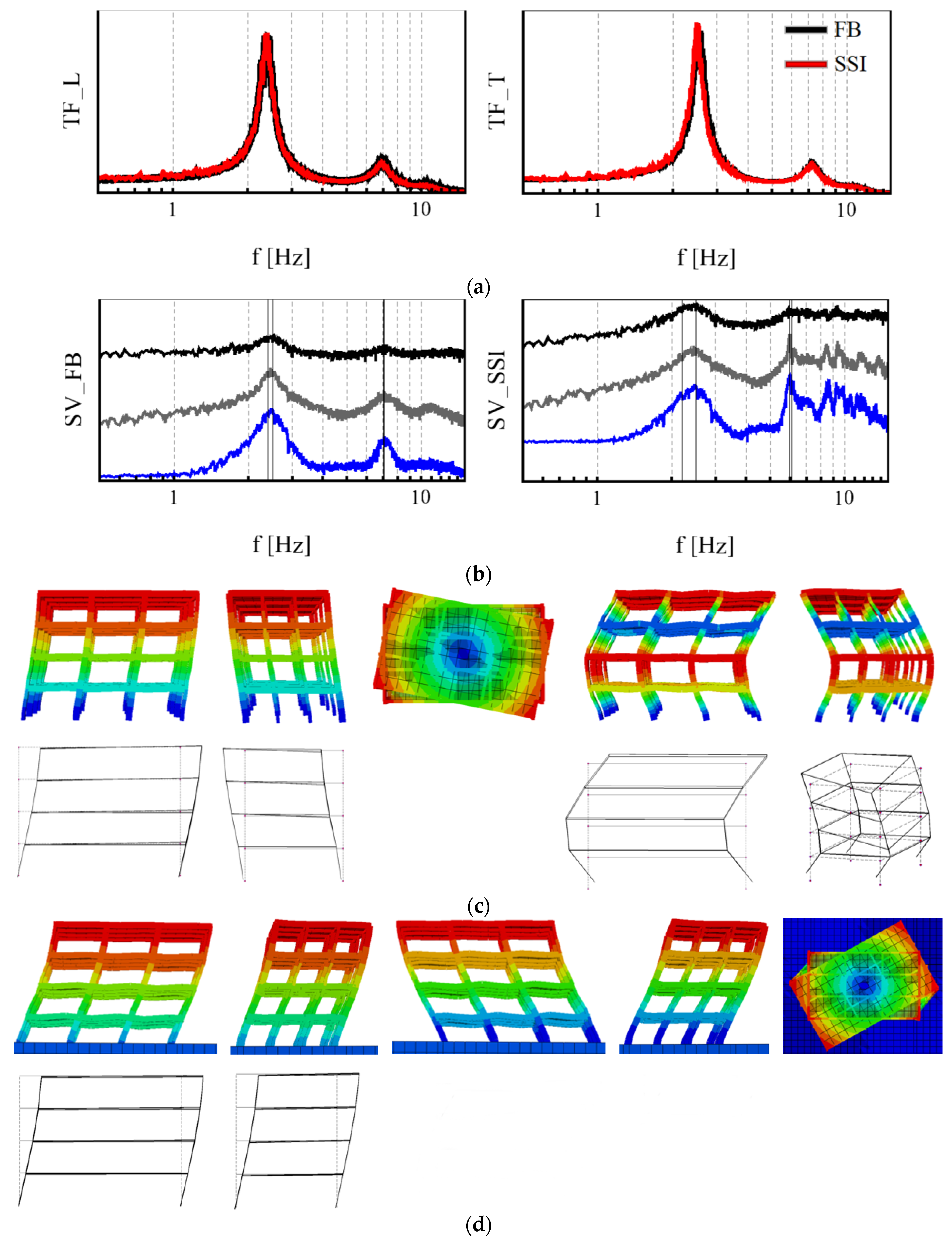
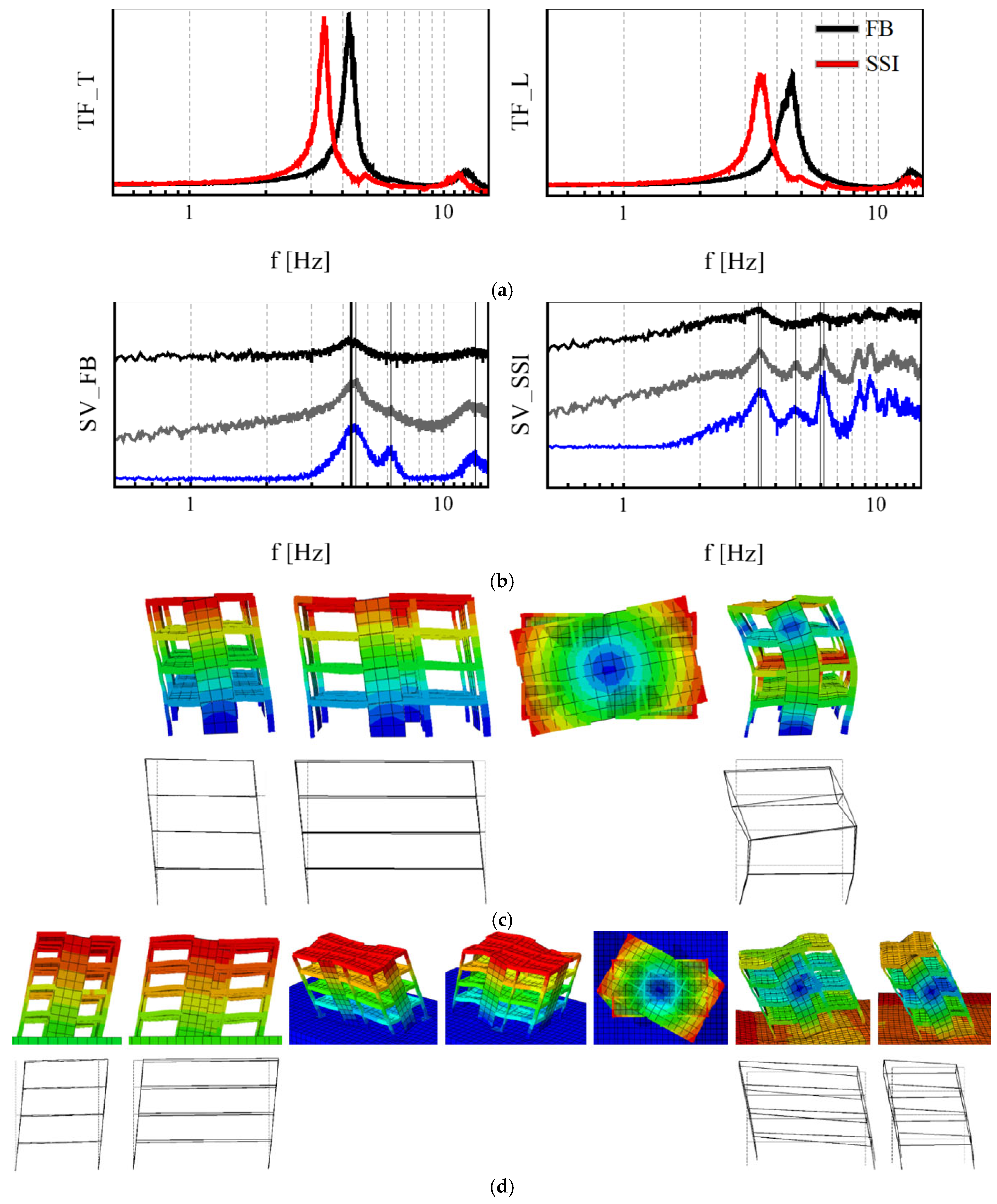
3.1. Frequency Domain Analysis
3.2. Rocking Estimation
4. Input Data
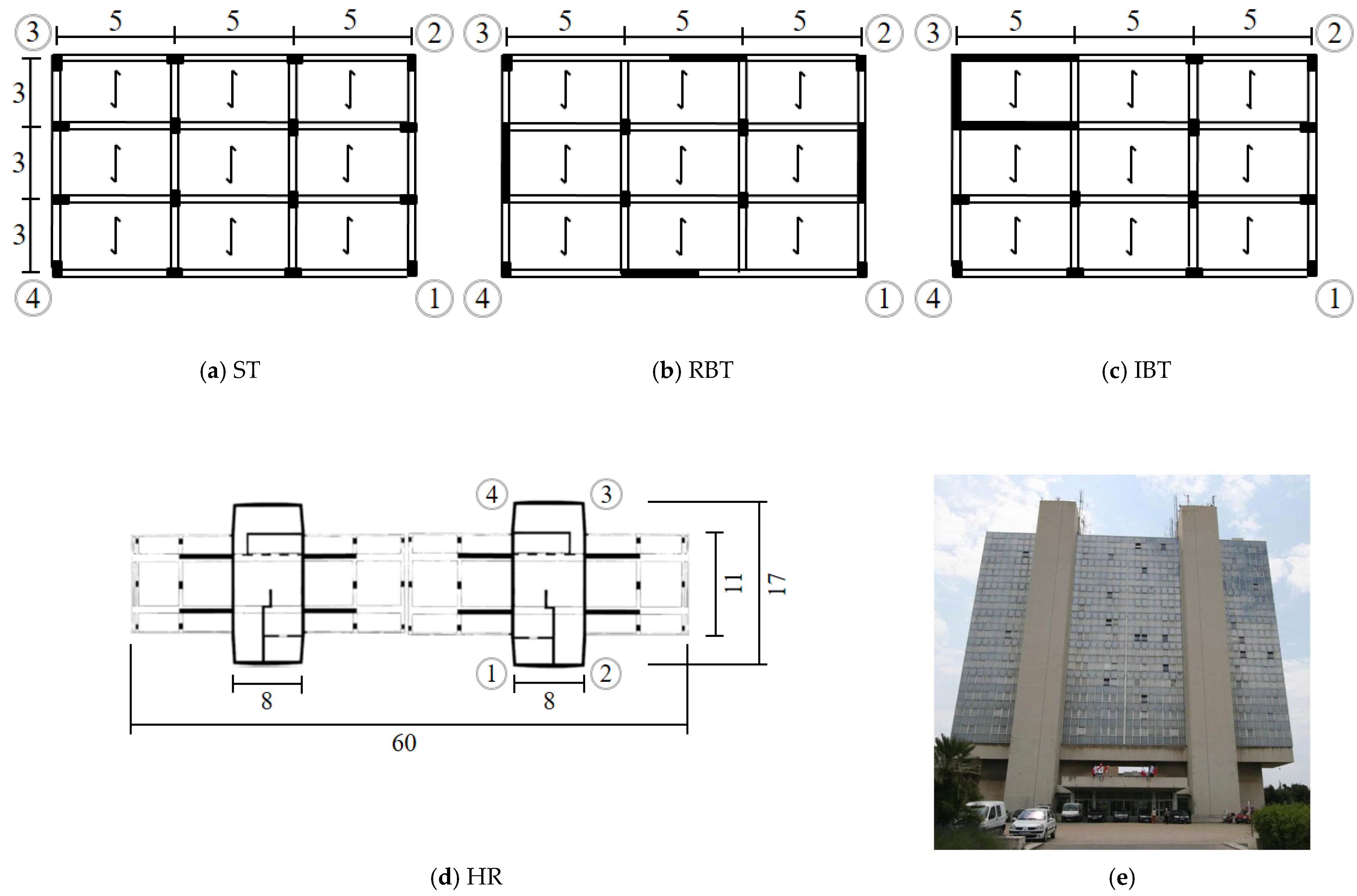
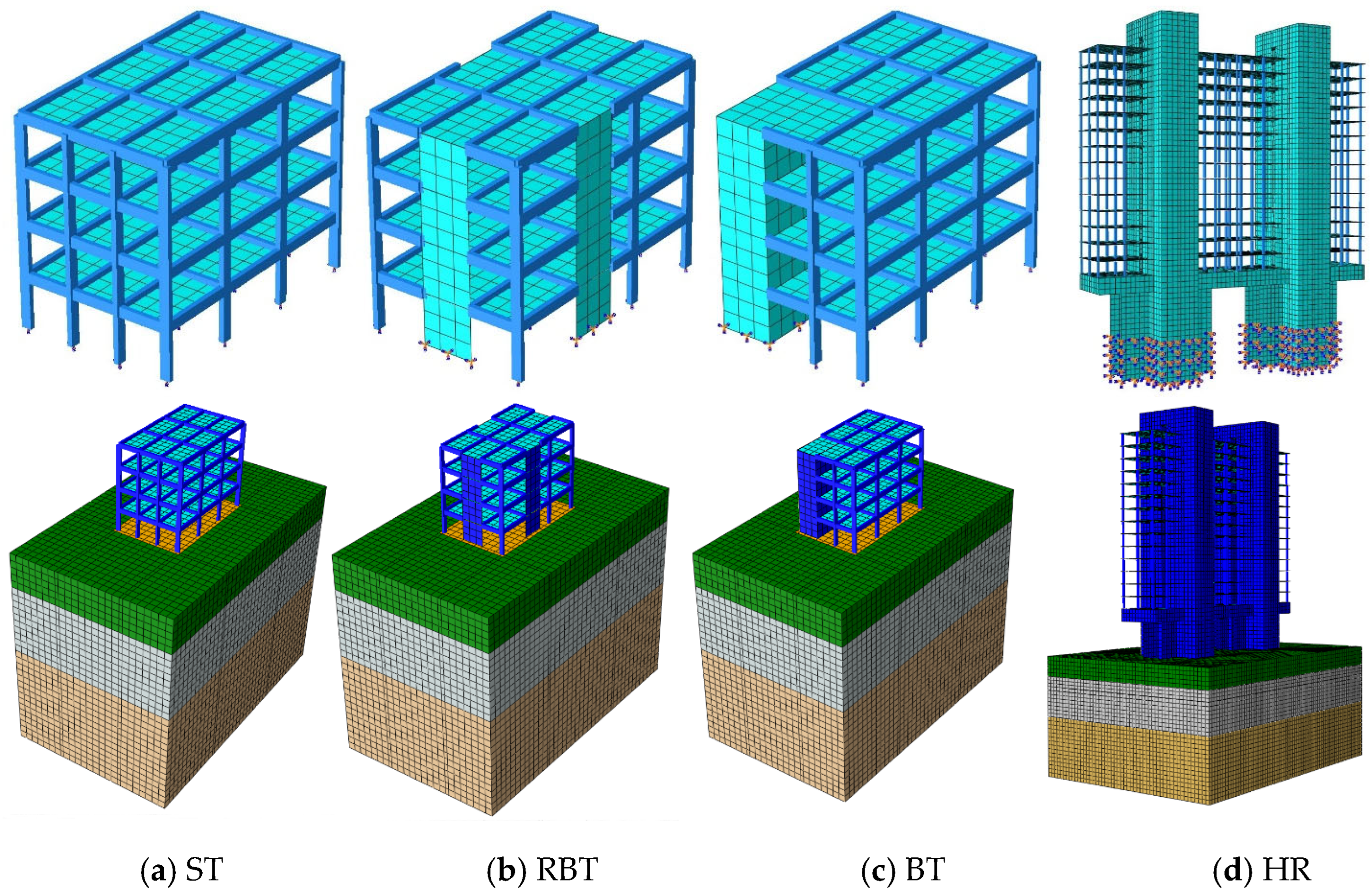
4.1. Buildings
4.2. Soil Profile
4.3. Synthetic White Noise and Recorded Seismic Loading
5. Identification of Building Dynamic Features
6. Rocking Motion Analysis Using Numerical Structural Response
7. Rocking Motion Analysis Using Recorded Structural Response
8. Conclusions
- The rocking ratio , detecting the phase shift of vertical displacement time history at the corners of the building base and indicating when rocking motion occurs for a specific frequency band;
- The rocking amplitude ratio , an amplitude criterion proposed to estimate the part of rocking motion on the whole horizontal motion at the top of the building, allowing the estimation of an expected rocking tendency;
- The rocking spectrum indicates the frequency bands in which the rocking motion is amplified because the first mode is not necessarily the only one affected by the swaying motion, and higher modes can also be affected.
Author Contributions
Funding
Data Availability Statement
Conflicts of Interest
Appendix A
Appendix A.1. Soil Domain
Appendix A.2. Building Structure
Appendix A.3. Mechanical Parameters of Building Structure and Loads
References
- Veletsos, A.S.; Meek, J.W. Dynamic behaviour of building-foundation systems. Earthq. Eng. Struct. Dyn. 1974, 3, 121–138. [Google Scholar] [CrossRef]
- Chopra, A.K.; Gutierrez, J.A. Earthquake response analysis of multistorey buildings including foundation interaction. Earthq. Eng. Struct. Dyn. 1974, 3, 65–77. [Google Scholar] [CrossRef]
- Jennings, P.C.; Bielak, J. Dynamics of building-soil interaction. Bull. Seismol. Soc. Am. 1973, 63, 9–48. [Google Scholar] [CrossRef]
- Stewart, J.P.; Seed, R.B.; Fenves, G.L. Seismic Soil-Structure Interaction in Buildings. II: Empirical Findings. J. Geotech. Geoenviron. Eng. 1999, 125, 38–48. [Google Scholar] [CrossRef] [Green Version]
- Stewart, J.P.; Fenves, G.L.; Seed, R.B. Seismic Soil-Structure Interaction in Buildings. I: Analytical Methods, J. Geotech. Geoenviron. Eng. 1999, 125, 26–37. [Google Scholar]
- Saez, E.; Lopez-Caballero, F.; Modaressi-Farahmand-Razavi, A. Effect of the inelastic dynamic soil-structure interaction on the seismic vulnerability assessment. Struct. Saf. 2011, 33, 51–63. [Google Scholar] [CrossRef]
- Dunand, F. Pertinence du Bruit de Fond Sismique pour la Caractérisation Dynamique et l’Aide au Diagnostique Sismique des Structures de Génie Civil. Ph.D. Thesis, Université Joseph Fourier, Grenoble, France, 2005. [Google Scholar]
- Hughes, T.J.R. The Finite Element Method—Linear Static and Dynamic Finite Element Analysis; Prentice Hall Englewood Cliff: Hoboken, NJ, USA, 1987; pp. 490–567. [Google Scholar]
- Konno, K.; Ohmachi, T. Ground-Motion Characteristics Estimated from Spectral Ratio between Horizontal and Vertical Components of Microtremor. Bull. Seismol. Soc. Am. 1998, 88, 228–241. [Google Scholar] [CrossRef]
- Brincker, R.; Zhang, L.; Andersen, P. Output-only modal analysis by frequency domain decomposition. Smart Mater. Struct. 2001, 10, 441–445. [Google Scholar] [CrossRef] [Green Version]
- Brincker, R.; Ventura, C. Introduction to Operational Modal Analysis; John Wiley & Sons: Hoboken, NJ, USA, 2015. [Google Scholar]
- Cole, H.A. On-Line Failure Detection and Damping Measurements of Aerospace Structures by Random Decrement Signature; NASA CR-2205; NASA: Washington, DC, USA, 1973; pp. 1–82. [Google Scholar]
- Rodrigues, J.; Brincker, R. Application of the Random Decrement Technique in Operational Modal Analysis. In Proceedings of the 1st International Operational Modal Analysis Conference, Copenhagen, Denmark, 26–27 April 2005; pp. 191–200. [Google Scholar]
- Lorenzo, G.W.F.; d’Avila, M.P.S.; Deschamps, A.; Bertrand, E.; Mercerat, E.D.; Foundotos, L.; Courboulex, F. Numerical and Empirical Simulation of Linear Elastic Seismic Response of a Building: The Case of Nice Prefecture. Earthq. Spectra 2018, 34, 169–196. [Google Scholar] [CrossRef]
- Fares, R.; d′Avila, M.P.S.; Deschamps, A. Response spectrum considering soil-structure interaction for buildings with shallow foundation. In Proceedings of the 16th European Conference on Earthquake Engineering, Thessaloniki, Greece, 18–21 June 2018. [Google Scholar]
- EN 1998-1:2004; Eurocode 8: Design of Structures for Earthquake Resistance—Part 1: General Rules, Seismic Actions and Rules for Buildings. CEN: Brussles, Belgium, 2003.
- Boore, D.M. Notes on Relating Density to Velocity for Use in Site Amplification Calculations. 2015. Available online: https://www.daveboore.com/daves_notes.html (accessed on 20 July 2022).
- Zienkiewicz, O.C.; Bicanic, N.; Shen, F.Q. Earthquake input definition and the trasmitting boundary conditions. In Advances in Computational Nonlinear Mechanics; International Centre for Mechanical Sciences, Doltsinis, I.S., Eds.; Springer: Vienna, Austria, 1989; pp. 109–138. [Google Scholar]
- Fares, R.; d’Avila, M.P.S.; Deschamps, A. Advantages and detriments of 1-Directional 3-Component wave propagation approach for Soil-Structure Interaction modeling. Procedia Eng. 2017, 199, 2426–2432. [Google Scholar] [CrossRef]
- Joyner, W.B.; Chen, A.T.F. Calculation of nonlinear ground response in earthquakes. Bull. Seismol. Soc. Am. 1975, 65, 1315–1336. [Google Scholar]
- Fares, R.; d’Avila, M.P.S.; Deschamps, A. Soil-structure interaction analysis using a 1DT-3C wave propagation model. Soil Dyn. Earthq. Eng. 2019, 120, 200–213. [Google Scholar] [CrossRef]
- Kaneko, T. On Timoshenko’s correction for shear in vibrating beams. J. Phys. D Appl. Phys. 1975, 8, 1927–1936. [Google Scholar] [CrossRef]
- Chopra, A.K. Dynamics of Structures: Theory and Applications to Earthquake Engineering; Prentice-Hall: Upper Saddle River, NJ, USA, 2001. [Google Scholar]


| Building | Floors | H | L | W | Foundation | Soil Area | ||
|---|---|---|---|---|---|---|---|---|
| (m) | (m) | (m) | (m × m) | (m × m) | ||||
| ST | 4 | 12 | 15 | 9 | 16 × 10 | 40 × 24 | 0.8 | 1.00 |
| RBT | 4 | 12 | 15 | 9 | 16 × 10 | 40 × 24 | 1.3 | 1.82 |
| IBT | 4 | 12 | 15 | 9 | 16 × 10 | 40 × 24 | 1.3 | 1.24 |
| HR | 20 | 60 | 17 | 8 | 56 × 24 | 70 × 50 | 7.5 | 0.56 |
| Depth | Thickness | vp | vs | |
|---|---|---|---|---|
| (m) | (m) | (kg/m3) | (m/s) | (m/s) |
| 5 | 5 | 1930 | 1330 | 200 |
| 10 | 10 | 1930 | 1400 | 240 |
| 30 | 15 | 1926.4 | 1500 | 300 |
| >30 | 2000 | 2449.5 | 1000 |
| FB | SSI | ||||||||||
|---|---|---|---|---|---|---|---|---|---|---|---|
| FE | TF | FDD | FE | TF | FDD | ||||||
| Bldg | Mode | Dir | f (Hz) | ε (%) | f (Hz) | f (Hz) | Dir | f (Hz) | ε (%) | f (Hz) | f (Hz) |
| 1 | TL | 2.40 | 83.5 | 2.4 | 2.4 | TL | 2.19 | 46.0 | 2.4 | 2.2 | |
| 2 | TT | 2.59 | 84.1 | 2.55 | 2.5 | TT | 2.23 | 55.8 | 2.5 | 2.5 | |
| ST | 3 | T | 2.98 | 0.0 | - | - | TL | 2.56 | 31.9 | - | - |
| 4 | TL2 | 7.50 | 10.4 | 6.9 | 7.0 | TT | 2.63 | 22.1 | - | - | |
| 5 | TT2 | 7.96 | 10.5 | 7.3 | 7.1 | T | 2.97 | 0.0 | - | - | |
| 6 | T | 9.22 | 0.0 | - | - | TL2 | 6.37 | 10.6 | 6.9 | 6.0 | |
| 7 | TT2 | 6.39 | 9.1 | 7.3 | 6.1 | ||||||
| 1 | TT | 4.36 | 71.1 + 4.4 | 4.25 | 4.3 | TT | 2.31 | 64.5 + 10.6 | 3.4 | 3.4 | |
| 2 | TL | 4.70 | 72.3 + 4.4 | 4.55 | 4.5 | TL | 3.22 | 65.0 + 10.7 | 3.45 | 3.5 | |
| RBT | 3 | T | 6.55 | 0.1 | - | 6.2 | TT | 3.44 | 2.5 | - | - |
| 4 | TT2 | 16.04 | 16.2 | 12.4 | 13.4 | TL | 3.60 | 2.1 | - | - | |
| 5 | TL2 | 19.26 | 13.5 | 13.5 | 16.5 | T | 4.99 | 0.0 | 4.8 | 4.8 | |
| 6 | TL2 | 6.40 | 10.0 | 6.2 | 6.0 | ||||||
| 7 | TT2 | 6.41 | 10.5 | 6.2 | 6.2 | ||||||
| 1 | TT + TL | 2.98 | 56.3 + 5.5 | 2.95 | 2.9 | TT + TL | 2.28 | 61.6 + 7.9 | 2.8 | 2.7 | |
| 2 | TL + TT | 7.23 | 58.2 + 12.6 | 6.8 | 6.7 | TL + TT | 2.31 | 67.6 + 8.7 | 2.8 | 2.8 | |
| IBT | 3 | TT2 | 9.22 | 4.5 | 9.1 | 8.5 | TT | 2.84 | 7.4 | - | 3.0 |
| 4 | T | 10.45 | 14.7 + 11.4 | 9.4 | TL | 3.94 | 1.7 | 3.9 | 3.9 | ||
| 5 | TT2 | 6.16 | 2.6 | 5.95 | 5.9 | ||||||
| 6 | TL2 | 6.42 | 9.8 | 6.8 | 6.1 | ||||||
| 1 | TT | 1.34 | 57.7 | 1.35 | 1.3 | TT | 0.97 | 7.2 | 1.0 | 0.96 | |
| 2 | TL | 1.48 | 63.1 | 1.45 | 1.5 | TL | 0.98 | 7.9 | 1.0 | 0.98 | |
| HR | 3 | T | 1.86 | 0.0 | - | - | T | 1.37 | 0.0 | - | - |
| 4 | TT2 | 6.19 | 18.4 | 5.90 | 5.1 | TT2 | 2.40 | 71.3 | 4.9 | 2.4 | |
| 5 | TL2 | 7.10 | 0.0 | 6.10 | 5.2 | TL2 | 2.42 | 70.6 | 5.3 | 2.5 |
| Earthquake | White Noise | |||
|---|---|---|---|---|
| Building | Dir. | Mode | RA (%) | RA (%) |
| ST | L | 1 | 0.6 | 0.55 |
| T | 2 | 0.0 | 0.00 | |
| RBT | L | 2 | 2.3 | 2.3 |
| T | 1 | 19.5 | 20.0 | |
| IBT | L | 2 | 19.0–6.7 | 4.1–0.1 |
| T | 1 | 28.5 | 25.0–20.6 | |
| HR | L | 2 | 0.8 | 0.3 |
| T | 1 | 39.8 | 43.0 |
Disclaimer/Publisher’s Note: The statements, opinions and data contained in all publications are solely those of the individual author(s) and contributor(s) and not of MDPI and/or the editor(s). MDPI and/or the editor(s) disclaim responsibility for any injury to people or property resulting from any ideas, methods, instructions or products referred to in the content. |
© 2023 by the authors. Licensee MDPI, Basel, Switzerland. This article is an open access article distributed under the terms and conditions of the Creative Commons Attribution (CC BY) license (https://creativecommons.org/licenses/by/4.0/).
Share and Cite
Rohmer, O.; Santisi d’Avila, M.P.; Bertrand, E.; Regnier, J. Rocking Motion Analysis Using Structural Identification Tools. Geotechnics 2023, 3, 601-623. https://doi.org/10.3390/geotechnics3030033
Rohmer O, Santisi d’Avila MP, Bertrand E, Regnier J. Rocking Motion Analysis Using Structural Identification Tools. Geotechnics. 2023; 3(3):601-623. https://doi.org/10.3390/geotechnics3030033
Chicago/Turabian StyleRohmer, Ophélie, Maria Paola Santisi d’Avila, Etienne Bertrand, and Julie Regnier. 2023. "Rocking Motion Analysis Using Structural Identification Tools" Geotechnics 3, no. 3: 601-623. https://doi.org/10.3390/geotechnics3030033
APA StyleRohmer, O., Santisi d’Avila, M. P., Bertrand, E., & Regnier, J. (2023). Rocking Motion Analysis Using Structural Identification Tools. Geotechnics, 3(3), 601-623. https://doi.org/10.3390/geotechnics3030033