Review

Investigating Sand Production Phenomena: An Appraisal of Past and Emerging Laboratory Experiments and Analytical Models

by
Kenneth Imo-Imo Israel Eshiet
and
Yong Sheng
*
Faculty of Science and Engineering, School of Architecture and the Built Environment, University of Wolverhampton, Wolverhampton WV1 1LY, UK
*
Author to whom correspondence should be addressed.
Geotechnics 2021, 1(2), 492-533; https://doi.org/10.3390/geotechnics1020023
Submission received: 19 October 2021 / Revised: 29 October 2021 / Accepted: 2 November 2021 / Published: 7 December 2021

Abstract

:
This paper provides an in-depth review of research developments on a common phenomenon in oil and gas exploration: sand production. Due to its significant impact to reservoir productivity and production efficiency, sand production has been widely researched in recent years. This paper focused on the review of historical progress in experimental and analytical studies which helped to understand the nature of the sanding mechanism and identify conditions that favour the process. Collation of the experimental data and analytical solutions and formulations enabled the authors to comment on effectiveness and also limitations of the existing experimental protocols and analytical models. Sand production models were then grouped into categories based on initiation of sanding, rate and amount of sanding as well as the failure criterion incorporated in their formulation so that it will be more convenient for future researchers to identify and adopt an appropriate model for their own research. The review also confirms that there are still some aspects of sand production requiring further investigation, and maybe a hybrid approach combining experimental, analytical and numerical methods could be the best solution for future explorations.

1. Introduction

The exploration and production of reservoirs for oil and gas is an age-long activity necessary to meet the global demand for energy. Global production of hydrocarbons has been on a steady increase [1] despite the campaign for alternative, green and sustainable energy sources and the clamour to reduce emission of greenhouse gases to combat adverse climate changes. There are claims of a direct correlation between consumption of fossil fuels and global warming, prompting an increase in efforts by leading governments to reduce the share of hydrocarbons in the global energy market.
The advent of new theories and concepts culminating in several innovations has led to a modest rise in the development of renewable and sustainable energy sources, which has, somewhat, altered the dynamics of the worldwide distribution of energy sources and their role in the world economy. This simply affirms the recognisable collective contribution of alternative energy sources. In spite of the increase in adoption of renewable and green energy sources, the average consumption of hydrocarbon-based fuels is still on the rise. At the end of 2019 the global supply and consumption of petroleum and liquid fuels was 100.66 and 100.90 million barrels per day respectively, indicating a rise in comparison to around 96.5 million barrels per day produced and consumed in 2016 [2]. There was a sharp slump in world consumption to about 85 million barrels per day as the effect of the COVID 19 pandemic became more widespread; nonetheless, this trend is currently reversed, and the amount of production and consumption has since accelerated. The forecast is that by 2022, the total world consumption will reach 101.31 million barrels per day [2]. Therefore, on average, the high demand for oil and gas has been consistent. This is reflected in the increasing exploitation of both conventional and unconventional reservoirs including those that are depleted. This implies a growing pressure on sandstone reservoirs as production schedules become more aggressive and an increasing presence of sand production problems during operations.
Sand production is a common phenomenon and is described as the movement of formation sand induced by fluid flow within reservoirs. This phenomenon impedes production efficiency and raises concerns about safety [3]. It is predominant in sandstone reservoirs, especially those that are unconsolidated or weakly consolidated [3]. The causes of sand production are multifaceted, but it is generally instigated when the rocks surrounding a wellbore perforation fail in such way that the drag forces from outflowing fluid are able to drive loose rock particles into the borehole. Sanding conditions are influenced by an array of factors that include the orientation, size and frequency of wellbore perforations; drawdown; reservoir depletion; strength properties of the rock; depth of production; pressure; characteristics of reservoir fluid, particle size and shape; water cut; shutdown/start-up frequency and size of bean-up [4].
The significance and large scale of the sand production problem is obvious when viewed in the context in which about seventy percent of global hydrocarbon reserves are present in unconsolidated reservoirs [5,6]. Unconsolidated and weakly consolidated reservoirs are prone to producing sand due to the relative ease at which the rock materials are eroded during the production cycle; hence, the problem is prevalent.
Paradoxically, although sand production hinders production efficiency, the phenomena can be used to boost reservoir productivity by enabling periodic sanding incorporated as one of the stages in the operation schedule [5]. To achieve this, it is imperative for conditions that influence sand production and their interplay to be controlled. This flip side means that sanding mechanisms can be deliberately triggered to enhance productivity of difficult reservoirs such as heavy oil fields [5,7,8]. Evidence of this is the increase of the sand-free flow rate by up to 44% after sanding has ceased [5,9].
Thus, the impact of sand production is considered as two-fold. In the downside scenario, it causes an influx of sand particles into the wellbore with dire consequences such as wellbore instability, abrasion of surface facilities (e.g., pipelines and valves) and well casing, damage to downhole equipment and pumps, accumulation of deposits in separators, and plugging of pipes and valves [4,5,10]. This devalues the well integrity and may eventually result in the failure of the wellbore. There will be a reduction in production time as well as the volume and quality of hydrocarbon produced. In addition, there will be a rise in the cost of disposal in the bid to meet health and safety regulations. The upside scenario is the accrued benefits associated with sand production. It can be harnessed to enhance well productivity and has been incorporated successfully in the recovery of heavy reservoirs through the implementation of the Cold Heavy Oil Production with Sand (CHOPS) technique to improve the rate of production beyond that possible with conventional methods [4,11].
Therefore, the relevance of sand production in oil and gas exploration cannot be overstated because of the sheer gravity of its impact on reservoir productivity and production efficiency. This article provides an insight into sand production as a prime area of interest in the petroleum industry. To this end, the subject of sand production is covered from a holistic perspective to meet sundry objectives. These are the following:
  • To highlight the salient and, more importantly, the non-salient issues associated with the phenomenon
  • To review the progress that has been made towards understanding the phenomenon
  • To identify and examine state-of-the-art experimental and analytical techniques and tools used to investigate the process
  • To track and assess past and current management and control strategies
  • To reveal the constraints and limitations of techniques and tools used to investigate the process
  • To proffer recommendations for better predictions, management and control strategies.
The second section focuses on rock failure and sanding mechanisms. This is necessary because the various investigations and models developed are fundamentally based on the understanding and interpretations of what are perceived to be the governing processes. The third section (Experimental Studies) covers historical and current developments of the experiments used to simulate and examine the sanding process. The fourth section (Analytical Modelling) is an overview and assessment of a broad spectrum of analytical models that simulate and analyse the sanding mechanism. A supplementary discourse is offered in Section 5 (Summary and Further Discussion), which highlights the constraints and limitations of the research tools and methods presented. These serve as a precursor for the identification of research gaps and potential areas for future studies.

2. Sanding Mechanism and Failure Criteria

An in-depth understanding of the causal factors and the sequence of events culminating in sand production is vital for accurate prediction, monitoring, control and management of the process. In the most simplistic terms, sand production happens when induced stresses exceed the reservoir rock in situ strength. The in-situ reservoir or formation rock strength is a function of factors such as the rock properties and overburdening and confining pressures. The most dominating factors affecting the rock strength are those associated with the natural cementation of the rock particles [12]. This is controlled by the bonding of cementitious materials, interparticle friction and fluid adhesion [13,14], which has a direct bearing on the mechanical integrity of the rock and the nature of its failure. This implies that rock formations with differing levels of competence will experience divergent modes of failure and hence different patterns of sanding mechanisms.
Using strength as a distinguishing criterion, sandstone formations can be split into three categories: unconsolidated, weak and competent [12]. On this premise, Al-Wad et al. [12] recognises two patterns of sanding process. In competent sandstone reservoirs, sanding is caused by shear failure, due to high shear stresses at the rock surface along the wellbore [12]. The detachment and movement of the rock grains, due to the drag forces, succeed this during reservoir fluid flow. In unconsolidated and weak sandstone reservoirs, sanding occurs when drag forces exerted by reservoir fluid flow overcome the binding cohesive forces between rock particles [12].
Some others [15] take an alternative view regarding the mechanisms responsible for sand production. For them, the mechanical integrity of the rock formation diminishes when there is both compressive and tensile failure. Compressive failure occurs when the compressive strength of the rock material around the wellbore perforation is exceeded by induced effective compressive stresses. This may be the consequence of stress redistribution induced during drilling and/or high pore pressure gradient/fluid flow. Tensile failure ensues when the tensile strength of the rock formation is overcome by tensile stresses exerted during reservoir fluid flow. Whereas compressive failure could be caused by fluid flow and/or other events, tensile failure is only instigated through fluid flow [15].
In addition to tensile and compressive failures, others such as Li et al. [13], Eshiet et al. [16], Eshiet and Sheng [8] and Nouri et al. [17] explicitly recognise the contributions of shear stresses and the role of shear failure in the sanding process. However, Li et al. [13] do not account for compressive failure but acknowledge the existence of a different form of failure, referred to as ‘bond failure’. This type of failure is more common in formations with weak cementation, where the bond strength governs the erosion process. The sanding event runs its course when the drag force exerted by fluid flow is greater than the bond strength [13,18]. This implies that there may be loss of mechanical integrity due to any one of shear, compressive, tensile or bond failure or a combination of them.
Since mechanical failure of rock material is considered a prerequisite for the occurrence of subsequent stages of the sanding process, it is necessary to break down the entire life span of an episode of sand production into phases. The number of phases and nature of events at each stage is dependent on the interpretation of the sequence of events and directly defines the way the process is modelled or idealised. Wu and Tan [15,19] break down the process into three consecutive steps. Initially, there is rock material failure at the vicinity of the wellbore perforation or openhole, resulting in the loss of mechanical integrity. Afterwards, there is grain detachment from the rock matrix by hydrodynamic forces, and finally, the loose particles move into and through the wellbore by the flow of reservoir fluids. Loss of mechanical integrity may be caused by an increase in intensity of stress concentrations during drilling works, the depletion of reservoir pressure, and drawdown. The sanding process may also be viewed as occurring in two consecutive stages [17,20]. First, there is mechanical degradation/loss of mechanical integrity with the possibility of rock disintegration, which is followed by the second stage involving the erosion or removal of materials that are disaggregated. Alternatively, the two–stage hypothesis is described as follows [21]: mechanical instability or loss of mechanical integrity caused by high stress concentrations, followed by hydro-mechanical/hydro-dynamic instability due to both internal and surface erosion caused by seepage or fluid flow drag forces. In the second stage, drag forces dislodge and transport loose particles.
The two mechanisms mentioned in the two-stage process are inter-related and coupled in such a way that creates a cycle of failure-production until a new equilibrium is attained where a stable cavity is formed [17]. During the course of sand production, the rock material fails and becomes disintegrated. Subsequently, as drag forces from fluid flow remove the failed material, this generates and redistributes the stresses within the area thereby propagating the failure zone and creating additional failed materials for production. As rock particles are flushed out, there is an increase in porosity and a redistribution of interparticle forces, which exacerbates the condition of the damaged zone.

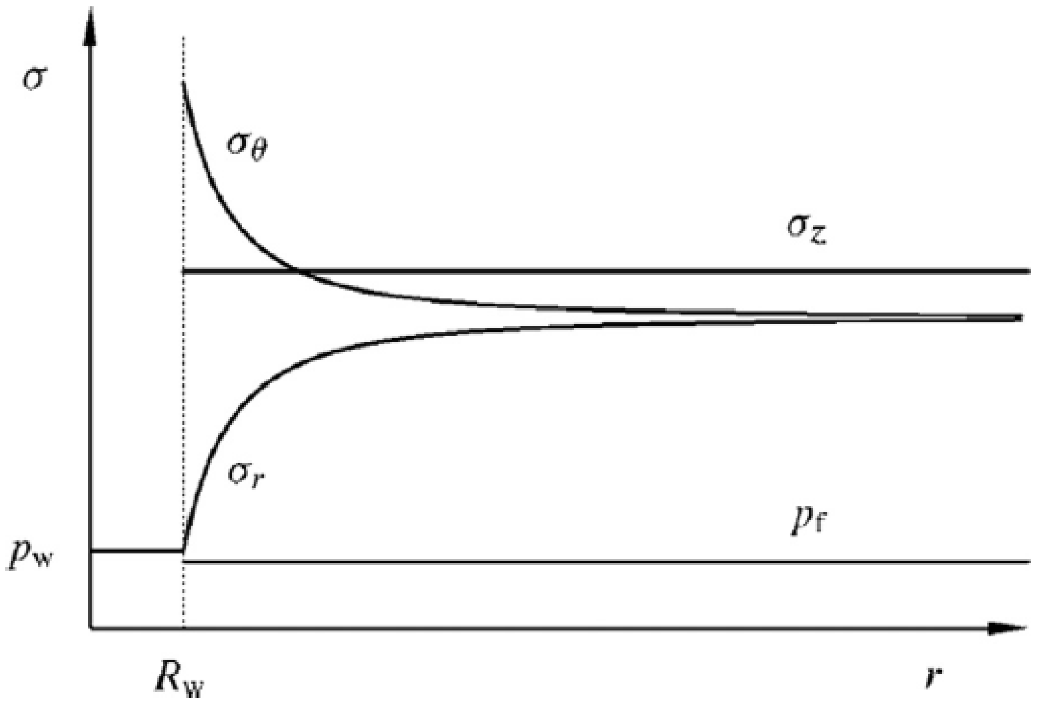
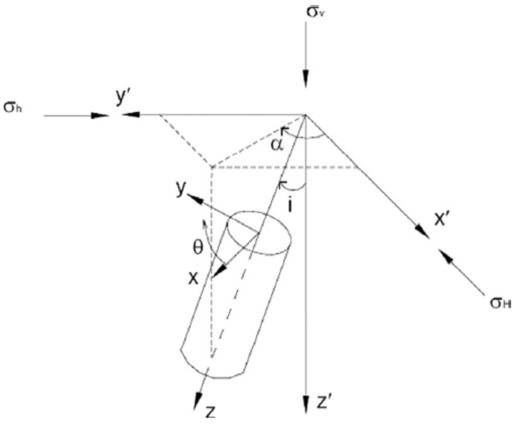
2.1. Stress Analysis

The geomechanical and hydrodynamic phenomena at the vicinity of wellbore openings are better understood by describing and representing the surrounding stresses. This is a common approach adopted in well stability and stress analyses. At the subsurface, in situ stresses are either naturally occurring or induced due to exploration. Both naturally occurring and induced stresses are bound to exist at the vicinity of the wellbore face as well as at far reach regions. Induced stresses tend to be generated by wellbore drilling and production operations. The stress distribution around the wellbore affects the material behaviour and processes governing fluid flow; therefore, it is imperative to understand their nature, including how they evolve.
Ideally, a stress tensor is a more comprehensive way of representing in situ stresses around a wellbore. Nonetheless, this can be simplified by using invariants such as the three principal stresses—i.e., the major, intermediate and minor principal stresses. For a vertical wellbore, this comprises two horizontal stresses a vertical stress. The effect of pore water pressure is used to depict the concept of effective stresses. During drilling and other exploration activities, different types and magnitude of stresses are developed, which changes the dynamics of the geological formation until a new equilibrium of stress system is established. At the first instance, the effect of this stress redistribution is more pronounced near the wellbore opening and to a lesser extent at the far-field regions. In some cases, far-field regions remain unaffected [22].
At subsurface levels, in situ stresses can be highly compressive. Overburden and lateral confining pressures generate vertical and horizontal stresses, respectively, while existing reservoir fluids contribute towards pore pressures. Drilling and excavation relieve the surrounding pressure causing stress concentrations at regions close to the wellbore face, which are initially linearly elastic [5,23]. These stress concentrations may engender shear (collapse) failure at the near-wellbore region. Shear failure happens when the pressure and density of the drilling fluid (mud) is below the critical values and can be prevented by using fluids with appropriate pressures and densities to establish the desired equilibrium. If the density and pressure of the drilling fluid are excessive, there is a tendency for loss of circulation at the near-wellbore region producing pressures that may exceed the sum of the minimum in situ compressive stress and the tensile strength of the formation rock, thereby triggering tensile failure. Tensile failure may also be instigated if the minimum effective stress becomes tensile and greater than the tensile strength of the formation rock [5,23].
The premise of a system consisting of three principal stress is generally acceptable and is adopted often in geo-mechanical analyses of stresses around circular holes. The magnitude and orientation of stresses can be influenced by conditions such as the topography near shallow underground areas and the presence of salt bodies [24]. Nonetheless, the system of stresses commonly embraced (especially for a vertically drilled wellbore) comprises one vertical principal stress, one maximum horizontal principal stress and one minimum horizontal principal stress [5,22,24,25]. In cylindrical coordinates, the horizontal components are termed the radial and tangential stresses, with the greater of the two regarded as the maximum horizontal principal stress.
Further discussion on stress analyses at the near-wellbore zone for vertical, inclined and horizontal wells is presented in, for example, Elyasi and Goshtasbi [26], Eshiet [5], Wang et al. [22], Zoback et al. [24], Risnes et al. [25] and Liao and Tsai [27]. Robust and comprehensive results can be achieved if the wellbore region is depicted in three dimensions and the analysis reliant on the theories of elasticity and plasticity. For instance, Risnes et al. [25] derives analytical stress solutions for elastic and plastic regions surrounding a wellbore in poorly consolidated formations. As a general caveat, the assumptions upon which these analyses are carried out should always be applicable to the scenario being considered. Some common assumptions are the following:
  • Fully saturated reservoir formation
  • Incompressibility of the reservoir and injected fluids
  • Steady flow and pressure conditions
  • Homogeneous and isotropic rock formation
  • Axial symmetry of wellbore area
  • Plane strain conditions
  • Three-dimensional stress orientations with vertical and horizontal principal stresses
  • Elastoplastic deformations.

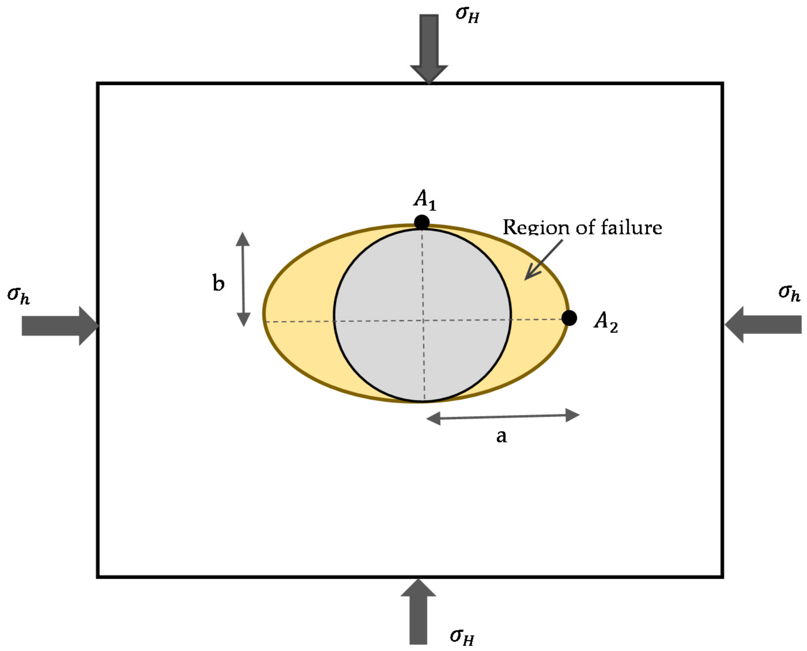
2.2. Tensile Failure

It is assumed that the removal of disintegrated material only occurs after rock material failure. There is potential for tensile failure when induced tensile stress is greater than the sum of the tensile strength of the rock and minimum compressive principal stress at a given position. According to the stress solution of an elastic rock material at a vertical wellbore opening, the minimum effective stress is the radial component and is equal to the pore pressure [25]. The maximum effective stress is the tangential component. Hence, for rocks that do not exhibit plasticity—brittle rocks—tensile failure will take place at the wellbore face if the combination of the compressive radial stress and rock tensile strength is overcome by induced stresses. If the radial stress is tensile, there may be tensile failure when it is equal to or exceeds the tensile strength of the rock [5].
For rocks that exhibit some degree of ductility, elastic stress solutions are not completely valid since the material will change from an elastic to a plastic state. The radial stress component will still be the smallest, but the largest stress component may be either vertical or tangential depending on the rock material characteristics and fluid flow conditions [25]. To determine the magnitude of these stresses it is imperative to define the boundary between the elastic and plastic regions. In general, tensile failure is instigated when the effective minimum tensile stress is equal or greater than the tensile strength of the rock [23].

2.3. Shear Failure

The elastic solution of stresses at the opening of a vertical wellbore indicates that the tangential and radial stresses are the maximum and minimum components, respectively. The effective radial stress is perpendicularly to the wellbore face and is zero at this point. On the other hand, the tangential stress is greatest at the same point [5,25]. Shear failure then depends on the difference between the maximum and minimum principal stress, which is greatest at the wellbore face. When plastic solutions are considered, the maximum principal stress is not necessarily tangential; it may be vertical [25]. Therefore, if the difference between the maximum and minimum principal stress is considered, a significant amount of shear stress can be generated at the wellbore face or at the boundary between the elastic and plastic zones, resulting in shear failure if the shear strength criterion of the rock material is satisfied. There are several shear-failure models, and some of these lead to results that are more conservative in comparison to others. Table 1 describes four typical shear failure models.
where:
S 0 = cohesive strength;
ϕ = angle of internal friction;
σ 1 = major principal stress;
σ 2 = intermediate principal stress;
σ 3 = minor principal stress;
I 1 = first invariant of the stress tensor;
J 2 = second invariant of the deviatoric stress tensor;
α d = material constant;
k d = material constant;
s = constant that depend on the initial state of the rock material;
m = constant that depend on the initial state of the rock material;
q ^ u c = uniaxial compressive strength;
τ o c t = octahedral shear stress;
σ m = effective normal stress.

2.4. Compressive Failure (Pore Collapse)

This is likely to occur when the formation rock is subjected to high confining stresses without any form of expansion, and the high compressive effective stresses exceed the yield strength of the rock causing irreversible plastic deformations [37,38]. This may lead to pore collapse, grain crushing and a drastic reduction in porosity and permeability. It may also occur in combination with shear. Compressive failure (pore collapse) happens when the effective compressive stress rises to a critical level due to excessive depletion of the reservoir pressure, usually during aggressive pumping schedules. Normally, it commences after the compressive stress surpasses the yield strength, and there is an increase in the rate of plastic volumetric strain. Pore collapse can take place at the vicinity of wellbore openings or perforations leading to the creation of a sand deposit and a proliferation of sand production [37].

3. Experimental Studies

Physical models are frequently used to mimic all or aspects of the sand production process. These are built either as laboratory or field set-ups where core samples are placed under quasi-field conditions to trigger sanding. For this purpose, it is necessary to obtain intact rock samples from target reservoir formations. The depth of petroleum reservoirs varies greatly, ranging from a few meters below the ground surface to a depth beyond 7000 m [39,40] and sometimes is difficult to retrieve large-scale cores from the required depth. Given the difficulty in extracting sufficient quantities of undisturbed natural cores, it is common practice to improvise using synthetic (artificial) cores [3,41,42,43,44]. Synthetic samples are complex to create since they must be representative of real reservoir rocks, especially when comparing their physical and mechanical properties and the dynamics of saturation and multi-phase characteristics. Creating such samples does not only require an in-depth understanding of their properties and behaviour at both microscopic and macroscopic scales; it is essential that the inter-relationship between the microscopic and macroscopic properties be established to an appropriate extent. One advantage of using synthetic rocks is the opportunity it provides to perform experiments on samples that are homogeneous with specific properties [3,44]. Natural rocks can be random in mechanical and physical properties, but at times, it is of the essence that tests be conducted using rock samples of specific and predefined properties.
Synthetic samples offer a great amount of flexibility making it possible to conduct tests on rocks with a wide range of properties. For instance, since sanding tends to be more predominant in weakly/unconsolidated rock formations, the degree of consolidation is a key property that can be emulated by altering the binder/cement content of the synthetic sample [3,43]. Artificial specimens can be constructed using simple materials such quartz sand, cement and water [3,45]. However, it is possible to create particles artificially, such as glass beads bonded by binders like epoxy resin mixed with acetone [46].
There is a growing number of laboratory experiments to simulate the sand production process [3,12,41,42,43,45,47,48,49,50,51]. These are fundamentally physical laboratory scale models constructed with either natural or artificial rock samples, placed under reservoir-like and sometimes wellbore-like conditions. The experimental set-up and sample configuration depend on the stage of the sanding process and the range of prevailing conditions to be examined. Reservoir erosion and sanding are mostly associated with wellbore instability during production, as formation fluids flow into the well or perforation cavity. Hence, to generate failure data from laboratory experiments, samples that are shaped as hollow cylinders or hollow prisms are commonly used. [47,48,52]. Hollow prism-shaped samples are ideal when it is necessary to apply anisotropic stress conditions. For instance, where there are disparities between the applied stresses—that is, the vertical stress and both lateral confining ones. Hollow cylinders are suitable for applying isotropic lateral stresses and are often used when the applied axial and lateral stresses are equal. The cavities in both hollow cylinder and prism specimens are usually not cased or supported, and fluid flow towards the cavity is instigated by applying a pressure gradient. The pressure gradient is established by ensuring the external pore pressure is greater than the internal (cavity) pore pressure [46,47,51].
The failure mechanisms of weakly consolidated or competent reservoir rocks (e.g., sandstone) can be investigated by placing thick-walled hollow or non-hollow specimens under prescribed stress and flow conditions [44]. Specimens are exposed to uniaxial or triaxial stresses that are meant to mimic reservoir stress distribution and material failure events. In some cases [48], rock material failure due to induced stresses is ignored, and the sanding process is studied with emphasis on the singular or combined effect of factors comprising confining pressures, pore pressure differentials and fluid flow rate. For unconsolidated rocks, it may not be necessary to establish material failure since it is assumed that they are non-cementitious and have negligible strength if the effects of confining pressures are neglected.
Perforation cavity models [3,53,54] and sand packs using hydrostatic physical models and the Hoek–Frankline cell [3,12,55,56] are some of the other ways in which rock specimens are set up for sand production experiments. In Yan et al. [3], Chin and Ramos [53] and Cook et al. [54], for example, perforation cavity models are made by, first, moulding the sample in form of a solid cylinder before drilling a hole at one end of the core to represent the downhole perforation channel. The specimen is mechanically loaded by applying axial and confining pressures, while an injection system enables a continuous inflow and outflow of fluid and seepage through the porous rock material; this causes a difference in pore pressure between the inner and outer perimeters of the core sample. The core is stressed gradually and isotropically by elevating the confining pressure until there is cavity failure.
Artificial samples must contain the correct particle size distribution (PSD). This means that the range of grain sizes and its distribution must be similar to the target reservoir rock. Younessi et al. [45] and Nouri et al. [44] used sand grains in the range 0.2–0.85 mm and 0.1–1 mm, respectively, to represent weakly consolidated/unconsolidated sandstones. Others such as Yan et al. [3] used median values (d50) of particles sizes and uniformity coefficients (CU) as alternative parameters to match. The uniformity coefficient is a ratio that numerically expresses the variation in particle sizes of a granular material. A value greater than 4.0 implies a well-graded material [57]. Another relevant PSD-based parameter is the coefficient of curvature/gradation (CC), which is a measure of gradation of the material and is normally applied in identifying poorly graded materials. A well-graded granular material has a CC value between 0.5 and 2.0 [58].
To bind natural (sand) or artificial particles (e.g., glass beads), they are mixed with binders like cement and epoxy resin [3,44,46]. Binders create the desired inter-particle bond, which contributes to the macroscopic mechanical strength properties of the specimen. The material composition/mix should be such that there is a considerably greater content of sand aggregates in comparison to both the binder and water. Nouri et al. [44] used a weight ratio of 0.11 and 1.25 for cement/sand and water/cement, respectively. This means 11 g of cement is mixed with every 100 g of sand and 13.75 g of water. The proportion of cement may be altered to either increase or reduce the bond strength and the representative degree of consolidation of the specimen. Obviously, a higher percentage of cement will raise the bond strength, which is shown by Yan et al. [3] to augment the uniaxial compressive strength, elastic modulus, friction angle and cohesion. Other factors like temperature and curing time also influence the mechanical properties of the synthetic rock [3]. Normally, curing is done under room temperature.
Where synthetic samples are used, it is imperative that the macro properties match those of real reservoir rocks. To this end, synthetic specimens should be calibrated, at least, in terms of key physical and mechanical properties including permeability, porosity, friction angle, Poisson ratio, elastic modulus, tensile strength, shear strength, compressive strength and uniaxial compressive strength. The calibration process is delicate and highly complex because of the interrelationship and/or unrelatedness of these properties, but it is a crucial part of the experiment
The experimental set-up is designed to enable the application of axial and confining pressures, fluid injection and a pore pressure gradient (Figure 1 and Figure 2). The rate of sand production is measured from the outflowing fluid containing produced sand. It is also possible to monitor deformations using cantilever displacement type transducers and linear variable differential transformers (LVDTs) [59,60], strain gauges or other forms of instrumentation. Confining stresses are applied on hollow cylindrical and/or perforation cavity specimens by placing them inside pressure cells, while top and bottom pistons/loading platens exert axial loads [51,59,60]. Actual values of axial and confining pressures depend on the well/perforation depth considered. For instance, using the relationship σ = ρ g h , an axial external stress of 13 MPa on a specimen with a bulk density of 2100 kg / m 2 can be used to represent a depth of 631 m.
Fluid is injected through designated inlets. For perforation cavity specimens, the fluid inlet (ports) could be the top or bottom of the specimen, depending on the vertical orientation of the specimen (Figure 1). If the perforation cavity is inverted (faces downwards), the fluid inlet is at the top of the specimen [10,59,60], and vice versa. In hollow cylinder specimens, fluid is passed laterally from the vertical sides to create a radial flow towards the opening at the centre; this is achieved using sleeves with fluid ports (Figure 2).
As an alternative to sleeves with fluid ports, a highly permeable granular material (e.g., gravel) can serve as a medium between the external surface of the specimen and the sleeve [51]. In this case, the fluid is passed through the packed and highly permeable granular material into the specimen (Figure 2b). The fluid injection rate is externally controlled; it determines the flow rate at the inlet and through the specimen, as well as the corresponding pore pressure. The flow rate and pore pressure gradient should be representative of field conditions. The flow pattern is either radial or axial. In accordance with the experimental set-up and the configuration of the specimen, the trajectory of fluid in hollow samples is controlled to enable radial flow geometry towards the cavity (centre) [51]. In perforation cavity specimens, flow is regulated such that it becomes axial with respect to the orientation of the hole [10,59,60].
Flow rates can be varied [10,43,51,59,60,61,62] and have been reported to be as high as 5 l/min [43]. There is a direct and proportional relationship between the flow rate and pressure drop, which means that a range of high flow rates will generate large pressure gradients with the upper and lower limits occurring at the outer (fluid inlet) and inner (cavity) boundaries, respectively. The inner cavity pressure may be kept atmospheric (i.e., 1 bar or 101 kPa).
The rate and amount of sand produced can be monitored using a transparent sand trap placed at the bottom of the entrapment. In addition, it is possible to use a sand detector—which functions according to the principle of ultrasonic Doppler velocimetry—to register acoustic reflections. This gives an indication of the particle size [59,60]. An equally effective arrangement is the use of sieves and weighing balances to collect and weigh the particles manually as they are being produced [44,55]. Alternatively, load cells positioned at the bottom of the sand trap automatically records the rate of sanding [62].
Another form of sand production experimental set-up involves the use of sand beds in the stead of cores [55,63]. The specimen is prepared by placing and compacting the required mix of materials in layers in a cell until the desired bulk density is attained. To generate drag forces, a vertical pore pressure gradient is created by increasing the pore pressure at the top of the sand bed, which instigates a downward fluid flow [55]. A sand collection entrapment (sandbag/container and weighing balance) placed at the bottom of the sand bed collects and records the rate of sand production. As another option, an imitation wellbore (a tube) is inserted at the centre of the sand bed, and a radial pressure gradient is used to establish fluid flow from the outer circumferential boundaries towards the centrally placed tube; this can be accomplished with an oedometer cell consisting of a cased hole through the middle [63]. In this case, the sanding rate monitoring device and instrumentation are more appropriate at the bottom outlet of the tube.
The mechanism of a centrifuge can be employed to generate field-like states tantamount to reservoir conditions (Figure 3 and Figure 4). If the cell containing the specimen is propped at the end of the centrifuge, the rotation of the centrifuge is capable of producing a radial inertial acceleration field similar but more powerful than Earth’s gravitational field [62]. The centrifuge model simulates field-like vertical stress distributions comprising a free upper surface that is unstressed and an increasing magnitude of stress with depth that is based on the density of the material and the strength of the gravitational acceleration field [62]. It is also possible to cause inward radial fluid flow from the lateral boundaries towards the inner tube through the action of centrifugal forces (Figure 3b) [62] The cell (sand bed) containing a centrally placed inner tube is secured within the centrifuge. Spinning the material mix at high speeds causes a radial and inward motion of the less dense substance–fluid–in the direction of the centrally placed tube.
Amongst other key factors, the accuracy of centrifuge physical models is dependent on the application of appropriate scaling laws [62,64]. These laws are derivatives of either dimensional analysis or relevant governing equations and are tailored towards magnifying properties such as acceleration and velocity to values greater than their counterpart prototype models but equivalent to real life conditions.
The duration of the sand production laboratory experiment generally depends on the time it takes for material failure and the transience of the sanding process. This could be as short as 2 h [60], where the loading process and the whole phenomenon of sand production are observed and recorded within the period. To imitate natural conditions, experimental loading is normally quasi-static, which means a gradual application of load resulting in slow structural deformation, infinitesimal strain rates and negligible inertia forces. Hence, the material remains in a constant state of equilibrium while being loaded, until material failure and sanding is initiated.
The sizes and shapes of test specimens vary but should be large enough to prevent speedy global collapse of the sample. They are either circular or cubic, with holes drilled at the centre to represent wellbores. The dimension of internal holes should minimise any sample boundary effect on cavity failure. The size of the hole influences the amount of sand produced; this is especially so in high stress conditions and in strong rocks. Under one or both of these conditions, large boreholes and perforations tend to produce more sand as compared with when their sizes are small [43]. Sand production is independent of hole size in low stress conditions and weak rocks. In other words, with respect to low strength rocks at low stress conditions, the process of sand production is less sensitive to hole size. This is an important factor to consider in deciding the dimensions of test specimens. A big specimen is generally preferred. Usually, there are constraints associated with components of the set-up, videlicet, sizes of the pressure cell, loading frame, sample core, etc. Ideally, the size of the inner hole (borehole or perforation) would be based on factors including the prevailing stress level, the size of the specimen, boundary effects and the material strength. Table 2 is a cross-section of specimen dimensions used in typical sand production experiments.

4. Analytical Modelling

It is often possible to represent subsurface phenomena mathematically, just like many other processes. This means there are governing equations that denote numerous forms of underground mechanisms and material behaviour. The sand production process is imputed to mechanisms associated with rock material behaviour, stress regimes, wellbore stability, fluid flow and erosion mechanisms. These do not operate in isolation; rather, they are interrelated in an intricate and complex manner. Each of these mechanisms are predominantly govern by several factors and can be mathematically described as systems, either independent or interlinked with one another. Governing equations of mathematically models describe the changes in variables with, for instance, time or space, and their interdependencies. However, it is imperative that these equations are solved quantitatively and/or qualitatively to achieve any meaningful scientific and engineering significance. Solutions may be derived analytically, numerically, statistically or empirically. This section presents a close inspection of mathematically models and the corresponding governing equations that describe specific key mechanisms of the sand production process. This is succeeded by an outline of various analytical solutions/models that predict and analyse the sanding process.
It is common practice to view sand production as a two-stage process involving several mechanisms. The first stage is the material failure and loss of mechanical integrity of rock at the vicinity of the wellbore or perforation tunnel, whilst the second stage involves the disintegration of the rock into loose grains and their transport towards and into the wellbore opening [17,20,21]. Initially, the two stages occur consecutively and are non-concurrent—i.e., material failure followed by hydrodynamic instability and erosion. Afterwards, there is a reciprocal inter-relationship between the two stages, with one influencing the action of the other. These processes are described mathematically through the relevant governing equations.

4.1. Stress at Wellbore Opening

Mathematically, it is possible to express the state of the initial and changing stress regimes that affect the strength and stability at and around the wellbore. Stresses around the wellbore face play an integral role in rock material response to induced conditions, and the corresponding sanding process. The maximum stress concentrations usually occur near the wellbore; this happens, in particular, at the face of the opening. In a linear poroelastic formation with no fluid flow and constant pore pressure, the maximum stress is tangential ( σ θ ) and the difference between the stresses is largest at the wellbore opening [25,35] (Figure 5). Therefore, wellbore failure and thus sand production are expected to commence at the opening.
Because rock material failure near the wellbore is determined by the prevalent stress state, it is necessary to compare the stresses generated with the rock strength via one or more rock failure criteria. Generally, the stress solution at the face of a deviated wellbore (Figure 6) in cylindrical coordinates is given as [35]
σ z = σ z o υ 2 σ x o σ y o c o s 2 θ + 4 τ x y o s i n 2 θ + 2 η P o P f
σ θ = σ x o + σ y o 2 σ x o σ y o c o s 2 θ 4 τ x y o s i n 2 θ P w + 2 η P o P f
σ r = P w
τ θ z = 2 τ x z o s i n θ + τ y z o c o s θ
τ r θ = 0
τ r z = 0
where,
η = α 1 2 υ 2 1 υ
σ z o = σ H c o s 2 φ + σ h s i n 2 φ s i n 2 i + σ v c o s 2 i
σ x o = σ H c o s 2 φ + σ h s i n 2 φ c o s 2 i + σ v s i n 2 i
σ y o = σ H s i n 2 φ + σ h c o s 2 φ
τ x y o = 0.5 σ h σ H s i n 2 φ c o s i
τ y z o = 0.5 σ h σ H s i n 2 φ s i n i
τ x z o = 0.5 σ H c o s 2 φ + σ h s i n 2 φ σ v s i n 2 i
where,
σ z = Axial stress in (cylindrical coordinates);
σ θ = Tangential stress (cylindrical coordinates);
σ r = Radial stress (cylindrical coordinates);
τ θ z , τ r θ , τ r z = Shear stresses at the wellbore face;
σ x o ,   σ y o ,   σ z o = In situ normal stresses in the x, y, z coordinate system;
τ x y o , τ y z o , τ x z o = In situ shear stresses in the x, y, z coordinate system;
σ z , σ H , σ h = Vertical and horizontal in situ stresses;
υ = Poisson ratio;
η = Poroelastic stress coefficient;
P w = Wellbore pressure;
P o = Pore pressure at the wellbore;
P f = Pore pressure at far field region;
θ = Angle of rotation about the z axis referenced from the x axis;
α = Biot’s coefficient;
φ = Angle of rotation about the z’ axis referenced from the x’ axis;
i = Angle of rotation about the y’ axis referenced from the z’ axis.
If the wellbore is vertical, the angle of rotation about the z’ axis, i , is zero. Then the x-axis can be reoriented to match the x’-axis, which is in the same direction as the major principal stress ( σ H ), so that α = 0, x ,   =   x , y ,   =   y and z ,   =   z . The in-situ stresses reduce to
σ x o = σ H
σ y o = σ h
σ z o = σ v
τ x y o = τ y z o = τ x z o
Equation (6a–f) becomes
σ z = σ v 2 υ σ H σ h c o s 2 θ + 2 η P o P f
σ θ = σ H + σ h 2 σ H σ h c o s 2 θ P w + 2 η P o P f
σ r = P w
τ θ z = 0
Thus, for any set values of in situ stresses, the maximum stresses at the wall of a vertical wellbore occur where θ = ± 90 ° [35]. Equation (18a–d) changes to
σ z = σ v + 2 υ σ H σ h + 2 η P o P f
σ θ = 3 σ H σ h P w + 2 η P o P f
σ r = P w
τ θ z = τ r θ = τ r z = 0

4.2. Governing Equations

The choice of existing and derived governing equations depends on the range of relevant phenomena considered and the modelling approach. Typically, the following are considered:
  • The mass balance (continuity) equations for the different phases of the saturated porous material flow, comprising the solid, fluidised and liquid phases
  • Equations for fluid through porous media
  • Equations for permeability and porosity alteration
  • Constitutive laws describing the poro-elastoplastic mechanical behaviour of the rock
  • Constitutive laws describing the onset and/or rate of erosion of the solid mass
  • Sanding criteria.
A well-established approach—proposed by Papamichos and Vardoulakis[70], Papamichos and Stavropoulou [71] and Stavropoulou et al. [72]—for simulating sand production is to consider an erodible and saturated rock material subjected to both stresses and fluid flow as characterised by (a) the poro-mechanical behaviour of the fluid-filled porous rock and (b) the erosion of the solid matrix. This allows the poro-mechanical behaviour of the fluid-filled porous rock to be defined by equations of poro-elastoplasticity, while the equations of solid erosion define the erosion behaviour of the matrix. Poro-elastoplastic processes are described by equations for stress equilibrium, fluid flow continuity, Darcy’s flow and constitutive laws for the porous material. Steady-state fluid flow conditions are assumed for rocks (e.g., sandstone) with high permeability and are subjected to slow rates of loading. Under this state, the following equations apply [70,71].
Stress equilibrium:
σ i j , j = 0 ;   ( where   σ i j = σ j i )
Continuity of fluid flow:
q i , i = 0
Flow though porous media (Darcy’s law):
q i = k η P , i
Constitutive laws for the porous material [70,71]:
d σ i j = C i j k l e p d ε k l + α d p δ i j C i j p o r o d ϕ
where,
σ i j = Total stresses;
d σ i j = Stress increments;
C i j k l e p = Tangent elasto-plastic stiffness matrix;
d ε k l = Strain increments;
α = Biot’s coefficient for effective stress;
p = Pore pressure;
δ i j = Kronecker delta;
C i j p o r o = Tangent elasto-plastic porosity matrix;
ϕ = Porosity.
The erosion of the solid matrix is described by the following equations.
Mass balance equations for solid phase (Continuity equation):
m ˙ ρ s = ϕ t
Mass balance equations for fluidised solid phase (Continuity equation for fluidised particles):
m ˙ ρ s = c ϕ t + c q i , i
Permeability law (based on the classical Kozeny–Carman equation):
k = k o ρ ¯ ϕ 3 1 ϕ 2
Constitutive law for the rate of generation of eroded solid mass [71]:
m ˙ ρ s = λ 1 ϕ c q i q i
where,
m ˙ = Rate of eroded mass generation;
ρ s = Density of solid particles;
ρ ¯ = Density of mixture of fluid and solids;
t = Time;
c = transport concentration of fluidised solids;
q i = Fluid flux;
k o = Permeability parameter;
λ = Sand production coefficient.

4.3. Analytical Models

Analytical solutions, like other forms of models, are based upon what is envisage as the process and criterion for sanding. In many predictions, the onset of the sanding process coincides with rock material failure. Thus, sanding is attributed to the shear, tensile or compressive failure of the rock, occurring individually or in combination. In this approach, the emphasis is mainly on determining the stress evolution at the areas prone to failure (usually the near the wellbore opening) and then choosing or deriving representative rock material failure models. Expressions of stresses at the failure zones are incorporated in material failure models to establish analytical solutions of sand production criteria. Simply put, analytical sanding onset/production models are constructed by the use of poroelasticity and/or poroelastoplasticity to derive the relevant stress distributions at the well cavity and then by applying these stress expressions in a suitable failure criterion [47]. This form of simulation is presented by Yi [73], Al-Shaaibi et al. [35], Gholami et al. [74], Hayavi and Abdideh [75], Jianguang and Chuanliang [76], Li et al. [13], Papamichos [47], Papamichos and Furuic [77], Shabdirova et al. [14] and many others.

4.3.1. Shear Induced Sanding Prediction Models

Yi [73] developed two types of analytical models to predict the initiation of sanding production on the assumption that the rock is homogeneous, isotropic, linearly elastic and perfectly plastic, satisfies the Mohr–Coulomb failure criterion, deforms under plane strain condition and is subjected to axisymmetric external stresses. The first model assumes the rock material can fail in shear while still being elastic. A poroelastic analytical solution can then be developed whereby the tangential and radial stresses at the wellbore surface, which are the maximum and minimum stresses respectively, are incorporated in the Mohr–Coulomb failure criterion to predict the initiation of sand production. The elastic stress distribution (maximum and minimum stress) at the wellbore surface is given as [73]
σ θ , = 2 σ h t α b 1 2 υ 1 υ P ¯ t 1 + α b υ 1 υ P w t
σ r , = 1 α b P w t
A rearranged form of the Mohr–Coulomb criterion is
σ θ , σ r , 2 = σ θ , + σ r , 2 s i n ϕ f + C 0 c o s ϕ f
Based on the above stress distribution and Mohr–Coulomb criterion, the poroelastic analytical model for the onset of sand production at shear failure is
1 α b 1 + s i n ϕ f 1 s i n ϕ f + 1 + α b υ 1 υ P w t = 2 σ h t α b 1 2 υ 1 υ P ¯ t 2 C 0 c o s ϕ f 1 s i n ϕ f
If C 1 = 2 C 0 c o s ϕ f 1 s i n ϕ f , Equation (34) is simplified to a dimensionless form.
1 α b 1 + s i n ϕ f 1 s i n ϕ f + 1 + α b υ 1 υ P w t C 1 = 2 σ h t C 1 α b 1 2 υ 1 υ P ¯ t C 1 1
If Biot’s constant is 1, this is further simplified to
P w t C 1 = 1 υ 2 σ h t C 1 1 2 υ 1 υ P ¯ t C 1 1
Sanding is initiated when the bottomhole pressure, P w , is insufficient such that the left-hand side of the Equation (36) is less than the right-hand side.
where,
α b = Biot’s constant;
ϕ f = angle of internal friction;
P w = bottom hole flow pressure (psi);
P ¯ = average reservoir pressure (psi);
C 0 = cohesive strength (psi).
The above sanding criterion is based on the premise that the near cavity region fails in shear and sanding is initiated when this occurs. However, it is possible that the sand particles will still remain immobile despite shear failure and are dislodged only if flow drag forces are sufficiently large to displace the sand particles that failed in shear. Hence, a complimentary sand production criterion is necessary.
Yi’s second model [73] is an approach based on a poroelastoplastic stress solution coupled with a tensile failure criterion. It was suggested by Weingarten and Perkins [78]. This modelled is applicable to the condition when the failed zone is no longer elastic but plastic.
The poroelastoplastic stress solution is [73]
σ r , = α b r m R w r p r , t r r m d r + C h c r m C o c o t ϕ f
σ θ , = α b q r m R w r p r , t r r m d r + C h c q r m C o c o t ϕ f
m = 2 s i n ϕ f 1 s i n ϕ f
q = 1 + s i n ϕ f 1 s i n ϕ f
C h c = C o c o t ϕ f + 1 α b P w t R w m
Assuming the rock tensile strength in its disintegrated condition is negligible, the sanding criterion is expressed as [73]
d σ r , d r r = R w = 0
Combining Equations (37) and (42) gives
α b p r , t r r = R w = 2 s i n ϕ f 1 s i n ϕ f C o c o t ϕ f + 1 α b P w t R w
If Biot’s constant is 1, this is further simplified to
p r , t r r = R w = C 1 R w
Sanding is initiated when the pore fluid pressure gradient exceeds a threshold value given by C 1 R w . In other words, sanding occurs when the left-hand side of Equation (44) is greater than its right-hand side.
where,
r = radial co-ordinate (ft);
R w = radius of cavity (wellbore, perforation tunnel) (ft);
p = pore fluid pressure (psi).
For cases where in situ stresses acting around a well cavity are axisymmetrical (anisotropic), Yi [73] derived a Mohr–Coulomb shear failure induced sand production criterion, given as
1 α b 1 + s i n ϕ f 1 s i n ϕ f + α b υ 1 υ + 1 P w t = 3 σ H t σ h t α b 1 2 υ 1 υ P ¯ t 2 C 0 c o s ϕ f 1 s i n ϕ f
where, σ H and σ h is the maximum and minimum horizontal stress respectively, and σ H σ h .
If C 1 = 2 C 0 c o s ϕ f 1 s i n ϕ f , Equation (45) is simplified to a dimensionless form.
1 α b 1 + s i n ϕ f 1 s i n ϕ f + α b υ 1 υ + 1 P w t C 1 = 3 σ H t C 1 σ h t C 1 α b 1 2 υ 1 υ P ¯ t C 1 1
Assuming Biot’s constant is 1, Equation (45) becomes
P w t C 1 = 1 υ 3 σ h t C 1 σ h t C 1 1 2 υ 1 υ P ¯ t C 1 1
Sanding is initiated when the left-hand side of the Equation (46) is less than the right-hand side.
Using a broadly similar approach as Yi [73], Papamichos [47] proposed and compared four sand production analytical models based on the following rock failure criteria: Mohr–Coulomb, simplified Mohr–Coulomb, von Mises and Drucker Prager. For better predictions, the failure criteria were not calibrated using conventional uniaxial/triaxial compression tests; rather, they were calibrated using hole failure data from tests on hollow cylinder and hollow prism specimens. Hollow prismatic cubes permit the application of full anisotropic stress conditions. The approach used by Papamichos [47] is analogous to those adopted in other sanding onset analytical models but different because the proposed models are calibrated on failure data from hollow cylinder/prism laboratory tests. These hollow specimens do not just have the same geometry as what is obtainable in the field, they allow the effect of plasticity during straining to be incorporated.
Yi [73] and Papamichos [47] do not consider material anisotropy, yet an elaborate way of integrating stress anisotropy is given by Papamichos [47], where stress ratios are introduced to account for both axial stress anisotropy (axial stress/major lateral stress) and lateral stress anisotropy (minor lateral stress/major lateral stress). The cavity failure/sanding onset criterion for the four rock failure criteria as derived by Papamichos [47] is summarised in Table 3. A comparison of shear failure-based analytical models in a manner akin to that shown by Papamichos [47] is presented by Al-Shaaibi et al. [35], where onset of sanding is predicted using linear poroelastic formulations that are based upon either the Mogi–Coulomb or the Mohr–Coulomb failure criterion (Table 4). The models calculate the critical wellbore pressure and can be applied to trace the optimal well path, where the propensity for sanding is minimal. Sanding is initiated at values below the critical wellbore pressure.
The major difference between the models (i.e., Mohr–Coulomb failure-based models) by Papamichos [47] and Al-Shaaibi et al. [35] is drawn mainly from the variances in assumed initial and boundary conditions and the way in which the stress solutions and the material failure criteria are expressed. As an example, Papamichos [47] considers the initial radial stress at the wellbore vicinity as the minor principal stress and equal to zero (i.e., σ 3 = σ r i = 0 ), whereas the value of the radial stress given by Al-Shaaibi et al. [35] is equated to the internal wellbore pressure ( σ 3 = σ r i = P w ). Papamichos [47] models are also calibrated against hollow cylinder/prism tests. Notwithstanding, both sets of models are hinged on linear poroelastic constitutive laws. The Mogi–Coulomb failure criterion embeds the intermediate principal stress. Hence, the comparison of different material failure criteria provides an opportunity to assess the influence of the intermediate principal stress, which is normally ignored. Al-Shaaibi et al. [35] show that there is an excess in the estimation of the sanding pressure when the model neglects the intermediate principal stress. This produces conservative results that include an increase in the predicted amount of sanding beyond what is obtainable in reality. The intermediate stress affects the evaluation of the rock strength behaviour whilst underplaying the contribution of Biot’s coefficient in sand production models.
where:
k , k 1   = material strength parameters;
σ s = isotropic loading hole failure stress;
σ c = equivalent stress at the cavity;
η B = poroelastic constant;
K r = lateral anisotropy (minor lateral stress/major lateral stress);
K z = axial anisotropy (axial stress/major lateral stress);
K p = ratio of pore pressure difference to lateral stress (pore pressure difference/major lateral stress);
I 1 = first stress invariant of the stress tensor;
J 2 = second stress invariant of the stress deviator tensor;
σ Z = applied external axial stress;
σ R e = applied external major lateral stress;
σ r e = applied external minor lateral stress;
σ m , 2 = effective normal stress;
τ o c t = octahedral shear stress;
P w = internal wellbore pressure;
P f = pore pressure at wellbore wall;
P f 0 = pore pressure at far field;
η = poroelastic stress coefficient;
β = angle of failure.
While it is imperative to ascertain the conditions that enable the onset of sanding, it is equally important to predict the rate and amount of sanding over time. Estimates of the volume of sanding occurring within a given period are a strong indicator of the severity of the erosion as it progresses. There are several models that compute the mass/volume of sanding. Some of these are reliant on the action of the flowing fluid drag force on an already disintegrated rock mass and the presumption of a state of material that is unconsolidated and failed in tension [79,80,81]. A number of models acknowledge the prerequisite condition for the rock material to fail in shear but still adopt the principle of critical fluid and grain flow to fully fulfil the requirement for sand production [82]. Other models such as those by Shabdirova et al. [14] and Gholami et al. [74] are correlated with the shearing behaviour of the rock material, whereby sanding is deemed to be a direct offshoot of shear failure.
The model by Geilikman and Dusseault [82] (Equation (54a–f)) includes an explicit and direct relationship linking the span of the yield (plastic) region with the cumulative amount of sand produced. It is built on the premise of a yield condition described by the Mohr–Coulomb criterion, and there is a synchrony between the commencement of the plastic regime and the ability of the granular material to flow frictionally once yield is attained. This suggests that when the material yields, it becomes prone to frictional flow. The model recognises the role of solids and fluid velocity and the precondition that must be met—i.e., the wellbore fluid pressure falling below a critical value—in order to instigate the fulfilment of the yield criterion, thereby generating a yield zone. The initial condition is defined by the intact rock that surrounds the wellbore and is not yielded. If the wellbore pressure is slowly reduced to a threshold value, the yield condition will be satisfied. Further reduction in the wellbore pressure will lead to a growth of the plastic zone, propagating outwardly away from the wellbore.
q s = 1 n y Q 2 c 1 ϕ λ σ r r P y r r λ r w λ r λ 2 π n y k y 1 + b μ
q s = d S c d t
S c t = π n y n i R 2 r w 2
b = n i 1 n i
λ = 2 ϕ 1 ϕ
where,
S c = cumulative sand produced per unit length of the wellbore;
q s = volumetric discharge rate of sand produced;
Q = fluid + particle volumetric discharge per unit length of the wellbore;
n y = porosity of yielded region;
n i = porosity of intact region;
c = cohesion;
ϕ = coefficient of friction;
λ = parameter that is a function of the friction coefficient;
σ r = radial stress;
P y = fluid pressure at yielded region;
k y = permeability of yielded region;
μ = fluid viscosity;
r = radius measured from the centre of the wellbore;
r w = wellbore radius;
R = radius of yielded region;
b = coefficient that is related to porosity.
Shabdirova et al. [14] somewhat draws a parallel with Geilikman and Dusseault [82] by equating the volume of the plastic region of the rock material that has failed in shear with the volume of sand produced. As the stresses around a wellbore increase, the region will degenerate from an elastic to a plastic state after shear failure [25,83]. This creates a plastic zone that surrounds the wellbore [10,25,83,84]. Initially, the shape of this plastic region is assumed circular, aligning with the cross-sectional geometry of the wellbore. Thenceforth, there is a tendency for the shape of the plastic region to evolve towards an elliptical cross-section while expanding away from the periphery of the wellbore wall. It is assumed that the shape of the evolving plastic region does not change along the wellbore axis.
Most analytical models are built presupposing that the shape of the well/perforation cavity is not altered despite shear failure. Progressive changes in the wellbore geometry as it deforms affect the local stress distribution, with a possible knock-on bearing on the accuracy of predictions of analytical sand production models. Wellbores are usually circular in shape; however, there is a tendency for the geometry to become elliptical due to increasing stress concentrations and shear failure during drilling and production. It is generally accepted that the rock material surrounding a wellbore cavity changes from an elastic to a plastic state following shear failure. Shear failure occurs when the peak tangential stress exceeds a threshold value. Thus, the type of material failure model adopted plays a key role in defining the occurrence and transformation of the plastic zone. In addition, the solutions that describe the stress distributions around the wellbore cavity and the far field regions contribute towards the general state of the material around the wellbore. Some models are built upon stress solutions based on poro-elastic constitutive laws, while others are linked to their poro-elastoplastic counterparts. The configuration (e.g., shape and geometry) and the material of the wellbore wall also determine the nature of stress distribution as well as the failure mechanisms. Stress distributions around open wellbores differ from those concomitants with cased and perforated wellbores [14]. Obviously, these affect the failure mechanism. In cased and perforated wells, the initial sand produced is, usually, constituted of loose rocks generated as perforations are created plus other surrounding failed materials. Because the influx of fluid is normally through the perforation tunnel, the development of the plastic region tends to originate from the fringes of the perforation; this varies from what occurs in open wellbores. The shape of the wellbore (open wells) or the perforation tunnel (cased wells) changes because of sand production from the plastic region.
Shabdirova et al. [14] employed the principle of this phenomenon in formulating a model that predicts the volume of sand produced, whilst there is a change in shape of the perforation from a cylindrical towards a truncated conical geometry. Their model assumes steady state and Darcy fluid flow, a rock material that is isotropic and homogeneous, and a single-phase and fully saturated reservoir. The volume of sand produced (Equation (54a)) is computed as the aggregate of the loose sand generated when the perforation tunnel is initially created (Equation (55b)) and the mass of sand related to the volume of the plastic region (Equation (55c)) [14]. If the same fluid flow discharge is sustained, the rate of sand production tapers off to a steady state. A surge in production (influx flow rate) is likely to initiate a new burst of sanding, which in principle is calculated as the difference in sand produced between the previous and current production rates (Equation (56)) [14].
m T = m p f + m p , 1
m p f = π R i 2 L ρ s 1 n N
m p , I = π 3 R p O I 2 + R p O I R p T I + R p T I 2 L π R i 2 L ρ s 1 n N
m p ,   I I = π 3 R p O I I 2 + R p O I I R p T I I + R p T I I 2 L π 3 R p O I 2 + R p O I R p T I + R p T I 2 L ρ s 1 n N
where,
m T = total mass of sand produced;
m p f = loose sand due to emplacement of perforation tunnel;
m p , I = mass of sand produced from the initially created plastic zone;
m p ,     I I = mass of sand produced from additional plastic zone;
R i = perforation tunnel radius;
R p = radius of plastic region;
R p O = radius of plastic region at the orifice (connecting the perforation and wellbore wall);
R p T = radius of plastic region at the fluid inlet (tip of perforation tunnel);
L = length of perforation;
N = number of perforations;
ρ s = particle density;
n = rock porosity;
I ,   I I = stages 1 and 2 respectively.
To account for the evolution in shape of well cavities, Gholami et al. [74] developed an elliptical analytical sand production model to predict the changes in the shape of the cavity during shear failure as well as to estimate the variations in the quantity of sand produced as the geometry of the cavity is being transformed. In this model, formulation of the tangential stresses at any point around the well cavity is based on a shape parameter. The shape parameter, in turn, is a function of the well diameter, which is likely to be different in orthogonal directions as the shape of the cavity becomes elliptical. The shape parameter c is expressed as
c = b a
Adopting this approach, the maximum and minimum tangential stresses at different locations ( A 1 ,   A 2 ) in an elliptical cavity (Figure 7) is calculated as functions of the shape parameter and given as [74,85]
σ A 1 = 1 + 2 c σ H σ h 2 c 1 P w
σ A 2 = 1 + 2 c σ h σ H 2 c 1 P w
where,
σ A 1 = maximum tangential stress;
σ A 2 = minimum tangential stress;
σ H = maximum horizontal stress;
σ h = minimum horizontal stress;
P w = wellbore pressure;
a = wellbore radius in the x direction;
b = wellbore radius in the y direction.
The shape parameter is further expressed by Gholami et al. [74] in terms of both the material failure criterion used and the maximum tangential stress. In this form, the shape parameter is directly used to calculate the quantity of sand produced. Shear failure is assumed to occur when the maximum tangential stress is greater than the radial stress. For example, during the early stages of production, the wellbore pressure is equal to the pore pressure at the well face; therefore, the effective radial stress is zero. If the maximum tangential stress and the radial stress are considered to be the maximum and minimum principal stress, respectively, and the Mohr–Coulomb shear failure criterion is applied, the shape parameter, c , during production is derived as [74]
c = σ H σ h + P w 2 C o c o s ϕ 1 s i n ϕ + σ H σ h + P w 2 C o c o s ϕ 1 s i n ϕ 2 + 16 σ H P w 4 σ H
Applying Equation (60), the amount of sand generated during production is computed as [74]
V = π 4 1 c c b 2
It is a common notion that sand production is mostly prevalent in weak or unconsolidated reservoirs; nonetheless, it also occurs in unconventional reservoirs such as tight sandstones, despite their very low permeabilities. Li et al. [13] demonstrate that it is possible to develop an analytical sand production model by considering a combination of the seepage laws for tight formations and the in-situ stress distributions. Their model was established using data from a tight sandstone oil reservoir by, firstly, determining the in-situ stress distribution around the wellbore; secondly, using this to delineate the sand production radius; and finally, deriving a seepage law for the formation and applying this in creating an analytical sanding model with respect to the given sand production radius.
The sand production radius is estimated when the following equation is balanced [13]:
σ 1 p w , r c β b p p p w , r c = 2 Y t a n φ 2 + π 4 + σ 3 p w , r c β b p p p w , r c t a n 2 φ 2 + π 4
Thenceforth, the rate of sanding, q s , is calculated by [13]:
q s r w = q f l n r e / r w 2 π h β K p e p w μ 1 n r c 1 n / r w 1 n 1
where,
r w = well radius (m);
r e = boundary radius (m);
r s = sand production radius (m);
p w = flowing bottom hole pressure (FBHP) (MPa);
p e = reservoir pressure (MPa);
β = a coefficient;
K = rock   permeability ,   10 3 μ m 2 ;
h = thickness of reservoir segment considered (m);
q f = rate   of   oil   production ,   m 2 / d ;
n = expansion index;
σ 1 = maximum principal stress;
σ 3 = minimum principal stress.

4.3.2. Tensile Failure-Based Sanding Prediction Models

Most analytical sand production models acknowledge shear failure as a prerequisite for the onset of sanding. This is generally applicable in formations where the tensile strength is negligible and thus can be ignored. This condition also holds true for large wellbore cavities because they have lower shear strength threshold in comparison to small cavities such as perforation tunnels. Therefore, small cavities are more likely to fail first in tension because they have a relatively high shear strength than large cavities [67,75]. In weakly consolidated or unconsolidated formations with considerable tensile strength, sanding is initiated if it induced by tensile failure. This is engendered in areas of excessive drawdown and depletion where the pressure gradient and flow rates are elevated. In such regions, permeability is drastically reduced due to material damage [86]. Tensile failure occurs when the drawdown pressure or flow drag force exceeds the tensile strength of material [75,87].
There are different forms of tensile failure analytical models. These are proffered by, for instance, Hayavi and Abdideh [75], Ong et al. [87], Isehunwa et al. [81] and Yi et al. [88]. The underlying semblance between these models is the tensile failure-sanding criterion. Their dissimilarities are fundamentally linked to the boundary conditions and general assumptions encapsulated in the formulation. Such assumptions defined the constraints/limitations of the models and include, for example, whether or not to consider Darcy or non-Darcy flow, steady state or non-steady state (transient) flow, and the fluid and rock properties.
The tensile failure analytical model formulated by Hayavi and Abdideh [75] considers non-Darcy flow, non-steady flow and the contribution of both the reservoir fluid and the rock properties. It also accounts for the transformation of the rock material from the elastic to plastic regime when the shear failure criterion is satisfied. This presupposes the occurrence of shear failure before tensile failure; however, onset of sanding is in synchrony with the tensile failure criterion being satisfied.
In place of the conventional Darcy equation—for Darcy flow— Hayavi and Abdideh [75] describe non-Darcy flow using the Forchheimer equation [89] for single-phase flow (Equation (64)). A minimum requirement for tensile failure is for the pore pressure gradient to exceed the radial stress gradient around the wellbore cavity. Once the pore pressure increases beyond the radial stress, this results in the effective radial stress becoming negative, satisfying the condition for tensile failure in an already created plastic region. Assuming the tensile strength of the plastic region is zero, onset of sanding occurs under the condition expressed by Yi [73] in Equation (42).
The radial stress solution derived by Hayavi and Abdideh [75] for the plastic region surrounding a given perforation tunnel (Equation (65)) is thence combined with Equation (42) to determine the sanding criterion related to the radial stresses. Equations (66) and (67) express this for the perforation tunnel and tip, respectively.
d P d r = μ k V + β ρ V 2
σ r = α r N r r p t r P r d r + A p c r N r M r N r
d P d r r = r p t = M r N r 1 α P w f α r p t
d P d r r = r p s = 2 M r 2 N r 1 α P w f α r p s
A p c = M r N r + 1 α P w f r p t N r
M r = 2 C 0 r c o s ϕ r 1 s i n ϕ r
N r = 2 s i n ϕ r 1 s i n ϕ r
Sanding commences when the left-hand side of Equations (66) and (67) is greater than the right-hand side, videlicet, when the pore pressure gradient exceeds the magnitude given by the corresponding right-hand side of the equation. For high-pressure gas reservoirs, Equations (66) and (67) are modified to include the gas properties explicitly. The gas density, viscosity, formation volume factor and flow rate are, thus, contained in the amended version of Equations (66) and (67) and presented via Equations (71) and (72) for the perforation tunnel and tip, respectively [75].
P w f c t = α q g B g 2 π h p r p t μ g + 1.127 k p l q g B g β ρ g 1.127   x   4 π 2   x   10 3 k p l h p 2 r p t N r 1 α M r N r 1 α
P w f c s = α q g B g 2 π r p s 2 μ g + 1.127 k p l q g B g β ρ g 1.127   x   8 π 2   x   10 3 k p l r p l 2 r p s 3 N r 1 α M r N r 1 α
where,
r = radius of formation under consideration;
r p t = radius of perforation tunnel;
r p s = radius of perforation tip;
P w f = bottomhole flow pressure;
σ r = radial stress and minimum effective principal stress;
C 0 r = residual cohesion;
ϕ r = residual friction angle;
M r = residual strength parameter;
N r = residual strength parameter;
P w f c t = Critical bottomhole flow pressure for onset of sanding around perforation tunnel;
P w f c s = Critical bottomhole flow pressure for onset of sanding around perforation tip;
q g = flow rate of gas;
B g = gas formation volume factor;
h p = length of perforation tunnel;
μ g = gas viscosity;
β = non-Darcy flow coefficient;
ρ g = gas density;
k p l = permeability of plastic region.
The critical bottomhole flow pressures presented by Equations (71) and (72) are the thresholds beyond which sanding is initiated as a consequence of tensile failure at the plastic region surrounding the perforation tunnel and tip. These can directly replace Equations (66) and (67) when investigating high-pressure gas reservoirs.
The tensile failure induced sand production models developed by Hayavi and Abdideh [75] contain some attributes that make up for the limitations of predated sanding analytical models. Hayavi and Abdideh [75] demonstrate this in two key areas. Firstly, transient and non-Darcy flows—which describe high velocity and non-steady state fluid flow with high Reynold’s number and turbulence—are treated by introducing the Forchheimer equation for fluid flow in porous media. Many analytical sand production models assume Darcy flow [13,14,80] and, therefore, do not adequately account for high velocity and non-steady flow within the turbulence regime. Secondly, Hayavi and Abdideh [75] consider the effect of both fluid and rock material properties; these are explicitly incorporated and defined. Many other models of a similar kind simply discount the influence of injected or reservoir fluids.
As with most analytical sand production models, Hayavi and Abdideh’s models [75] focus only on single-phase flows, which implies they may not be suitable in reservoirs with multi-phase flow conditions. Moreover, the main shortcoming of Hayavi and Abdideh’s models [75] is that they are not built to predict the rate and volume of sand produced. Analytical models developed by, for example, Gholami et al. [74] (Equation (57)), Isehunwa and Olanrewaju [80], Isehunwa et al. [81] and Wilson et al. [52] can calculate the rate and volume of sanding. In Isehunwa and Olanrewaju’s work [80], the volume of sand produced from an oil reservoir is determined through Equation (73a,b), while Isehunwa et al. [81] adopted a similar approach in developing an analytical sand production model for gas and gas condensate reservoirs (Equation (74a–c)).
V s p = π R a 2 H
R a = Q f μ f 4 9 R s 2 π H ρ f g
V s p = π H Q g c 2 μ g c 2 R s 4 ρ s x ρ 0 + 1 + x ρ g 2 16 81 g 2 π 2 H 2 R w 2
R a = Q g c μ g c g π H ρ s x ρ 0 + 1 + x ρ g 4 9 R s 2
x = 1 V g V g + V g c
where,
V s p = volume of sand eroded;
H = length of arch (cavity height);
R a = radius of arch cavity;
R w = radius of wellbore;
Q f = fluid flow rate;
Q g c = gas condensate flow rate;
μ f = viscosity of fluid;
μ g c = viscosity of gas condensate;
ρ f = density of fluid;
ρ g = density of gas;
ρ 0 = density of oil;
g = acceleration due to gravity;
R s = radius of sand particle;
x = fraction (in Moles) of condensate from gas;
V g = amount of gas produced;
V g c = gas equivalence of the amount of condensate produced;
The models by Isehunwa and Olanrewaju [80] and Isehunwa et al. [81] are predicated upon a previous occurrence of tensile and/or shear failure of the formation material surrounding the wellbore. They assume the sand particles are spherical and uniform, and the formulation is based on the action of drag and buoyancy fluid forces on these particles caused by a Darcy-type flow during production. They are simple analytical models constructed by using a lucid theoretical framework. Nonetheless, their models’ predictions match field observations [80,81]. Uchida et al. [79] and Klar et al. [90] present a more complicated and robust model that attempts to describe and quantitatively compute the amount of sand produced from hydrate-bearing sediments. This model explicitly demonstrates the framework of the various phenomena that constitute the sand production process and their inter-relationships. This is achieved by coupling the thermal, hydrodynamic and mechanical processes, which permit a detailed account of grain detachment, stress changes, shear deformation, changes in temperature, fluid and pore pressure changes, and particle flow. Their formulations and analyses are based, fundamentally, on the particle scale behaviour, where the inter-dependencies between particle detachment, stress changes, shear deformation and particle flow and changes in temperature, fluid and pore pressures are revealed.
Shear strain results in the dislodgement of particles, which in turn leads to the lowering of stress, followed by particle flow. Particle flow induces changes in the magnitude and distribution of both fluid pressure and temperature. After the particles are detached, they either settle or become part of the suspended and flowing mixture. Settled particles are detached from the intact soil matrix and therefore are no longer part of the soil skeleton. This makes it easier for them to be agitated into the flowing mixture. On the other hand, it is possible for suspended particles to settle, thereby increasing the quantity of settled solids.
Uchida et al. [79] calculate the quantity of sand produced as the total change in volume of solids ( V s ,   o u t ), given as the difference between the initial intact ( V s 0 ) and current volume of solids ( V s ) (Equation (75a)). The total volume of solids at any time ( V s ) is the sum of the intact, settled and flowing solids (Equation (75b)). The change in volume of intact solids is the difference between the initial and current intact solids (Equation (75c)). To calculate the change in volume of solids, it is imperative to determine the changes in mass of settled particles and the concentration of particles suspended in the mixture, iteratively. Equations (76a–c) and (77a,b), respectively, express these. One of the distinctive features of the model by Uchida et al. [79] is the ability of sand detachment and migration to provide feedback that alter the effective stress, pore pressure and temperature profiles. Reservoir temperature field and gradient are conditions that are usually neglected in analytical sand production models.
V s ,   o u t = V s 0 V s
V s = V f s + V s s i + V s s t
Δ V s s i = V s s i V s 0
d m s s t = m f s , w m 1 H w d t + m f s , g m 1 H g d t m s s t S w S w + S g H w + S g S w + S g H g d t
H w = H i w ω 5 i w c r i 1
H g = H i g ω 5 i g c r i 1
d c w m s = 1 m f s , w m ρ s + n S w 2 n S w d m f s , w m ρ s + S w d m f s , w m ρ s d V v V n d m f s , w m ρ s d S w
d c g m s = 1 m f s ,     g m ρ s + n S g 2 n S g d m f s , g m ρ s + S w d m f s ,   g m ρ s d V v V n d m f s , g m ρ s d S g
where,
m s s t = mass of settled particles;
m f s , w m = mass of flowing particles in the water mixture;
m f s , g m = mass of flowing particles in the gas mixture;
H = heaviside step function;
H w = parameter associated with the heaviside step function (water mixture);
H g = parameter associated with the heaviside step function (gas mixture);
S w = saturation with water;
S g = saturation with gas;
t = time;
i w = hydraulic gradient of water;
i g = hydraulic gradient of gas;
i w c r i = critical hydraulic gradient of water below which there is no particle detachment;
i g c r i = critical hydraulic gradient of gas below which there is no particle detachment;
ω 5 = proportionality factor for change in state;
c w m s = volume concentration of the flowing particles in the water mixture;
c g m s = volume concentration of the flowing particles in the gas mixture;
ρ s = particle density;
n = porosity;
V = volume of bulk soil (control volume);
V v = volume of voids.

4.3.3. Formulations Based on Mixture Theory

An increasing number of sand production models are predicated upon the mixture theory [21,51,53,79,80,81,91,92,93,94]. This theory is an excellent way of representing multiphase material in a continuum system and recognises the presence of fluid, solid and fluidised solid phases during fluid flow through porous media. The underlying principle is that the three phases are present at any given time and material point. The erosion kinetics are depicted based on the principle of conservation of mass (mass balance) and constitutive laws for particle transport. The emphasis is on the hydromechanical aspect of the process, which necessitates a coupling of fluid flow, solids skeleton deformation and the erosion process. This alludes to the validity of such models as fundamentally reliant on their ability to couple the poro-mechanical behaviour of the multiphase system with the erosion of the solid skeleton. In some cases, the effect of temperature is considered [79].
The porosity of the porous medium is constantly changing during erosion events. In many instances, Darcy flow is assumed and the Kozeny–Carman equation [95,96] (Equation (29)) employed to track alterations in permeability as a function of porosity within the eroding regions. The erosion process is linked with solid mass generation and transport, which depends on the initial and evolving state of the fluid-solid system. A few models such as the one proposed by Vardoulakis et al. [21] focus on the transport part of the sanding phenomenon and therefore completely ignore the strength characteristic of the rock. This implies that the rock is fully disintegrated initially. The allusion is that sand production is governed by hydrodynamics forces. In most cases, the erosion mechanism is fully coupled with the mechanical behaviour of the solid matrix (i.e., intact solids), and solid mass generation and transport are only permitted to happen after one or more threshold failures or after deformation criteria are met [51,91,92,93]. Papamichos et al. [51], and Papamichos and Malmanger [93] demonstrate this by using a criterion for onset of sand production that is a function of the plastic strain. Therefore, identifying the peak plastic strain is a crucial part of the procedure. A typical constitutive law for the rate of generation of eroded solid mass is derived by Vardoulakis et al. [21] and Papamichos and Stavropoulou [71] (Equation (30)), which is educed from theories of filtration; however, there are many modifications of this equation. A cross-section of notable erosion constitutive equations is shown in Table 5.
It is worthwhile noting that because the erosion process is transient and non-linear, the set of formulated mass generation (erosion) equations in conjunction with other constitutive equations are often solved numerically to accurately monitor and update feedback between the different phases and phenomena. In this regard, many erosion-based models underpinned by the mixture theory may not fully qualify as analytical models.

5. Summary and Further Discussion

Research on the sanding mechanisms and the impacts these have on hydrocarbon production has evolved over the years. Currently, there are many experimental protocols as well as predictive models that are able to estimate the sanding criterion, and the cumulative amount and/or rate of sanding. Whereas some of these methods are site-condition specific, others are generic and are built to be applicable under a wide range of reservoir situations. Sand production experiments constitute a widely accepted means of mimicking wellbore cavity stability and sand production processes, and many experimenters use them to further the frontier in this area. This usually entails the construction of physical models that represent true-life well operations either as laboratory/field scale physical replicas or as prevailing conditions similar to those observed in reality. Laboratory and field experiments are successfully used to investigate sanding phenomena, including the influence of fluid flow, material properties, loading conditions and wellbore size and configuration. The overarching aim of most sand production experiments is to reproduce field-like conditions with the added benefit of being able to adjust the influencing variables. This makes it appealing and is considered by many to be a viable approach. The intricacies of setting up valid experiments involve many factors that are often inextricably intertwined. These factors comprise the key components of the test set-up. The combination of these components informs the overall experimental condition, which in turn determines the accuracy and applicability of the results. The design and set-up of a sand production experiment should cover the following areas: specimen geometry and dimensions, loading, stress anisotropy, scaling effects and temperature.
The specimen geometry and dimensions of the specimen relate to its overall shape and those of each component part, the relative position of individual parts to one another and their sizes. Most specimens are shaped either as hollow cylinders or as hollow prisms [47,48,52]. In other instances, the specimen is set up as a bed and may consist of different layers [55,62,63]. The geometry of a specimen is instrumental to the way it can be loaded and to the trend and potential for failure events. This is apparent with hollow prism (cubic-shaped) specimens, where it is easier to implement lateral stress anisotropy since different magnitudes of horizontal stresses can be applied simultaneously. On the contrary, it is only possible to apply a uniform confining pressure on hollow cylinder specimens at any given time. Thus, the choice between the two geometries will depend on whether or not lateral anisotropic stress conditions are considered. In general, the outer dimensions of hollow cylinders and prisms, that is, the specimen external diameter/length and height, are in the range of 100–300 mm, whereas the external diameter or length of specimen beds may be as large as 900 mm. The cavity is represented as either through or truncated internal holes and drilled at the centre of the specimen. Through and truncated internal holes typically imitate wellbore cavities and perforation tunnels, respectively. The latter is pertinent to cased wells, which require perforation channels for the inflow of reservoir fluids.
The much smaller size of laboratory specimens means it is frequently impossible to subject them to magnitudes of loading that match field conditions exactly. This is mainly because of the miniature size of the specimens, which are relatively fragile and more likely to fail under field-like pressures. In some cases, it is difficult to exceed a given load limit due to the restricted capacity of the loading apparatuses. For a more realistic match of actual reservoir environments, the derivation and application of appropriate scaling laws is an indispensable requirement. Scaling laws are equations that explicitly express the functional link between two related physical quantities that exist at considerably different scales. Dimensional analysis is a tool commonly employed to formulate them. For sand production experiments, scaling laws should be applied with respect to the geometry of the specimen, the dynamic forces within the system and the timescale. Notwithstanding, numerous designs of sand production experiments do not incorporate scaling laws. For this reason, results from sand production experiments are more likely to be qualitative and as such not very appropriate in establishing quantitative footprints that match field conditions. Despite the limitations associated with such experiments, they serve as an invaluable means of validating theoretical, analytical and numerical models.
Analytical sand production models are amongst other categories of tools for predicting the nature of sanding mechanism and for identifying conditions that favour the process. In a broad sense, they are closed-form mathematical solutions to a set of governing equations that describe the phenomena that constitute the sanding process, subject to predefined initial and boundary conditions. This class of models are the first type of mathematical tools used to investigate sand production and primarily entail the derivation of relationships between the variables that contribute towards the process. Since the advent of analytical models, alternative forms such as empirical, statistical and numerical tools have been successfully employed for simulations. Whereas numerical sand production models are more robust and offer more flexibility regarding the range of applications, variables and boundary conditions, their analytical counterparts are still effective in predicting many aspects of wellbore instability and sanding.
Sand production analytical models may be grouped into two categories. Those that predict the initiation of sanding [35,47,73,75] and others that estimate the rate and amount of sanding [52,74,79,80,81,90]. Analytical sanding models that predict the onset of sanding are built to identify one or a combination of conditions that must be concurrently satisfied for the commencement of sand production. To achieve this, there must be a recognition of all variables that contribute towards the sanding process and their specific roles. Thereafter, the inter-relationships between these variables are established, while identifying specific interdependencies between any two or more parameters. Many of such variables are associated with the rock material properties and behaviour and are uncontrollable, whereas some others can be controlled and used to adjust the well and reservoir conditions. During production, the well and reservoir—especially those regions at the vicinity of the wellbore—are subjected to continual change. This implies recurrent alterations to the magnitude of the influencing variables. For sanding to occur, certain reservoir and/or wellbore conditions must be satisfied. Some of these conditions can be linked to the attainment of specific values of certain variables. These are known as the critical values. In some cases, sanding occurs if there is an increase beyond the critical value, whereas in other instances, a reverse in trend offers a favourable condition for sanding (that is, a decrease below the critical value causes an onset in sand production).
In some models [35,73] the bottomhole pressure is a key well operation parameter that controls sanding. For any given set of conditions, there is a corresponding critical bottomhole pressure below which there is initiation of sanding. In other words, sanding is triggered when the bottomhole pressure is insufficient. The pore pressure gradient is another dominant variable that is adopted. Sanding is initiated when the pore fluid pressure gradient exceeds a threshold value [73]. The critical pore pressure gradient is dependent on the strength properties of the reservoir rock. Others such as Papamichos [47] relate the propensity for sanding to the hole failure strength and the equivalent cavity stresses at the wellbore. The hole failure strength is the threshold, so sanding is instigated when the magnitude of the generated equivalent cavity stress reaches the hole failure strength.
The other group of analytical sand production models estimate the rate and cumulative amount of sand produced and are appropriate for assessing the severity of the phenomenon. There are various ways of determining the quantity of sand produced. For instance, Shabdirova et al. [14] and Geilikman and Dusseault [82] established a relationship between the volume of the plastic region that failed in shear and the amount of sand produced. During production, changes within the reservoir, especially areas close to the wellbore, involve a number of transient phenomena. Thus, the accuracy of such models depends on how well the evolution of the plastic and/or failed region is monitored. As the reservoir stress increases, there is the tendency for elastic zones to become plastic. Gholami et al. [74] relate the volume of sand produced to progressive alterations in the wellbore geometry, since there is two-way feedback between changes in the shape of the wellbore and the surrounding stress distribution. It was necessary for them to introduce a shape parameter to track the transformation of the wellbore.
Another way of grouping analytical sand production models is by the failure criterion or combination of criteria recognised and/or incorporated in their formulation. Rock material failure occurs by shear/compression, tension or a combination of both. Many sanding production models attribute the onset of sanding to the shear/compressive failure of the rock material. That is, sand is immediately produced when material failure in shear occurs [14,35,47,73,74]. There are others that acknowledge the existence, albeit low, of tensile strength of the reservoir rock [75,81,87,88]. For such models, sanding is exhibited only when there is tensile failure. There is potential for tensile failure, for instance, when the pore pressure is greater than the radial stress, resulting in a negative effective radial stress. Some tensile failure-based analytical models such as that proposed by Hayavi and Abdideh [75] recognise that as a precondition for tensile failure, the reservoir rock will become plastic and fail in shear. Thus, tensile failure takes place in an existing plastic region that has failed in shear.
Employing a different approach, other models, like the one presented by Uchida et al. [79] discount the prerequisite condition of plastic deformation and shear failure. Instead, they focus on the action of the drag and buoyancy fluid forces and their ability to dislodge and transport particles that may be bonded together. Such models are more suitable for non-compacted and loosely attached materials with low compressive and shear strength, such as unconsolidated sediment deposits. Models based on the mixture theory are better equipped to simulate the behaviour of this kind of materials, especially when the emphasis is at the inter-particle scale. At this level, it is imperative to demonstrate the hydrodynamic mechanisms and to monitor the trajectory of grains including their detachment, settlement, suspension and flow. The mixture theory comprises numerous constitutive equations that describe a range of governing mechanisms. These include particle settlement and suspension, particle dislodgement, particle deformation, stress reduction and the hydrodynamic-mechanical coupling-with or without thermal effects-that establishes the inter-dependencies of the aforementioned processes. The dynamics of these processes and the interactive nature of the governing equations means they are difficult to solve analytically. Hence, few analytical models based on the mixture theory are available [80], but those are still limited in the range of episodes they strive to epitomise. Numerical techniques are more effectual and computationally robust in solving the array of constitutive equations that define the mixture theory.

Author Contributions

Writing—original draft preparation, K.I.-I.I.E.; Conceptualization, writing—review and editing, Y.S. All authors have read and agreed to the published version of the manuscript.

Funding

This research received no external funding.

Institutional Review Board Statement

Not applicable.

Informed Consent Statement

Not applicable.

Data Availability Statement

Not applicable.

Conflicts of Interest

The authors declare no conflict of interest.

References

  1. Litvinenko, V. The role of Hydrocarbons in the Global Energy Agenda: The Focus on Liquefied Natural Gas. Resources 2020, 9, 59. [Google Scholar] [CrossRef]
  2. US. Department of Energy, Energy Information Administration. Independent Statistics & Analysis. In Short-Term Energy Outlook; U.S. Department of Energy, Energy Information Administratio: Washington, DC, USA, 2021. Available online: https://www.eia.gov/outlooks/steo/report/global_oil.php (accessed on 17 June 2021).
  3. Yan, M.; Deng, J.; Yu, B.; Li, M.; Zhang, B.; Xiao, Q.; Tian, D. Comparative study on sanding characteristics between weakly consolidated sandstones and unconsolidated sandstones. J. Nat. Gas Sci. Eng. 2020, 76, 103183. [Google Scholar] [CrossRef]
  4. Isehunwa, S.; Farotade, A. Sand failure mechanism and sanding parameters in Niger Delta oil reservoirs. Int. J. Eng. Sci. Technol. 2010, 2, 777–782. [Google Scholar]
  5. Eshiet, K.I.-I. Modelling of Hydraulic Fracturing and Its Engineering Application. Ph.D. Thesis, University of Leeds, Leeds, UK, 2012. [Google Scholar]
  6. Nouri, A.; Vaziri, H.; Kuru, E.; Islam, R. A comparison of two sanding criteria in physical and numerical modeling of sand production. J. Pet. Sci. Eng. 2006a, 50, 55–70. [Google Scholar] [CrossRef]
  7. Servant, G.; Marchina, P.; Nauroy, J.-F. Near-wellbore: Sand production issues. In Proceedings of the the Annual Technical Conference and Exhibition, Anaheim, CA, USA, 11–14 November 2007. [Google Scholar]
  8. Eshiet, K.; Sheng, Y. Influence of rock failure behaviour on predictions in sand production problems. Environ. Earth Sci. 2013, 70, 1339–1365. [Google Scholar] [CrossRef]
  9. Papamichos, E.; Malmanger, E.M. A sand-erosion model for volumetric sand predictions in a North Sea reservoir. SPE Reserv. Eval. Eng. 2001, 4, 44–50. [Google Scholar] [CrossRef]
  10. Tronvoll, J.; Fjaer, E. Experimental study of sand production from perforation cavities. Int. J. Rock Mech. Min. Sci. Geomech. Abstr. 1994, 31, 393–410. [Google Scholar] [CrossRef]
  11. Mohamad-Hussein, A.; Mendoza, P.E.V.; Delbosco, P.F.; Sorgi, C.; De Gennaro, V.; Subbiah, S.K.; Ni, Q.; Serra, J.M.S.; Lakshmikantha, M.R.; Iglesias, J.A.; et al. Geomechanical modelling of cold heavy oil production with sand. Petroleum 2021, in press. [Google Scholar] [CrossRef]
  12. Al-Awad, M.N.J.; El-Sayed, H.; Desouky, S.E.M. Factors affecting sand production from unconsolidated sandstone Saudi oil and gas reservoir. J. King Saud Univ. Eng. Sci. 1999, 11, 151–174. [Google Scholar] [CrossRef]
  13. Li, Z.-d.; Pang, H.; Li, Z.; Zhang, H.-X.; Wang, D.-J.; Li, J. Sand production prediction model for tight sandstone oil reservoirs. Geofluids 2020, 2020, 8832703. [Google Scholar] [CrossRef]
  14. Shabdirova, A.; Minh, N.H.; Zhao, Y. A sand production prediction model for weak sandstone reservoir in Kazakhstan. J. Rock Mech. Geotech. Eng. 2019, 11, 760–769. [Google Scholar] [CrossRef]
  15. Wu, B.; Tan, C. Sand Production Prediction of gas field: Methodology and field application. In Proceedings of the SPE/ISRM Rock Mechanics Conference, Irving, TX, USA, 20–23 October 2002. [Google Scholar] [CrossRef]
  16. Eshiet, K.I.-I.; Yang, D.; Sheng, Y. Computational study of reservoir sand production mechanisms. Geotech. Res. 2019, 6, 177–204. [Google Scholar] [CrossRef] [Green Version]
  17. Nouri, A.; Vaziri, H.; Belhaj, H.; Islam, M.R. Comprehensive transient modeling of sand production in horizontal wellbores. SPE J. 2007, 14, 468–474. [Google Scholar] [CrossRef]
  18. Deng, J.; Wang, L.; Li, P.; Zhao, W. The critical pressure difference prediction of sand production in deep water sandstone gas reservoirs. Pet. Sci. Technol. 2013, 31, 1925–1932. [Google Scholar] [CrossRef]
  19. Wu, B.; Tan, C.P. Sand production prediction of gas field: Methodology and laboratory verification. In Proceedings of the Asia Pacific Oil and Gas Conference and Exhibition, Melbourne, Australia, 8–10 October 2002. [Google Scholar]
  20. Morita, N.; Boyd, P. Typical sand production problems: Case studies and strategies for sand control. In Proceedings of the SPE Annual Technical Conference and Exhibition, Dallas, TX, USA, 6–9 October 1991. [Google Scholar]
  21. Vardoulakis, I.; Stavropoulou, M.; Papanastasiou, R. Hydro-mechanical aspects of the sand production problem. Transp. Porous Media 1996, 22, 225–244. [Google Scholar] [CrossRef]
  22. Wang, H.; Towler, B.F.; Soliman, M.Y. Near-wellbore stress analysis and wellbore strengthening for drilling depleted formations. In Proceedings of the Rocky Mountain Oil & Gas Technology Symposium, Denver, CO, USA, 16–18 April 2007. [Google Scholar] [CrossRef]
  23. Garrouch, A.A.; Ebrahim, A.S. Analysis of the mechanical stability of boreholes drilled in sedimentary rocks. Pet. Sci. Technol. 2004, 22, 1535–1551. [Google Scholar] [CrossRef]
  24. Zoback, M.D.; Barton, C.A.; Brudy, M.; Castillo, D.A.; Finkbeiner, T.; Grollimund, B.R.; Moos, D.B.; Peska, P.; Ward, C.D.; Wiprut, D.J. Determination of stress orientation and magnitude in deep wells. Int. J. Rock Mech. Min. Sci. 2003, 40, 1049–1076. [Google Scholar] [CrossRef]
  25. Risnes, R.; Bratli, R.K.; Harsrud, P. Sand stresses around a wellbore. SPE J. 1982, 22, 883–898. [Google Scholar] [CrossRef]
  26. Elyasi, A.; Goshtasbi, K. Using different rock failure criteria in wellbore stability analysis. Geomech. Energy Environ. 2015, 2, 15–21. [Google Scholar] [CrossRef]
  27. Liao, S.-T.; Tsai, C.-L. Evolution of plastic zone around inclined wellbores using finite element simulation with generalised plane strain model. J. Jpn. Pet. Inst. 2009, 52, 231–238. [Google Scholar] [CrossRef] [Green Version]
  28. Yi, X.; Valko, P.P.; Russell, J.E. Effect of rock strength criterion on the predicted onset of sand production. Int. J. Geomech. 2005, 5, 66–73. [Google Scholar] [CrossRef] [Green Version]
  29. Chen, W.; Mizuno, E. Nonlinear Analysis in Soil Mechanics—Theory and Implementation; Elsevier: New York, NY, USA, 1990. [Google Scholar]
  30. Drucker, D.; Prager, W. Soil mechanics and plastic analysis or limit design. Q. Appl. Math. 1952, 10, 57–165. [Google Scholar] [CrossRef] [Green Version]
  31. Ewy, R.T. Wellbore-stability predictions by use of a modified lade criterion. SPE Drill. Completion 1999, 6, 85–91. [Google Scholar] [CrossRef]
  32. Lade, P.V. Elasto-plastic stress–strain theory for cohesionless soil with curved yield surfaces. Int. J. Solids Struct. 1977, 13, 1014–1035. [Google Scholar] [CrossRef]
  33. Hoek, E.; Brown, E. Underground Excavations in Rock; The Institution of Mining and Metallurgy: London, UK, 1980. [Google Scholar]
  34. Wang, Y.; Wu, B. Borehole collapse and sand production evaluation: Experimental testing, analytical solutions and field applications. In Proceedings of the DC Rocks 2001, The 38th U.S. Symposium on Rock Mechanics (USRMS), Washington, DC, USA, 7–10 July 2001; pp. 67–74. [Google Scholar]
  35. Al-Shaaibi, S.K.; Al-Ajmi, A.M.; Al-Wahaibi, Y. Three-dimensional modeling for predicting sand production. J. Pet. Sci. Eng. 2013, 109, 348–363. [Google Scholar] [CrossRef]
  36. Al-Ajmi, A.M.; Zimmerman, R.W. Relationship between the parameters of the Mogi and Coulomb failure criterion. Int. J. Rock Mech. Min. Sci. 2005, 42, 431–439. [Google Scholar] [CrossRef]
  37. Awal, M.R.; Azeemuddin, M.; Khan, M.S.; Abdulraheem, A.; Mohiuddin, M.A. A more realistic sand production prediction using pore collapse theory. In Proceedings of the 38th U.S. Symposium on Rock Mechanics (USRMS), Washington, DC, USA, 7 July 2001. [Google Scholar]
  38. Abdulraheem, A.; Roegiers, J.-C.; Zaman, M. Mechanics of pore collapse and compaction in weak porous rocks. In Proceedings of the 33rd U.S. Symposium on Rock Mechanics (USRMS), Santa Fe, New Mexico, 3 June 1992. [Google Scholar]
  39. Gahramanov, G.N.O. Formation of Oil and Gas Reservoirs in the Great Depths of the South Caspian Depression. Earth Sci. Res. J. 2017, 21, 169–174. [Google Scholar] [CrossRef] [Green Version]
  40. Ehrenberg, S.N.; Nadeau, P.H.; Steen, Ø. Petroleum reservoir porosity versus depth: Influence of geological age. AAPG Bull. 2009, 93, 1281–1296. [Google Scholar] [CrossRef]
  41. Younessi, A.; Rasouli, V.; Wu, B. Proposing a Sample Preparation Procedure for Sanding Experiments. In Proceedings of the Southern Hemisphere International Rock Mechanics Symposium SHIRMS 2012, Sun City, South Africa, 14–17 May 2012. [Google Scholar]
  42. Fattahpour, V.; Moosavi, M.; Mehranpour, M. An experimental investigation on the effect of grain size on oil-well sand production. Petrol. Sci. 2012, 9, 343–353. [Google Scholar] [CrossRef] [Green Version]
  43. Fattahpour, V.; Moosavi, M.; Mehranpour, M. An experimental investigation on the effect of rock strength and perforation size on sand production. J. Petrol. Sci. Eng. 2012, 86, 172–189. [Google Scholar] [CrossRef]
  44. Nouri, A.; Vaziri, H.H.; Belhaj, H.A.; Islam, M.R. Sand production prediction: A new set of criteria for modeling based on large-scale transient experiments and numerical investigation. SPE J. 2006, 11, 227–237. [Google Scholar] [CrossRef]
  45. Younessi, A.; Rasouli, V.; Wu, B. Sand production simulation under true-triaxial stress conditions. Int. J. Rock Mech. Min. Sci. 2013, 61, 130–140. [Google Scholar] [CrossRef] [Green Version]
  46. Eshiet, K.I.-I.; Sheng, Y. Overview of Principles and Designs of Hydraulic Fracturing Experiments and an Inquiry into the Influence of Rock Permeability and Strength on Failure Mode. In Advances in Natural Gas Emerging Technologies; Al-Megren, H.A., Altamimi, R.H., Eds.; IntechOpen: London, UK, 2017. [Google Scholar]
  47. Papamichos, E. Analytical models for onset of sand production under isotropic and anisotropic stresses in laboratory tests. Geomech. Energy Environ. 2020, 21, 100149. [Google Scholar] [CrossRef]
  48. Deng, F.; Yan, C.; Jia, S.; Chen, S.; Wang, L.; He, L. Influence of Sand Production in an Unconsolidated Sandstone Reservoir in a Deepwater Gas Field. J. Energy Resour. Technol. 2019, 141, 092904. [Google Scholar] [CrossRef]
  49. Hoang, S.K.; Trinh, V.X.; Tran, T.V.; Dang, T.A. Comprehensive sanding study from laboratory experiments, modeling, field implementation, to real-time monitoring, a case study for Hai Thach and Moc Tinh fields, offshore Vietnam. In Proceedings of the SPE/IATMI Asia Pacific Oil & Gas Conference and Exhibition, Jakarta, Indonesia, 17–19 October 2017. [Google Scholar]
  50. Khamehchi, E.; Reisi, E. Sand production prediction using ratio of shear modulus to bulk compressibility (case study). Egypt. J. Pet. 2015, 24, 113–118. [Google Scholar] [CrossRef] [Green Version]
  51. Papamichos, E.; Vardoulakis, I.; Tronvoll, J.; Skjaerstein, A. Volumetric sand production model and experiment. Int. J. Rock Mech. Min. Sci. 2001, 25, 789–808. [Google Scholar] [CrossRef]
  52. Willson, S.M.; Moschovidis, Z.A.; Cameron, J.R.; Palmer, I.D. New Model for Predicting the Rate of Sand Production. In Proceedings of the SPE/ISRM Rock Mechanics Conference, Irving, TX, USA, 20–23 October 2002. [Google Scholar] [CrossRef]
  53. Chin, L.Y.; Ramos, G.G. Predicting Volumetric Sands Production in Weak Reservoirs. In Proceedings of the SPE/ISRM Rock Mechanics Conference, Irving, TX, USA, 20–23 October 2002. [Google Scholar]
  54. Cook, J.M.; Bradford, I.D.R.; Plumb, R.A. A Study of the Physical Mechanisms of Sanding and Application to Sand Production Prediction. In Proceedings of the European Petroleum Conference, London, UK, 25–27 October 1994. [Google Scholar] [CrossRef]
  55. Perera MS, A.; Ranjith, P.G.; Rathnaweera, T.D.; De Silva GP, D.; Liu, T. An experimental study to quantify sand production during oil recovery from unconsolidated quicksand formations. Petrol. Explor. Develop. 2017, 44, 860–865. [Google Scholar] [CrossRef]
  56. Tremblay, B.; Sedgwick, G.; Vu, D. CT imaging of wormhole growth under solution-gas drive. SPE Reserv. Eval. Eng. 1999, 2, 37–45. [Google Scholar] [CrossRef]
  57. Smith, I. Elements of Soil Mechanics, 10th ed.; Wiley Blackwell: Hoboken, NJ, USA, 2021. [Google Scholar]
  58. Whitlow, R. Basic Soil Mechanics, 4th ed.; Pearson: London, UK, 2000. [Google Scholar]
  59. Tronvoll, J.; Sønstebø, E.F. Productivity effects of drawdown and depletion in open hole completions: Do screens plug? In Proceedings of the 1997 SPE European Formation Damage Conference, The Hague, The Netherlands, 2–3 June 1997.
  60. Tronvoll, J.; Skjaerstein, A.; Papamichos, E. Sand production: Mechanical failure or hydrodynamic erosion? Int. J. Rock Mech. Min. Sci. 1997, 34, 3–4. [Google Scholar] [CrossRef]
  61. Papamichos, E.; Cerasi, P.; Stenebraten, J.F.; Berntsen, A.N.; Ojala, I.; Vardoulakis, I.; Brignoli, M.; Fuh, G.-F.; Han, G.; Nadeem, A.; et al. Sand production rate under multiphase flow and water breakthrough. In Proceedings of the 44th US Rock Mechanics Symposium and 5th U.S.-Canada Rock Mechanics Symposium, Salt Lake City, UT, USA, 27–30 June 2010. [Google Scholar]
  62. Vaziri, H.H.; Lemoine, E.; Palmer, I.D.; McLennan, J.; Islam, R. How Can Sand Production Yield a Several-Fold Increase in Productivity: Experimental and Field Data? In Proceedings of the 2000 SPE Annual Technical Conference and Exhibition, 1–4 October 2000; Dallas, TX, USA. [Google Scholar]
  63. Servant, G.; Marchina, P.; Peysson, E.; Bemer, E.; Nauroy, J. Sand erosion in weakly consolidated reservoirs: Experiments and numerical modeling. In Proceedings of the SPE/DOE Symposium on Improved Oil Recovery, Tulsa, OK, USA, 22–26 April 2006. [Google Scholar]
  64. Schofield, A.N. Cambridge Geotechnical Centrifuge Operations. Géotechnique 1980, 30, 227–268. [Google Scholar] [CrossRef] [Green Version]
  65. Younessi, A.; Rasouli, V.; Wu, B. Experimental sanding analysis: Thick-walled cylinder versus true triaxial tests. In The Southern African Institute of Mining and Metallurgy. In Proceedings of the Southern Hemisphere International Rock Mechanics Symposium SHIRMS 2012, Sun City, South Africa, 14–17 May 2012. [Google Scholar]
  66. Rahmati, H.; Nouri, A.; Vaziri, H.; Chan, D. Validation of predicted cumulative sand and sand rate against physical-model test. J. Can. Pet Technol. 2012, 51, 403–410. [Google Scholar] [CrossRef]
  67. Fjær, E.; Holt, R.M.; Horsrud, P.; Raaen, A.M.; Risnes, R. Petroleum Related Rock Mechanics, 2nd ed.; Elsevier: Amsterdam, The Netherlands, 2008; p. 491. [Google Scholar]
  68. Al-Ajmi, A. Wellbore Stability Analysis Based on a New True-Triaxial Failure Criterion. Ph.D. Thesis, KTH Royal Institute of Technology, Stockholm, Sweden, 2006. [Google Scholar]
  69. Al-Ajmi, A.M.; Zimmerman, R.W. A New 3D Stability Model for the Design of Non-Vertical Wellbores. In Proceedings of the 41st U.S. Symposium on Rock Mechanics (USRMS): “50 Years of Rock Mechanics—Landmarks and Future Challenges”, Golden Rocks, Colorado, 17–21 June 2006. [Google Scholar]
  70. Papamichos, E.; Vardoulakis, I. Sand erosion with a porosity diffusion law. Comput. Geotech. 2005, 32, 47–58. [Google Scholar] [CrossRef]
  71. Papamichos, E.; Stavropoulou, M. An erosion-mechanical model for sand production rate prediction. Int. J. Rock Mech. Min. Sci. 1998, 35, 531–532. [Google Scholar] [CrossRef]
  72. Stavropoulou, M.; Papanastasiou, P.; Vardoulakis, I. Coupled wellbore erosion and stability analysis. Int. J. Num. Anal. Methods Geomech. 1998, 22, 749–769. [Google Scholar] [CrossRef]
  73. Yi, X. Numerical and Analytical Modeling of Sanding Onset Prediction. Ph.D. Thesis, Texas A & M University, College Station, TX, USA, 2003. [Google Scholar]
  74. Gholami, R.; Aadnoy, B.; Rasouli, V.; Fakhari, N. An analytical model to predict the volume of sand during drilling and production. J. Rock Mech. Geotech. Eng. 2016, 8, 521–532. [Google Scholar] [CrossRef] [Green Version]
  75. Hayavi, M.T.; Abdideh, M. Establishment of tensile failure induced sanding onset prediction model for cased-perforated gas wells. J. Rock Mech. Geotech. Eng. 2017, 9, 260–266. [Google Scholar] [CrossRef]
  76. Jianguang, W.; Chuanliang, Y. Sand production prediction in pressure depleted reservoirs. Sci. Bull. NMU 2015, 1, 49–53. [Google Scholar]
  77. Papamichos, E.; Furuic, K. Analytical models for sand onset under field conditions. J. Pet. Sci. Eng. 2019, 172, 171–189. [Google Scholar] [CrossRef]
  78. Weingarten, J.S.; Perkins, T.K. Prediction of Sand Production in Gas Wells: Methods and Gulf of Mexico Case Studies. J. Pet. Technol. 1995, 47, 596–600. [Google Scholar] [CrossRef]
  79. Uchida, S.; Assaf, K.; Yamamoto, K. Sand production modeling as hydrate-bearing sediments. Int. J. Rock Mech. Min. Sci. 2016, 86, 303–316. [Google Scholar] [CrossRef]
  80. Isehunwa, S.O.; Olanrewaju, O. A Simple Analytical Model for Predicting Sand Production in a Niger Delta Oil Field. Int. J. Eng. Sci. Technol. 2010, 2, 4379–4387. [Google Scholar]
  81. Isehunwa, S.O.; Ogunkunle, T.F.; Onwuegbu, S.M.; Akinsete, O.O. Prediction of sand production in gas and gas condensate wells. J. Pet. Gas Eng. 2017, 8, 29–35. [Google Scholar] [CrossRef]
  82. Geilikman, M.B.; Dusseault, M.B. Fluid rate enhancement from massive sand production in heavy-oil reservoirs. J. Pet. Sci. Eng. 1997, 17, 5–18. [Google Scholar] [CrossRef]
  83. Bratli, R.K.; Risnes, R. Stability and failure of sand arches. SPE J. 1981, 21, 236–248. [Google Scholar] [CrossRef]
  84. Goshtasbi, K.; Elyasi, A.; Naeimipour, A. Numerical assessment of the mechanical stability in vertical, directional and horizontal wellbores. Int. J. Min. Sci. Technol. 2013, 23, 937–942. [Google Scholar] [CrossRef]
  85. Lekhnitskii, S.G. Anisotropic Plates; Gordon and Breach: New York, NY, USA, 1968. [Google Scholar]
  86. Nouri, A.; Al-Darbi, M.M.; Vaziri, H.; Islam, M.R. Deflection criteria for numerical assessment of the sand production potential in an openhole completion. Energy Sources 2002, 24, 685–702. [Google Scholar] [CrossRef]
  87. Ong, S.; Ramos, R.; Zheng, Z. Sand production prediction in high rate, perforated and open-hole gas wells. In Proceedings of the SPE International Symposium on Formation Damage Control, Lafayette, Louisiana, 23–24 February 2000. [Google Scholar] [CrossRef]
  88. Yi, X.; Valko, P.P.; Russell, J.E. Predicting critical drawdown for the onset of sand production. In Proceedings of the SPE International Symposium and Exhibition on Formation Damage Control, Lafayette, LA, USA, 18–20 February 2004. [Google Scholar] [CrossRef]
  89. Forchheimer, P.H. Wasserbewegun durch boden [Movement of Water through Soil]. Z. Des Ver. Dtsch. Ing. 1901, 45, 1782–1788. (In German) [Google Scholar]
  90. Klar, A.; Uchida, S.; Soga, K.; Yamamoto, K. Explicitly Coupled Thermal Flow Mechanical Formulation for Gas-Hydrate Sediments. SPE J. 2013, 18, 196–206. [Google Scholar] [CrossRef]
  91. Detournay, C. Numerical Modeling of the Slit Mode of Cavity Evolution Associated with Sand Production. SPE J. 2009, 14, 797–804. [Google Scholar] [CrossRef]
  92. Yi, X. Water Injectivity Decline Caused by Sand Mobilization: Simulation and Prediction. In Proceedings of the SPE Permian Basin Oil and Gas Recovery Conference, Midland, TX, USA, 15–17 May 2001. [Google Scholar] [CrossRef]
  93. Papamichos, E.; Malmanger, E.M. A Sand Erosion Model for Volumetric Sand Predictions in a North Sea Reservoir. In Proceedings of the Latin American and Caribbean Petroleum Engineering Conference, Caracas, Venezuela, 21–23 April 1999. [Google Scholar] [CrossRef]
  94. Skjaerstein, A.; Tronvoll, J.; Santarelli, F.J.; Joranson, H. Effect of Water Breakthrough on Sand Production: Experimental and Field Evidence. In Proceedings of the SPE Annual Technical Conference and Exhibition, San Antonio, TX, USA, 5–8 October 1997. [Google Scholar] [CrossRef]
  95. Kozeny, J. Ueber kapillare Leitung des Wassers im Boden. R. Acad. Sci. Vienna Proc. Cl. I 1927, 136, 271–306. [Google Scholar]
  96. Carman, P.C. Fluid flow through granular beds. Trans. Inst. Chem. Eng. 1937, 15, 150–166. [Google Scholar] [CrossRef]
Figure 1. Schematic configuration of testing pressure cell containing perforated specimen [60].
Geotechnics 01 00023 g001
Figure 2. Schematic configuration of testing pressure cell containing hollow specimen. (a) Hollow cylinder specimen contained in triaxial pressure cell with top and bottom platens [44]; (b) fluid injection and radial flow within hollow specimen [61].
Geotechnics 01 00023 g002
Figure 3. Sketch of centrifuge set-up and cavity growth [62]: (a) centrifuge with indicative positions of pressure transducers; (b) direction of fluid flow and expansion of cavity.
Geotechnics 01 00023 g003aGeotechnics 01 00023 g003b
Figure 4. Initial condition and growth of cavity during test [62]: (a) top surface of sand specimen in centrifuge prior to the test; (b) cavity creation and development.
Geotechnics 01 00023 g004
Figure 5. Stress near the wellbore in a linearly poroelastic rock formation with no fluid flow [25,35,67].
Geotechnics 01 00023 g005
Figure 6. Transformation of coordinate system for a deviated wellbore [35,68,69].
Geotechnics 01 00023 g006
Figure 7. Evolvement of shape of well cavity during shear failure (adopted from Gholami et al. [74]).
Geotechnics 01 00023 g007
Table 1. Shear (collapse) failure criteria.
Failure Criterion
(F ≤ 0)
Function (F)Definition of Parameters
Mohr–Coulomb
[28,29]
F = σ 1 + σ 3 2 s i n ϕ + S o c o s ϕ σ 1 σ 3 2 (1)
Drucker–Prager
[28,30]
F = α d I 1 + k d J 2 I 1 = σ 1 + σ 2 + σ 3 (2)
J 2 = 1 6 [ ( σ 1 σ 2 ) 2 + ( σ 2 σ 3 ) 2 + σ 1 σ 3 ) 2
α d = 2 s i n ϕ 3 3 ± s i n ϕ or α d = t a n ϕ 9 + 12 t a n 2 ϕ
k d = 6 S 0 c o s ϕ 3 3 ± s i n ϕ or k d = 3 S 0 9 + 12 t a n 2 ϕ
Modified-Lade
[28,31,32]
F = 27 + ñ I 1 3 I 3 I 1 3 = σ 1 + S l + σ 2 + S l + σ 3 + S l (3)
I 3 = σ 1 + S l σ 2 + S l σ 3 + S l
S l = S 0 t a n ϕ
ñ = 4 t a n 2 ϕ 9 7 s i n ϕ 1 s i n ϕ
Hoek–Brown
[28,33,34]
F = σ 3 q ^ u c σ 1   q ^ u c   + s + m σ 3 q ^ u c (4)
Mogi–Coulomb
[35,36]
F = a + b σ m τ o c t
F = a + b σ 1 + σ 3 2 1 3 σ 1 σ 2 2 + σ 2 σ 3 2 + σ 3 σ 1 2
a = 2 2 3 S O c o s ϕ (5)
b = 2 2 3 s i n ϕ
σ m = σ 1 + σ 3 2
τ o c t = 1 3 σ 1 σ 2 2 + σ 2 σ 3 2 + σ 3 σ 1 2
Table 2. Dimensions of typical laboratory test specimens for sand production.
Type of SpecimenAuthorsExternal Diameter or (Length × Breadth) (mm)Internal through Hole Diameter (mm)Height (mm)Non-Through or Blind Hole (Perforation Tunnel) Diameter (mm)Blind Hole (Perforation Tunnel) Depth (mm)
Hollow cylinderPapamichos et al. [61]; Papamichos et al. [51];20020200* N/AN/A
Nouri et al. [44]12525.4-N/AN/A
Hollow cubeYounessi et al. [45]; Younessi et al. [41]; Younessi et al. [65]100 × 10015100N/AN/A
Perforation (blind hole) cylinderYan et al. [3]100N/A1001660
Tronvoll et al. [60]; Tronvoll and Fjaer [10]100N/A1502060
Rahmati et al. [66]152.4N/A25412.750.8
Fattahpour et al. [43]150N/A30010–20150
Sand bed (oedometer cell with through inner tube)Servant et al. [63]300-65N/AN/A
Sand bed (box in centrifuge with through inner tube)Vaziri et al. [62]90020100N/AN/A
* N/A—Not Applicable.
Table 3. Cavity failure/sanding onset analytical models established by Papamichos [47] using different rock failure criteria.
Failure CriterionSanding Onset CriterionParameter Definition/Comments
σ c = σ s ;   Cavity   Failure   and   Onset   of   Sanding
σ c > σ s ;   Sanding
Von Mises(VM):
σ θ i 2 + σ z i σ z i σ θ i + 3 σ θ z i = k 2
σ R e σ s = B θ 2 + B z B z B θ 3
σ c = σ z i , + σ θ i , k 1 + σ θ i 2 + σ z i σ z i + σ θ i + 3 σ θ z i 2 3 k 1 + 3
0 k 1 < 0.5
k = σ s 3
B θ = 1 + K r + 2 η 1 K r η B K p 2 1 l n r e / r i
B z = K z + 2 υ η 1 K r η B K p 2 + 1 2 υ l n r e / r i
(48)
Drucker Prager:
I 1 k ! + 3 J 2 k = 0
It is expressed in terms of the axial and tangential cavity stresses as
σ z i + σ θ i k 1 + σ θ i 2 + σ z i σ z i σ θ i + 3 σ θ z i 2 = k
σ R e σ s = 3 k 1 + 3 B θ + B z k 1 + B θ 2 + B z B z B θ
σ c = σ z i , + σ θ i , k 1 + σ θ i 2 + σ z i σ z i + σ θ i + 3 σ θ z i 2 3 k 1 + 3
0 k 1 < 0.5
k = 3 k 1 + 3 σ s  
k 1 = s i n ϕ
(49)
Mohr–Coulomb:
σ 1 m σ 3 = k
In   the   HP / HC   tests ,   σ 3 = σ r i = 0 .
This criterion is reduced to
σ 1 = k
It is expressed in terms of the axial and tangential cavity stresses as
σ θ i + σ z i + σ θ i σ z i 2 + 4 σ θ z i 2 = 2 k
σ R e σ s = 4 B θ + B z + B θ B z
σ c = 1 4 σ θ i + σ z i + σ θ i σ z i 2 + 4 σ θ z i 2
k = 2 σ s (under isotropic loading and no flow)(50)
Simplified Mohr–Coulomb:
It assumes that the axial and shear stress do not contribute to the failure.
σ θ i = k
σ R e σ s = 2 B θ
σ c = σ θ i 2
k = 2 σ s (under isotropic loading and no flow)(51)
Table 4. Sanding onset analytical models established by Al-Shaaibi et al. [35] using different rock failure criteria.
Failure CriterionSanding Onset CriterionParameter Definition/Comments
Mogi–Coulomb:
τ o c t = a + b σ m , 2
τ o c t = 1 3 σ 1 σ 2 2 + σ 2 σ 3 2 + σ 3 σ 1 2
σ m , 2 = σ 1 + σ 3 2
a = 2 2 3 c c o s ϕ
b = 2 2 3 s i n ϕ
P w = 1 2 9 N 2 K L 18 N Q + R K = 8 η 2 12 η + 6
L = 16 η 2 P f 0 + 12 η P f 0 + 4 η σ θ t + 4 η σ θ z 6 η σ θ t
M = 4 η σ θ t P f 0 4 η σ z P f 0 2 σ θ t σ z + 2 σ θ t 2 + 8 η 2 P f 0 2 + 2 σ z 2
N = b η 1
Q = a + b 0.5 σ θ t η P f 0
R = L 2 36 L N Q 4 K M + 36 K Q 2 + 36 N 2 M
(52)
Mohr–Coulomb:
σ 1 P f = C 0 + σ 3 P f t a n 2 β
t a n β = 1 + s i n ϕ 1 s i n ϕ
P w = 3 σ H σ h C 0 2 η P f 0 2 2 η (53)
Table 5. Different forms of mass generation constitutive laws for erosion.
Author(s)Erosion Criterion ParametersErosion Formulation
Vardoulakis et al. [21]The rate of mass generation ( m ˙ ) is proportional to c and becomes operational once c is non-zero. m ˙ ρ s = n t = λ 1 n c q ¯ i (78)
Papamichos and Stavropoulou [71] λ = λ ε p
λ ε p 0 ,   if   ε p > ε p p e a k
m ˙ ρ s = n t = λ 1 n c q i q i (79)
Stavropoulou et al. [72]Not explicitly defined, but
λ is a function of rock damage.
c c r is the critical value that reveals when the rate of particle deposition and erosion are equal.
m ˙ ρ s = n t = λ 1 n c c 2 c c r q ¯ i (80)
Yi [91]Not explicitly defined, but
λ   and   λ d are functions of rock damage.
n t = η λ 1 n m ˙ d ρ s v 2 λ d v c s
m ˙ ρ s = λ d v c s + 1 η m ˙ d ρ s
(81)
Papamichos et al. [51] λ = λ ε p
λ ε p 0 ,   if   ε p > ε p p e a k
m ˙ ρ s = n t = λ 1 n q ¯ i (82)
Chin and Ramos [53]Not explicitly defined n t = 1 n . v s (83)
Detournay [91]Erosion criterion is a function of the critical flow rate, q c r . Sanding occurs when the flow rate is above the critical value. m ˙ ρ s = λ 1 n q i q c r
n t = λ 1 n q i q c r ε p ε p p e a k
(84)
Publisher’s Note: MDPI stays neutral with regard to jurisdictional claims in published maps and institutional affiliations.

