Article

Modeling of Seismic Energy Dissipation of Rocking Foundations Using Nonparametric Machine Learning Algorithms

College of Engineering, (SUNY) Polytechnic Institute, Utica, NY 13502, USA
Geotechnics 2021, 1(2), 534-557; https://doi.org/10.3390/geotechnics1020024
Submission received: 30 October 2021 / Revised: 2 December 2021 / Accepted: 8 December 2021 / Published: 12 December 2021

Abstract

:
The objective of this study is to develop data-driven predictive models for seismic energy dissipation of rocking shallow foundations during earthquake loading using multiple machine learning (ML) algorithms and experimental data from a rocking foundations database. Three nonlinear, nonparametric ML algorithms are considered: k-nearest neighbors regression (KNN), support vector regression (SVR) and decision tree regression (DTR). The input features to ML algorithms include critical contact area ratio, slenderness ratio and rocking coefficient of rocking system, and peak ground acceleration and Arias intensity of earthquake motion. A randomly split pair of training and testing datasets is used for initial evaluation of the models and hyperparameter tuning. Repeated k-fold cross validation technique is used to further evaluate the performance of ML models in terms of bias and variance using mean absolute percentage error. It is found that all three ML models perform better than multivariate linear regression model, and that both KNN and SVR models consistently outperform DTR model. On average, the accuracy of KNN model is about 16% higher than that of SVR model, while the variance of SVR model is about 27% smaller than that of KNN model, making them both excellent candidates for modeling the problem considered.

1. Introduction

Shallow foundations, with controlled rocking during earthquake loading, have been shown to have many beneficial effects on the seismic performance of structures by effectively acting as geotechnical seismic isolation mechanisms. More specifically, when the foundation is allowed to rock on its supporting soil, significant amount of seismic energy is dissipated due to plastic shearing and yielding of soil, and this in turn reduces the force and displacement demands transmitted to the superstructure [1,2,3,4,5,6,7,8,9,10,11,12,13,14]. Despite the mounting experimental evidences and rationales highlighting the benefits for inclusion of rocking foundations in seismic design [15,16,17,18,19], foundation rocking and soil yielding is still perceived as an unreliable geotechnical seismic isolation mechanism for reducing or eliminating seismic force and ductility demands on structures. Though ASCE/SEI Standard 41-13 includes some provisions and recommendations for rocking behavior of shallow foundations in seismic evaluation and retrofit of existing buildings [19,20], there are few possible reasons why rocking foundations are not incorporated as effective seismic isolation mechanisms in current civil engineering practice. These reasons may include (i) the concerns about excessive permanent settlement and rotation of foundation, e.g., [21], (ii) the integration of rocking foundations in overall behavior of structural systems and the effects of rocking response on other members of structural systems, e.g., [22], (iii) the lack of widely accepted, readily available, robust constitutive models for rocking foundations, e.g., [23], and (iv) the uncertainties in soil properties (e.g., friction angle, undrained shear strength and shear modulus), the uncertainties in earthquake loading (e.g., peak ground acceleration, duration of shaking, number of cycles of loading and frequency content), and the resulting uncertainties in the performance of rocking foundations (e.g., rocking moment capacity, rotational stiffness degradation, seismic energy dissipation, settlement and rotation of foundation), e.g., [24].
In numerical modeling of seismic behavior of soil-structure systems, soil–foundation interaction in shallow foundations has often been modeled using Beam on Winkler Foundation approach, e.g., [25,26,27,28]. Another approach to model nonlinear-dynamic soil–foundation interaction in rocking shallow foundations that has recently become popular is plasticity-based macro-element method, e.g., [23,24,29,30,31,32,33,34]. Researchers in the recent past used OpenSees (Open System for Earthquake Engineering Simulations, University of California, Berkeley, CA, USA) finite element framework [35] to model the nonlinear dynamic soil–foundation-structure interaction in shallow foundations using spring-dashpot-based models, nonlinear soil constitutive models, and macro-element models [23,24,27,28,33,34,36]. Though mechanics-based soil–foundation interactions models, in general, are theoretically sound, they typically have some drawbacks. First, they have assumptions and simplifications and are calibrated and validated using a limited amount of experimental data, typically obtained from experiments proposed to verify a given hypothesis. Second, deterministic mechanics-based models do not completely take into account the uncertainties in soil–foundation system properties and earthquake loading conditions, and hence there are resulting uncertainties in the performance of the models. As globally available experimental databases become increasingly common, machine learning algorithms in predictive modeling have become efficient in many fields [37,38,39,40]. Models based on machine learning algorithms have the ability to learn directly from experimental data and generalize experimental behavior, capture the effects and propagation of uncertainties, and hence can be used in combination with mechanics-based models as complementary measures in practical applications.
The application of machine learning algorithms to a variety of topics in geotechnical engineering research has been increasing exponentially in recent years [41]. Of the 783 research articles on the application of machine learning models in geotechnical engineering published in last 35 years, about 70% of the articles have been published within last 10 years (data from 1984 to 2019 [41]). A recently published review article [42] summarizes the applications of artificial neural networks (ANN) in predicting the mechanical properties of soils, especially compressive strength and shear strength of soils [43,44,45,46,47,48]. ANN and support vector machines (SVM) have been used for the prediction of bearing capacity of driven piles and settlement of shallow foundations [49,50]. For soil slope stability analysis and prediction, ANN, SVM, logistic regression and decision trees have been widely used [51,52,53,54]. In geotechnical earthquake engineering, ANN and other deep learning models have been used successfully to assess the liquefaction potential of soils [55,56,57]. In dynamic soil–foundation-structure interaction, multivariate linear regression and distance-weighted k-nearest neighbors regression algorithms have been used to develop preliminary predictive models for seismic energy dissipation, permanent settlement, and acceleration amplification ratio (reduction in maximum acceleration transmitted to the structure) of rocking shallow foundations [58].
The objective of this study is to develop data-driven predictive models for seismic energy dissipation of rocking shallow foundations during earthquake loading using multiple, nonlinear machine learning algorithms and supervised learning technique. Data from a rocking foundation database, consisting of dynamic base shaking experiments conducted on centrifuges and shaking tables [12,14], have been used for training and testing of machine learning models developed in this study. Three nonlinear, nonparametric machine learning algorithms are considered in this study: distance-weighted k-nearest neighbors regression (KNN), support vector regression (SVR) and decision tree regression (DTR). The performances of these models are compared with the performance of multivariate linear regression (MLR) model wherever appropriate (as a baseline model for comparison). The input features to machine learning algorithms include critical contact area ratio of rocking foundation, rocking coefficient of soil–foundation-structure system, applied moment-to-shear ratio at soil–foundation interface (slenderness ratio of rocking system), and normalized peak ground acceleration and Arias intensity of earthquake ground motion. The following sections provide a brief introduction to the problem considered, describe the input features and performance parameter, briefly describe the theories behind the machine learning algorithms and how they are applied in this study, and present the major results and conclusions of the study.
The novelty and originality of the present study and the difference between the present study and the previous research published on the same topic include the following: (i) This is only the second study in the research literature that develops and proposes machine learning models for performance prediction of rocking foundations (the first published study on this topic being Gajan 2021 [58]), (ii) It develops two new machine learning models for rocking foundations using SVR and DTR algorithms, which have been proven to be successful and powerful in data science and predictive modeling in many other fields in general [37,38], (iii) The current study incorporates five input feature parameters (as opposed to four input features in the previous study [58]) and that is proven to be effective in improving the accuracy of the ML models, especially for KNN model, and (iv) The current study utilizes a built in library of modules in Python (described in Section 4), which is readily available (https://www.python.org/, accessed on 1 September 2021) with user-friendly documentation (https://scikit-learn.org/stable/, accessed on 1 September 2021) for interested researchers and practitioners.

2. Background: Seismic Energy Dissipation of Rocking Shallow Foundations

Figure 1a shows the schematic of a rocking structure supported by a shallow foundation and the forces (vertical (V), horizontal (H) and moment (M)) and displacements (settlement (s), sliding (u) and rotation (θ)) acting at soil-footing interface, while Figure 1b,c present two example experimental results for cyclic moment-rotation response at soil-footing interface of rocking foundations supported by sandy soils. The first experimental results shown in Figure 1b is from a centrifuge test series, where rocking foundations supporting shear wall structures were subjected to tapered sinusoidal ground motions [2], while the second one shown in Figure 1c is from a shake table test series, where rocking foundations supporting bridge deck-column structures were subjected to scaled versions of Takatori earthquake ground motions [8].
The moment at soil-footing interface is contributed by two components: (i) the primary component comes from the horizontal acceleration at the center of gravity of the structure (ax) and (ii) a secondary component that comes from the so-called “P-Δ effect” (the weight of the structure times the lateral displacement of the center of gravity of the structure during rocking). It should be noted that the results are presented in normalized form, where V is the total weight of rocking structure and B is the plan dimension of the footing in the direction of shaking. Figure 1b presents the results for a rocking foundation supporting a relatively heavy weight structure (FSv = 4.0, A/Ac = 3.2, Cr = 0.176 and amax/g = 0.55), while Figure 1c presents the results for a rocking foundation supporting a relatively light weight structure (FSv = 24.4, A/Ac = 11.8, Cr = 0.313 and amax/g = 0.36), where FSv is the bearing capacity factor of safety with respect to static vertical loading, A/Ac and Cr are the critical contact area ratio and rocking coefficient, respectively, of the soil–foundation system (described in detail in Section 3.2), and amax is the peak ground acceleration of the earthquake ground motion. The cyclic moment-rotation relationships show seismic energy dissipation in soil due to rocking through mobilization of bearing capacity and shearing of soil (total area enclosed by moment-rotation hysteretic loops). This beneficial seismic energy dissipation in soil, in turn, reduces the acceleration (ax), lateral force, and lateral drift demands transmitted to the structure (i.e., rocking foundations effectively act as geotechnical seismic isolation systems).
The key effects of A/Ac and Cr on moment-rotation behavior and seismic energy dissipation characteristics of rocking foundations can clearly be seen by comparing the results presented in Figure 1b,c. The magnitude of seismic energy dissipation in soil due to rocking depends on the size and shape of the moment-rotation hysteretic loops, and hence mainly depends on A/Ac and Cr of rocking foundation, among other parameters (for example, the magnitude of total seismic energy dissipation also depends on the number of cycles of loading and hence it depends on the Arias intensity of the ground motion as well). The shapes of the moment-rotation hysteretic loops in Figure 1b,c show two distinctively different types of material and system responses. Though foundation rocking is accompanied by both footing uplift and soil yielding, in Figure 1b, the rocking behavior is dominated by soil yielding (material nonlinearity) and results in relatively high energy dissipation, while in Figure 1c, it is dominated by footing uplift (geometrical nonlinearity) and results in relatively low energy dissipation. The moment-rotation hysteretic loops are relatively “fat” for relatively smaller A/Ac foundations (Figure 1b) while the hysteresis loops show relatively thin, “flag-shape” behavior for higher A/Ac foundations (Figure 1c).
It should be noted that in addition to hysteretic energy dissipation through plastic behavior of soil (due to inertial soil-structure interaction), seismic energy also radiates into the soil from foundation through body and surface waves (radiation damping). It has been shown that for rocking through relatively larger rotations (greater than 0.001 radians), the hysteretic energy dissipation could account for up to 20% to 40% damping ratio [2], while the typical values of damping ratio used to represent radiation damping in shallow foundations range from 5% to 10%, e.g., [59]. The seismic energy dissipation considered in this study includes only the hysteretic energy dissipation.

3. Database, Input Features and Performance Parameter

3.1. Rocking Foundations Database

The results obtained from five series of centrifuge experiments and four series of shake table experiments (altogether 140 individual experiments on rocking foundations) are utilized in this study. The centrifuge experiments were conducted in the Center for Geotechnical Modeling at University of California at Davis [2,4,60,61] and the shake table experiments were conducted in University of California at San Diego [8] and the National Technical University of Athens in Greece [5,7,62]. Details of these experiments, including types of soils, foundations, structures, and ground motions, number of shaking events, raw data, and metadata, are available in a globally available database in Digital Environment for Enabling Data-Driven Science (DEEDS) website [12] (https://datacenterhub.org/deedsdv/publications/view/529, accessed on 1 September 2021). A summary of processed data from these experiments in terms of meaningful engineering parameters is presented in [63]. The effects of key rocking system capacity parameters and earthquake demand parameters on the performance parameters of rocking foundations including seismic energy dissipation, derived from the results obtained from this database, are published in [14].
It should be noted that the machine learning models developed in this study learn from the experimental data available in the above-mentioned database. Therefore, the scope and limitations of the available experimental data determine the scope of the machine learning models developed. The soils used in the experiments can be categorized as competent soils: dry Nevada sand (relative density, Dr = 40% to 80%), dry Longstone sand (Dr = 45% to 90%), and consolidated saturated clay (undrained shear strength, Cu = 50 kPa to 70 kPa). The foundations used are either square or rectangular spread footings with either zero or shallow depths of embedment. The types of structures used in the experiments include elastic shear walls and single degree of freedom-type elastic columns supporting a rigid mass (i.e., structural behavior is relatively rigid compared to soil–foundation system behavior). Problematic or incompetent soils such as saturated and liquefiable soils and soft normally consolidated clays, and nonlinear structures including flexible beams and columns have not been included in this study.

3.2. Input Features

Input features to machine learning algorithms considered in this study include critical contact area ratio of rocking foundation, slenderness ratio and rocking coefficient of rocking system, and normalized peak ground acceleration and Arias intensity of earthquake ground motion. A brief discussion of these input features follows.
(i) Critical contact area ratio (A/Ac): A/Ac, introduced and defined in Gajan and Kutter (2008) [2], is conceptually a factor of safety for rocking with respect to vertical loading (where A is the total base area of the footing when in full contact with the soil and Ac is the minimum footing contact area required to support the applied vertical load (V)). Note that FSv and A/Ac are different in the sense that FSv is calculated based on the size and shape of the total footing area (A), whereas A/Ac is calculated based on the size and shape of critical contact area of the footing. The contact width of the footing with soil (in the direction of shaking) changes during rocking and the critical contact width of the footing (Bc = Ac/L, where L is the dimension of the footing perpendicular to shaking) determines the ultimate bearing capacity (q*ult) when the contact width reaches Bc. Since q*ult depends on the size and shape of the actual footing-soil critical contact area, an iterative procedure is used to determine Bc and A/Ac using Equation (1a,b) [4,64].
q ult * · L · B c =   V
A A c = q ult * · B · L V
(ii) Slenderness ratio of rocking system (h/B): It has been shown that the performance of rocking foundations, in general, depends on the applied moment-to-shear ratio (M/H) at the footing-soil interface due to the coupling between vertical, horizontal and moment loading, e.g., [65]. Ignoring the effects of vertical and rotational accelerations of the structure, the moment applied at the base center point of a rocking foundation during shaking can approximately be expressed as:
M H · h + V · sin ( θ ) · h
h B   M H · B
where the first term in Equation (2a) comes from the horizontal inertia forces (H), h is the effective height of center of gravity of structure from the base of the footing, and the second term is the contribution of P-Δ effect (effect of lateral eccentricity of the vertical load on foundation due to rotation). As can be seen from Equation (2b), h/B is approximately equal to the normalized applied moment-to-shear ratio (M/(H.B)) at footing-soil interface (this approximation neglects the P-Δ component of the moment, since sin (θ) ≈ 0 for relatively small rotations). The expectation is that the slender the rocking system (higher h/B and M/H ratios) the higher the tendency to rock and hence results in relatively high energy dissipation through rocking.
(iii) Rocking coefficient (Cr): Ignoring the passive resistance of soil in front of a shallow foundation, it has been shown from experimental evidence that the rocking moment capacity (Mult) of foundation is correlated to A/Ac, V and B, as given by Equation (3) [2].
M ult = V . B 2 · [ 1 A c A ]
Cr, introduced and defined in Deng et al. (2012) [4], is the ratio of ultimate rocking moment capacity (Mult) of the foundation to the weight (V) of the structure normalized by the effective height (h) of the structure (Cr is defined conceptually the same way as the base shear coefficient (Cy) for a structural column) (Equation (4)).
C r = B 2 · h · [ 1 A c A ]
It should be noted that Cr combines the effects of A/Ac (and hence the effects of soil properties and foundation geometry) and the slenderness ratio (h/B) of the rocking system. It has been shown from experimental evidence [2,4], parametric numerical simulations [24], and meta-analysis of experimental data from multiple studies [14] that many performance parameters of rocking foundations, including moment capacity and seismic energy dissipation, depend mainly on A/Ac, h/B and Cr of the rocking system.
(iv) Arias intensity of the earthquake motion (Ia): Ia is calculated using numerical integration in time domain using Equation (5) [66]:
I a = π 2 · g 0 t fin [ a ( t ) ] 2 dt
where g is the gravitational acceleration, a(t) is the horizontal ground shaking acceleration time history, and tfin is the duration of earthquake ground motion. Since total seismic energy dissipation is cumulative and depends on the amplitude, duration, frequency content, and number of cycles of loading, and the calculation of Ia does take these factors into account, Ia is chosen as one of the input features. In addition, meta-analysis of experimental data from multiple studies [14] shows that many performance parameters of rocking foundations that are cumulative, including seismic energy dissipation and permanent settlement of foundation, can be correlated to Ia.
(v) Normalized peak ground acceleration (amax/g): amax is the absolute maximum horizontal acceleration of the earthquake ground motion and it is normalized by gravitational acceleration (g). amax is one of the dominant indicators of the severity of the earthquake motion and NED is expected to increase, up to a certain limit, as amax increases (discussed further in Section 3.3).
All five input feature parameters have been calculated for 140 individual experiments in the database and published in [14,63], and hence not repeated in this paper. Key statistical parameters (range, mean and standard deviation) of all five input features are presented in Table 1. As can be seen from Table 1, experimental results analyzed and utilized in the development of machine learning models in this study cover a wide range of rocking system capacity parameters and ground motion demand parameters. Pearson correlation coefficients (PCC) between input features are calculated for the experimental data and are presented in Table 2. The PCC values (ρ) are calculated as the covariance (COV) between two input features (x and y) divided by the product of their standard deviations (𝜎) as shown in Equation (6).
ρ x , y = COV ( x , y ) σ x · σ y
As can be seen from the PCC values presented in Table 2, the selected input feature parameters are not strongly correlated (i.e., ρ values between different input features are not close to 1.0 or −1.0). This is in fact preferred because strongly correlated (or redundant) input features are avoided in machine learning techniques in order to avoid the bias in predictions [37]. It should be noted that as Cr combines the effects of A/Ac and h/B (Equation (4)), the absolute value of PCC between Cr and h/B is greater than 0.8; however it is still smaller than 0.9. The selection of input features and the sensitivity of MLR and KNN model predictions of rocking foundation performance to selection of input features are discussed in detail in Gajan (2021) [58]. A brief summary of the justification of the selection of input features follows.
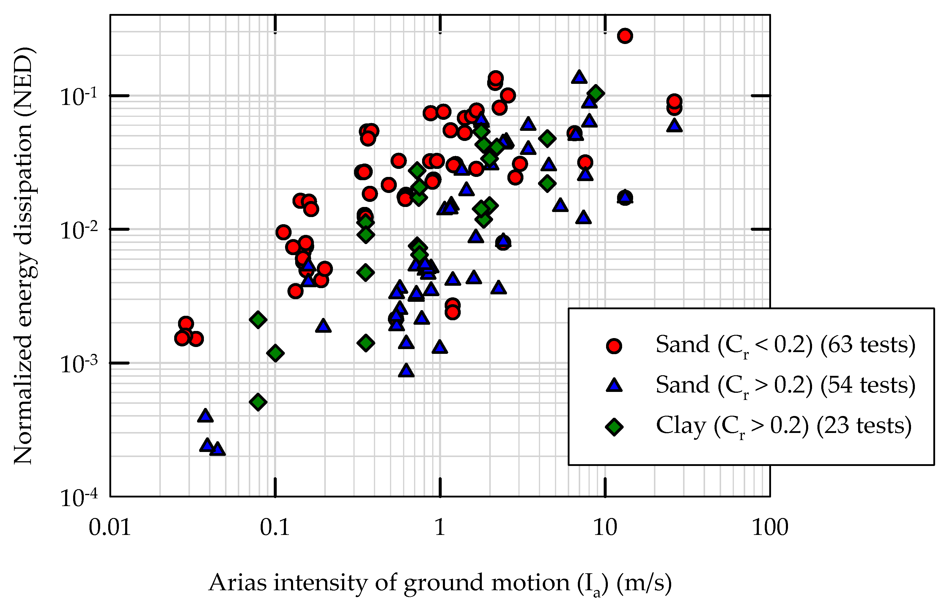
In machine learning, the representation of the problem using the best possible combination of input features, avoiding redundant features, and scaling and normalizing feature values is more important than using a more complicated machine learning algorithm [39]. For this study, A/Ac and amax are selected as two key input features, as the rocking moment capacity mainly depends on A/Ac (Equation (3)) and amax is the arguably the most commonly used seismic demand parameter in geotechnical earthquake engineering [66]. The slenderness ratio of the rocking system (h/B, which is also approximately equal to the applied normalized moment-to-shear ratio at the base of the footing during rocking) is chosen as another input feature as relatively taller (slender) rocking systems tend to rotate more than shorter rocking systems [65]. In addition, the rocking coefficient (Cr) of rocking system and Arias intensity of earthquake (Ia) are chosen as input features to model NED (this is supported by the apparent trends present in the experimental results shown in Figure 2). Cr incorporates the combined effects of footing dimensions, depth of embedment, shear strength and stiffness properties of soil, slenderness ratio of structure, and self-weight of the structure. As total seismic energy dissipation is cumulative, and depend on the amplitude, duration, frequency content, and number of cycles of loading, and the calculation of Ia does take those factors into account, Ia is chosen as one of the input features.

3.3. Performance Parameter: Normalized Energy Dissipation (NED)

It has been shown that the seismic energy dissipation in soil due to rocking reduces the maximum horizontal acceleration transmitted to the structure, e.g., [14,16,33]. The reduction in maximum horizontal acceleration at the effective center of gravity of the structure in turn reduces the base shear force and bending moment transmitted to the base of the column or shear wall of the structure. Since the base shear coefficient (Cy) is one of the key parameters used in seismic design of structures, seismic energy dissipation of rocking foundation is considered as the performance parameter (output parameter or prediction parameter of machine learning models) in this study. Total (cumulative) seismic energy dissipation in foundation soil (E) during rocking is calculated from the total area enclosed by the cyclic moment-rotation hysteretic loops of soil–foundation system. E is normalized by V and B in order to obtain a nondimensional parameter, called normalized energy dissipation (NED = E/(V·B)), and to make comparisons meaningful across different experiments and predictions (Equation (7)).
NED = 1 V · B · 0 θ fin M · d θ
In Equation (7), θfin is the last data point in foundation rotation time history at the end of the shake. It should be noted that the seismic energy dissipation through shear-sliding mode is not included in NED calculations. It has been shown that the energy dissipation through shear-sliding mode is negligible when compared to that of through moment-rotation mode for rocking dominated systems [65]. The normalized applied moment-to-shear ratio at the base of the footing are greater than 1.0 in the experiments (i.e., slenderness ratio of the rocking system, (h/B) > 1.0), and hence all the structure-foundation systems considered in this study are rocking dominated systems.
The data from the above mentioned database for 140 individual experiments have been processed to calculate NED and their corresponding input features [14,63]. Figure 2 presents the variation of NED due to foundation rocking with Arias intensity of earthquake ground motion (Ia) for different clusters of rocking coefficients (Cr) of rocking systems and separately for sandy and clayey soil foundations. As can be seen from Figure 2, NED appears to have some correlation with two of the chosen input features (Ia and Cr). However, the variation in the data in Figure 2 is so significant that simple, commonly used statistical models cannot be used to correlate NED with individual input features with reasonable accuracy. For example, when the data presented in Figure 2 for NED (all 140 instances) are run through a simple linear regression algorithm, with log (Ia) as independent variable and log (NED) as dependent variable, it results in a coefficient of determination (R2 value) of 0.22. This indicates that (i) the amount of variation in data is relatively high and (ii) simple linear regression model is not capable of correlating the data with reasonable accuracy. The experimental data presented in Figure 2 also shows that the foundation soil type could also be a possible variable to separate (or classify) NED values. Soil type has been considered as an input feature (as a binary variable) to machine learning algorithms; however the inclusion of soil type does not make significant difference in regression predictions (or in some cases, it makes the generalization weaker), and hence it is not considered as one of the input features in this study (to maintain the simplicity of models while not compromising the generalizability and accuracy).
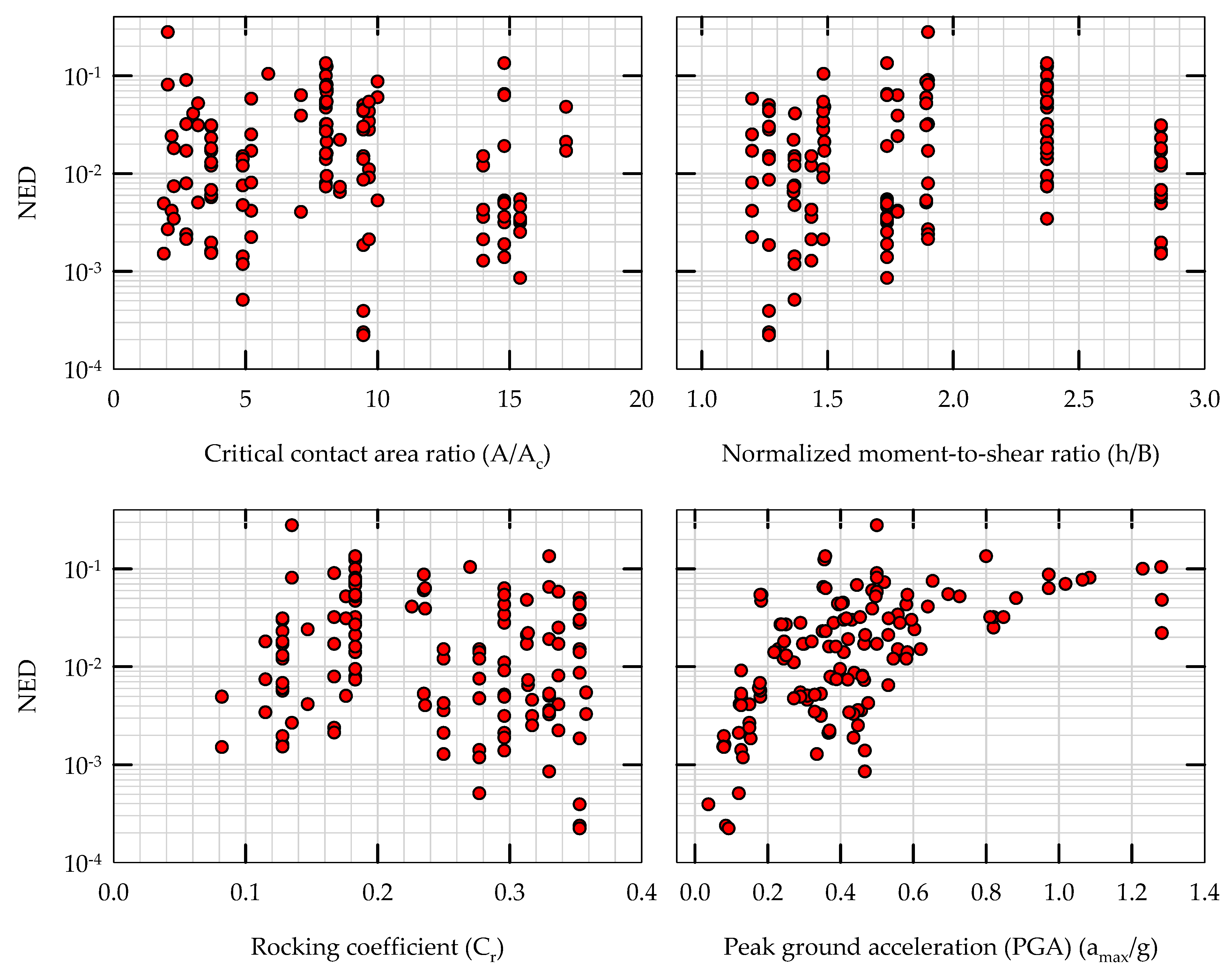
Figure 3 presents the experimental data (the same 140 experiments presented in Figure 2) for the variation of NED with the other four input features chosen in this study (A/Ac, h/B, Cr and amax/g) separately. As can be seen from Figure 3, the NED does not show any reasonable correlations with the input features, when plotted as a function of each of these input features separately (perhaps barring amax, which seems to show some correlation, though the variation is high). Once the moment reaches the ultimate moment of rocking foundation, any additional increase in amax does not increase the moment, and hence no further increase in NED. However, Ia, which includes the duration of ground motion (and hence indirectly the number of cycles of loading), on the other hand, correlates better with NED, as the cumulative NED depends on the number of cycles of loading. Overall, the experimental results presented in Figure 2 and Figure 3 show that NED cannot be correlated with any one of the input features alone with reasonable accuracy. Therefore machine learning algorithms, with multiple input features, are used in this study to discover the hidden relationships in data in multi-dimensional input feature space, to learn from the data, and to generalize the experimental patterns observed. That is, if the data points were plotted in higher dimensional space and if there were trends or relationships between multiple input features and NED, it would be hard to visualize these trends (i.e., making sense of the data in n-dimensional space would be difficult without using smart algorithms). As described in Section 4, the KNN and SVR algorithms, for example, analyze the data points in higher dimensional space either using distances between data points or using mapping functions (kernels) and hence are able to identify these relationships that are not apparent in two or three dimensional space.

3.4. Feature Transformation and Normalization

As can be seen from Figure 2, the variation (numerical range) in NED and Ia is relatively high, and hence the data is plotted in log–log space. For this reason, these two parameters (NED and Ia) are transformed to logarithmic values (base 10) before the training and testing phases of machine learning models. In addition, in order to make reliable predictions using models developed by different machine learning algorithms, all the input feature data are normalized so that each input feature value varies between 0.0 and 1.0. The following expression describes the input feature normalization process,
x i   i   [ x i x min x max x min ]
where x represents the input feature vector, xmin and xmax represent the minimum and maximum values of that input feature, respectively, and the subscript “i” goes from 1 to 5 (one vector each for each input feature).

4. Machine Learning Algorithms

Three nonlinear, nonparametric machine learning algorithms are considered in this study: distance-weighted k-nearest neighbors regression (KNN), support vector regression (SVR) and decision tree regression (DTR). k-nearest neighbors, support vector machines and decision trees are widely used and popular for classification problems in machine learning [37,38,39,40]. In this study, the modified versions of these algorithms, available in scikit-learn (also known as sklearn) library of modules in Python (https://scikit-learn.org/stable/, accessed on 1 September 2021), are used as regression models. Nonparametric machine learning algorithms do not make strong assumptions about the form of the mapping function between the input features and output variable and hence they are more flexible and free to learn any functional form from the training data. They tend to have complex, nonlinear decision boundaries or hyperplanes in multi-dimensional input space to predict the output variable. The fundamental principles of the three chosen regression algorithms and how they are used in supervised learning in this study are briefly described in the following sections.

4.1. Weighted k-Nearest Neighbors Regression (KNN)

Every machine learning algorithm has an inductive bias or a learning bias (i.e., the way its learning objectives are defined and how it makes predictions on future unseen data). The inductive bias of KNN algorithm is based on the assumption that when input data points are plotted (as vectors) in multi-dimensional input feature space, the data points that lie closer together share similar properties (i.e., similar output or prediction values). Therefore, if there are hidden relationships between multiple input features and the prediction variable, the KNN model is able to learn those relationships through training data. In this study, the Euclidean distance measure in n-dimensional space is used to calculate the distance between two data instances (n = 5 in this study; one for each input feature). In KNN, the entire training data is stored in the model during training phase. Essentially the KNN model does not require training in the traditional sense, however, the number of nearest neighbors (k) that determine the output is a hyperparameter in KNN model, which needs fine tuning. Relatively smaller values of k tend to overfit the training data, while relatively larger values of k tend to underfit the training data [39].
When a test data instance is fed as input, the KNN algorithm runs through the entire training dataset and finds k number of training instances that are closer to the test instance. The distance-weighted KNN regression model weighs the output values by the inverse of their distance from the test data point to its nearest neighbors and produces an output that is the weighted average of the output values of the nearest neighbors (i.e., closer neighbors of a test data point will have a greater influence on the output than neighbors that are further away). This results in a more complex nonlinear decision boundary of KNN model (for comparison, simple linear regression and multivariate linear regression algorithms use linear decision boundaries). The optimum value of k of KNN model is found to be 3 for the problem considered and k = 3 is used for all cases presented in this paper, except in hyperparameter tuning phase (Section 5.2).

4.2. Support Vector Regression (SVR)

It has been well documented that support vector machines (SVM) are well suited for classification of complex, nonlinear, small to medium sized datasets [38]. The objective of SVM algorithm is to find a hyperplane in an n-dimensional input space that distinctly separates the data points. The data points on either side of the hyperplane that are closest to the hyperplane are called support vectors. These data points influence the position and orientation of the hyperplane and help build the SVM. The margin (ϵ) is the distance from the hyperplane to the closest data point (support vector) in n-dimensional space. The support vectors are chosen in such a way that the hyperplane will be at a possible maximum distance from support vectors (by maximizing the margin). The major difference between SVM and SVR is that whereas SVM classification algorithm tries to fit the largest possible margin between different classes while limiting margin violations of data points (soft margin classifier), SVR algorithm tries to fit as many training data instances as possible within the margin while limiting margin violations of data points. The inductive bias of SVR is that it assumes that data points that have distinct characteristics tend to be separated by wide margins. In SVR, hyperplanes are decision boundaries that is used to predict the continuous output for performance parameter.
The major parameter of SVR algorithm is the kernel that is used to map (transform) the data instances (input data) into n-dimensional space. The radial basis function (RBF) kernel is used in this study as it is the most widely used kernel in SVR and it has the flexibility of dealing with nonlinear data [39,40]. Since complex, nonlinear data cannot be separated perfectly by a hyperplane, a wiggle room is allowed for the margin using additional set of parameters called slack variables in SVR. A hyperparameter called the cost parameter or penalty parameter (C) defines the magnitude of this wiggle room across all dimensions in input space (it is related to the penalty applied to the slack variables). As C affects the number of data instances that are allowed to fall within the margin, C influences the number of support vectors used by the model. Relatively larger values of C tend to overfit the training data, while relatively smaller values of C tend to underfit the training data. The optimum value of C of SVR model is found to be 1.0 for the problem considered and C = 1.0 is used for all cases presented in this paper, except in hyperparameter tuning phase (Section 5.2). Unlike other regression models (e.g., multivariate linear regression) that try to minimize the error between the actual and predicted value, the SVR tries to fit the best hyperplane within a threshold value (ϵ). This property makes the SVR to be less sensitive to outliers than the quadratic loss functions used in most regression models.

4.3. Decision Tree Regression (DTR)

Classification and regression trees (CART) are also nonlinear, non-parametric machine learning algorithms that use supervised learning technique to build a tree-like data structure. During the learning (training) phase, a decision tree breaks down a dataset into smaller and smaller subsets using binary rules, while at the same time associated decision trees (sub-trees) are incrementally developed. Typically, the core algorithm for building decision trees employs a top-down, greedy search through the space of possible branches using information gain as a measure of reduction in randomness in data (reduction in uncertainty or reduction in entropy in data). The DTR model used in this study maximizes the information gain by minimizing the mean absolute error while building the tree (i.e., when deciding a split, the decision is made based on the weighted average of the mean absolute errors of the two groups that create). The inductive bias of DTR model is based on the assumption that shorter trees are better than longer (deeper) trees and that the trees that place high information gain attributes close to the root of the tree are better than those that do not [38]. The major hyperparameter of the DTR is the maximum depth of the tree, as deeper trees tend to overfit the training data while relatively shorter (shallow) trees tend to underfit the training data. The optimum value of maximum depth of tree in DTR algorithm is found to be 6 for the problem considered in this study and maximum depth = 6 is used for all cases presented in this paper, except in hyperparameter tuning phase (Section 5.2).
During testing or prediction phase, the DTR model arrives at an estimate by asking a series of questions to the data related to input feature values, each question narrowing the possible values until the model gets confident enough to make a prediction. That is, given a test data point, the DTR model runs it through the entire tree asking a series of true or false questions until it reaches a leaf node. The final prediction is the average value of the dependent (prediction) variable in that leaf node. Other hyperparameters of DTR algorithm include minimum number of samples required to split an internal tree node, minimum number of samples required to be at a leaf node, and the maximum number of features to consider when looking for the best split. Note that all of these parameters are kept at their commonly used default values in the DTR algorithm available in the scikit-learn library in Python; only the maximum depth of the tree is varied in hyperparameter tuning phase of DTR model.

5. Results and Discussion

The initial evaluation of machine learning models using training and testing results (using a pair of randomly created training and testing datasets) are presented first and it is followed by the results of hyperparameter tuning of models, comparison of different model performances, and repeated k-fold cross validation tests of the models (5-fold and 7-fold cross validation tests with number of repeats = 3). The key evaluation metric used in this study is the mean absolute percentage error (MAPE) and it is defined by,
MAPE = 1 n · i = 1 n ( | i y i y i | )
where y is the actual output value, ỹ is the predicted output value, and the subscript “i” runs from 1 up to the number of predictions (n). MAPE is preferred and chosen over the commonly used root mean square (RMS) error measure in machine learning models, because MAPE is independent of the actual numerical values of the performance parameter (by normalization). In addition, for the purpose of comparisons, a multivariate linear regression (MLR) model is also developed using the same input features and supervised learning technique. As the MLR model is a linear, parametric model, it is used as the baseline model for comparison of model performances. Coefficient of determination (R2 value) is also used to compare the model performances wherever appropriate. It should be noted that no arbitrary threshold limit is set for MAPE value to classify whether the model predictions in terms of MAPE are acceptable or not for the chosen performance parameter (NED). In the following sections, comparisons are made using the MAPE values of all the machine learning models developed in this study and in the previous research on the same problem [58], wherever appropriate. Establishing a threshold value for MAPE of predicted NED would require a detailed study involving the consequences of energy dissipation of rocking foundations on the seismic response of structural systems they support in a performance-based engineering framework.

5.1. Initial Training and Testing of Models

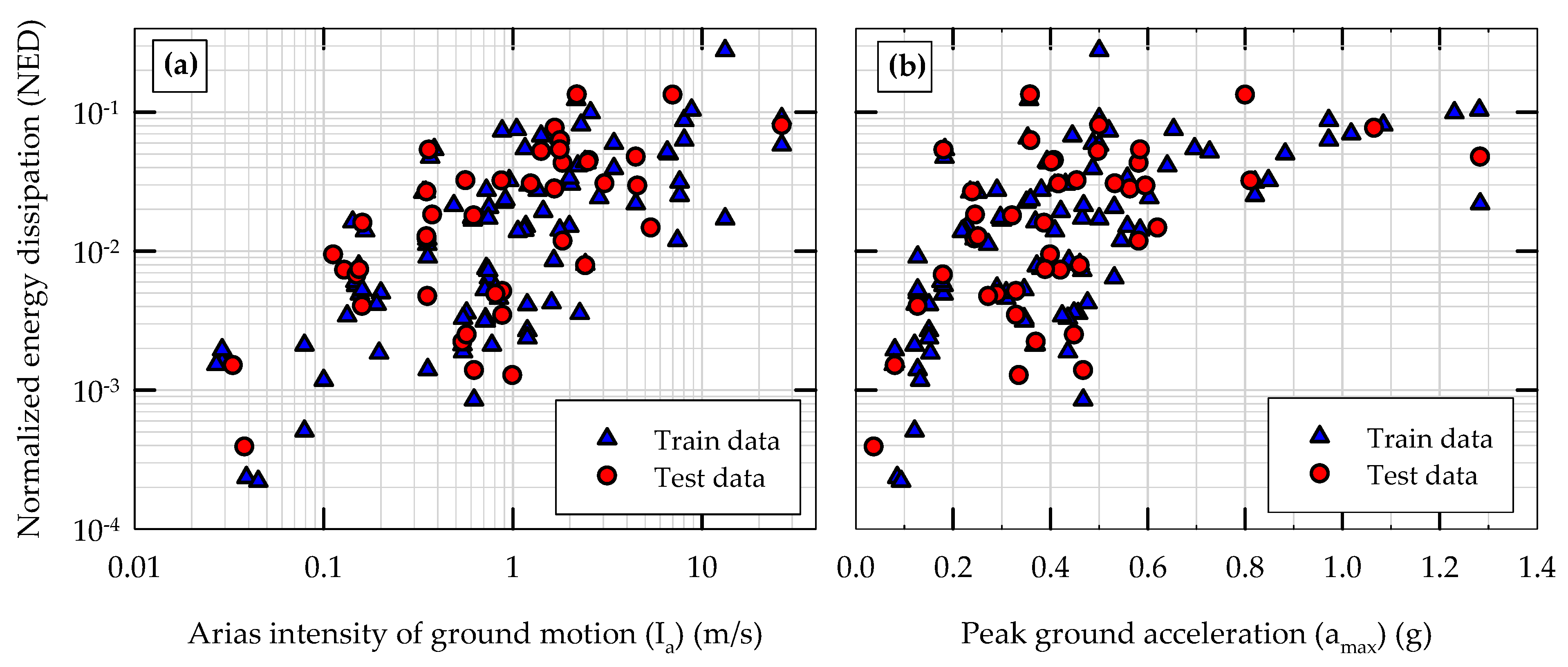
Altogether, 140 experimental data (instances) are extracted from the above-mentioned database and are split into two groups for the purpose of initial training (supervised learning) and testing of machine learning models. It should be noted that though the database currently has data obtained from 200 experiments, only 140 experiments are used in the current study, as other experiments involved either unsaturated sand or base shaking loading in an arbitrary direction. A 70–30% split is used to randomly create a training dataset (98 instances) and a testing dataset (42 instances) using the train-test-split function available in sklearn library of modules in Python. The 70–30% split is similar to the rule of thumb methods commonly used in supervised machine learning, e.g., [40]. Note that the random-state variable in this function is kept constant for this splitting of data for training and testing of all the models (i) to ensure consistency between different machine learning models and (ii) to ensure repeatability of results. It should be noted that this initial 70–30% split does not include a separate validation dataset, as repeated k-fold cross validations, considering the entire dataset (140 instances), are carried out separately (presented in Section 5.3). Figure 4 presents this split of data in NED versus Ia space and NED versus amax space. This train-test split is created randomly, and as a result, both training and testing sets of data cover wide range of values for input features and prediction variable reasonably well. The models are first trained using the training dataset, and in order to check the applicability of the models to represent the training data and to quantify what the models have learned from the training data, all three machine learning models are first tested using the same training dataset (i.e., how well the models predict the same data that are used to train the models). The models are then tested using the testing dataset.
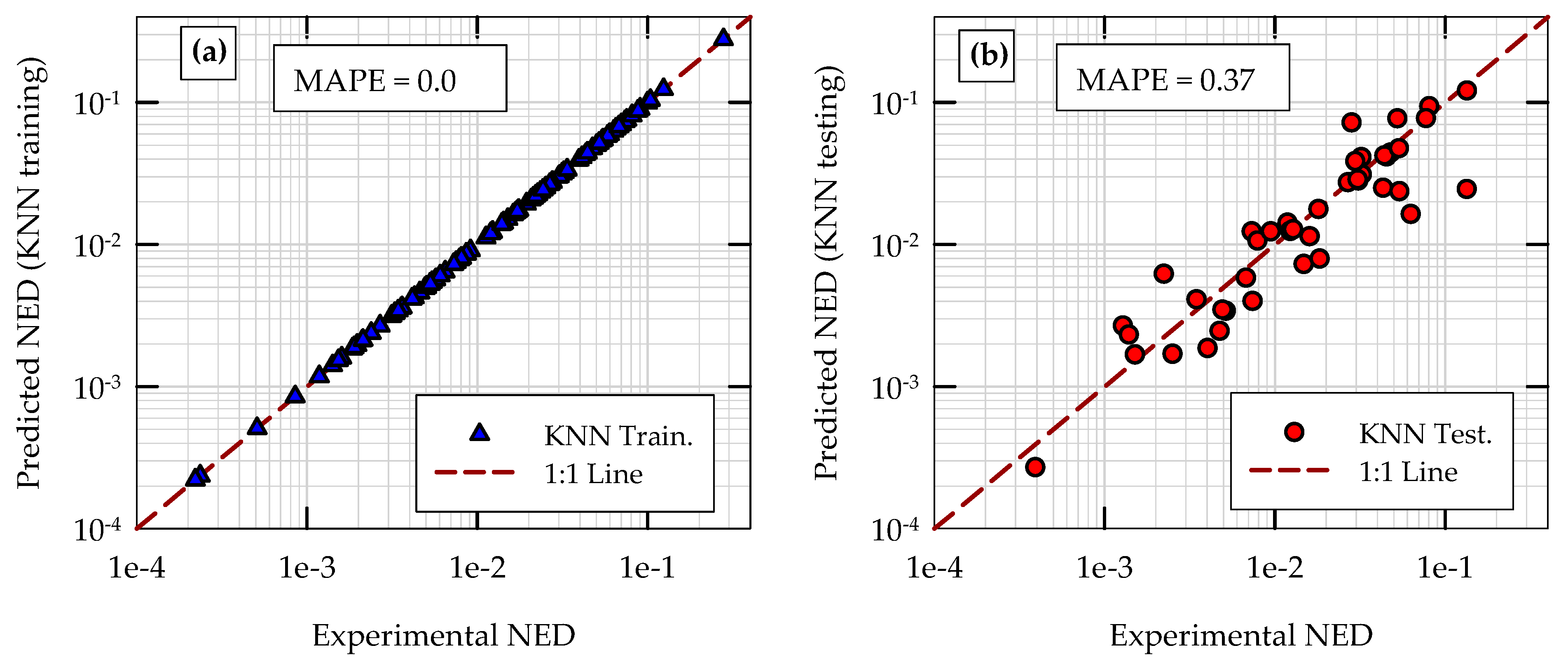
The variation of predicted NED with their corresponding experimental NED values on top of a 1:1 prediction-to-experiment comparison line are presented in Figure 5a,b for training phase and testing phase, respectively, of KNN model (with k = 3). As stated above, for KNN model, training phase simply means storing the entire training dataset in the model. As the distance-weighted KNN regression model weighs the output values by the inverse of their distance from the test data point to its nearest neighbors, when tested using the same training data points, the model captures the exact data point (because the distance is zero) and produces a perfect, flawless performance (MAPE = 0) (Figure 5a). This is expected of KNN model because of the weighing function used and this does not mean that the KNN model overfits the training data (discussed further in Section 5.2). During the testing phase of KNN model, the predictions are made by comparing every test data instance (previously unseen data) with already stored training data in the model using the weighing function described above. As can be seen from Figure 5b, the KNN model performs well during testing phase with a mean absolute percentage error (MAPE) of 0.37. The performance of KNN model also confirms that there exists a reasonable relationship between multiple input features as a vector in n-dimensional space and the prediction parameter.
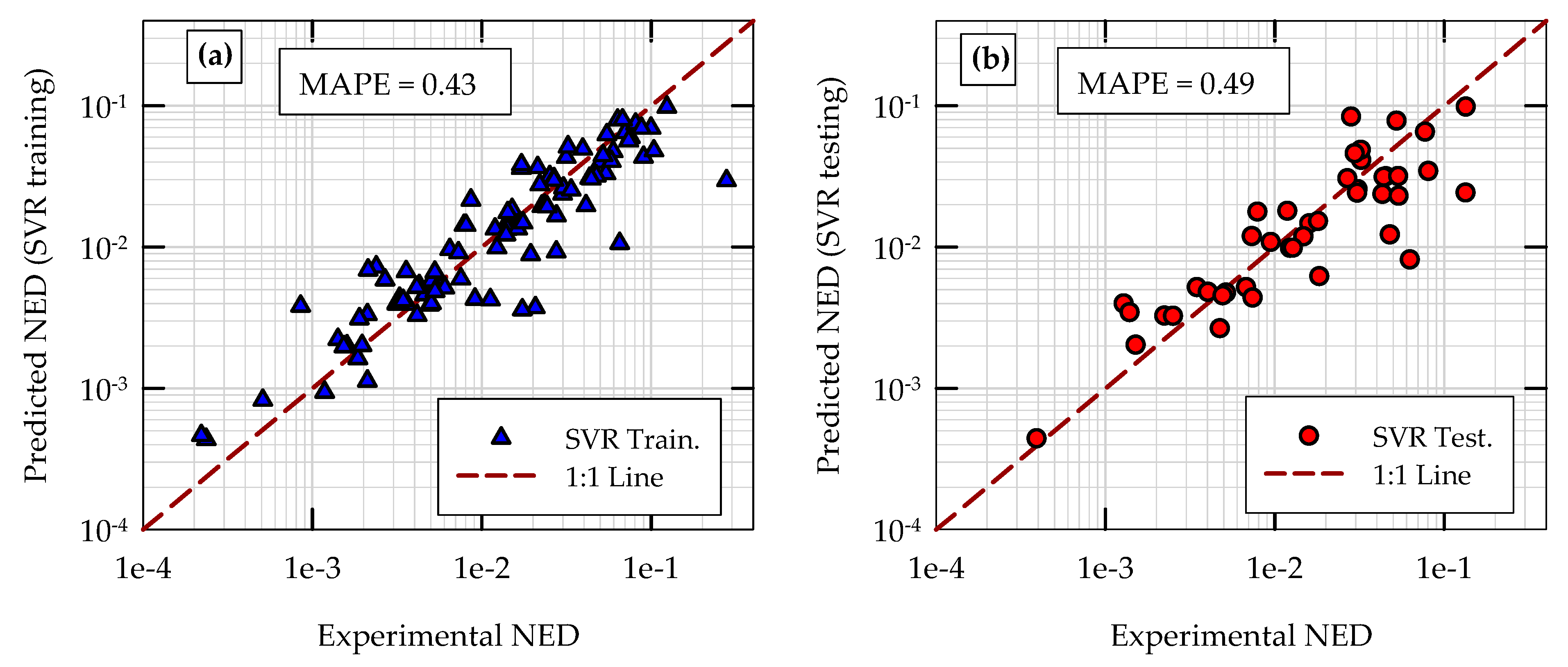
The variation of predicted NED with their corresponding experimental NED values on top of a 1:1 prediction-to-experiment comparison line are shown in Figure 6a,b for training phase and testing phase, respectively, of SVR model (with C = 1.0). For fair comparison, the same training and testing data sets (as in KNN model above) are used in SVR model as well. When the SVR model is tested with the same dataset that is used to train the model, it gives a MAPE of 0.43 (Figure 6a), and as can be seen from Figure 6b, when the SVR model is tested with previously unseen test data, the SVR model performs reasonably well with a MAPE of 0.49. Unlike the KNN model and DTR model (presented below), where the MAPE values on training and testing data are significantly different, for SVR model, the MAPE values on training and testing data are relatively close. This is consistent with the way how the SVR model works: while regression models, in general, try to minimize the error between the actual and predicted value, the SVR tries to fit the best hyperplane within a threshold value (epsilon). That is, the SVR model does use a strict loss function to minimize the error, and this results in more flexibility and more generalization of the model as can be seen from the model performance in testing phase (Figure 6b). The value of epsilon used for all the SVR models developed in this study is 0.1 (the default value recommended in scikit-learn library of modules in Python). It should be noted that the value of epsilon was varied and the results of SVM predictions were obtained for different values of epsilon. It was found that as long as epsilon is in between 0.01 and 1.0, the model predictions are not sensitive to the value of epsilon.
The variation of predicted NED with their corresponding experimental NED values on top of a 1:1 prediction-to-experiment comparison line are shown in Figure 7a,b for training phase and testing phase, respectively, of DTR model (with maximum depth of tree = 6). As in the case for KNN and SVR models, the DTR model is first tested using the same data points that are used to train the model and build the tree (98 data instances), and the predicted results are presented in Figure 7a. From the predicted versus experimental NED comparisons and with a MAPE of 0.21, it can be said that the DTR model learns well enough to build a reasonably good tree structure during the training phase. The “horizontal trends” the data points show in Figure 7a are compatible with how the DTR regression model works: it uses the average value of the prediction variable when the tree reaches a leaf node. DTR model predictions during testing phase (for 42 previously unseen data instances) are shown in Figure 7b. The MAPE on test data is higher for DTR model (0.83), when compared to KNN and SVR models. However, as will be seen later, the DTR model is still better than MLR model in terms of average MAPE in k-fold cross validation tests (discussed in Section 5.4).

5.2. Hyperparameter Tuning of Models

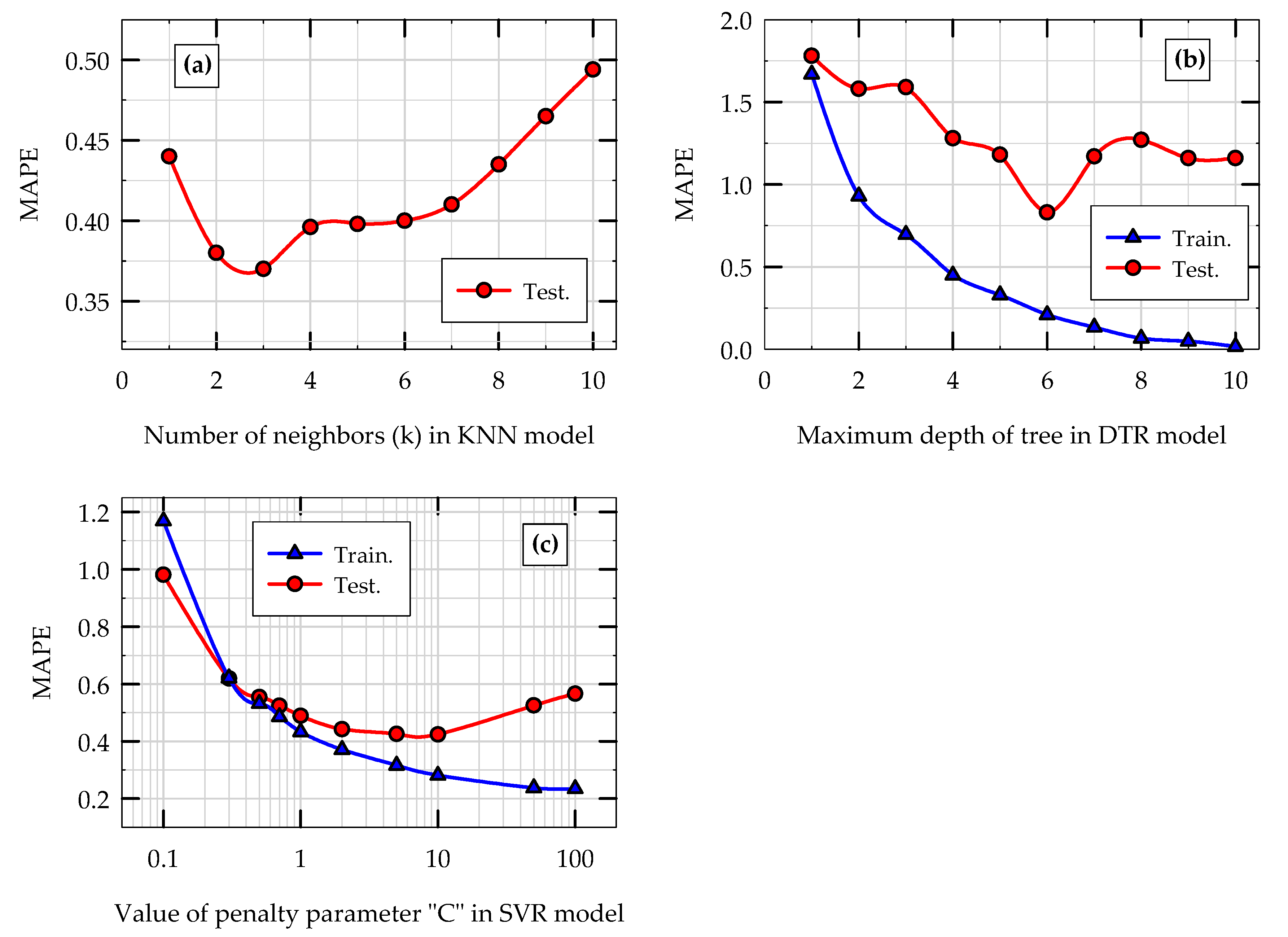
For the three machine learning models presented above, hyperparameter tuning is carried out (i) to investigate the sensitivity of model predictions to their hyperparameters, (ii) to determine the optimum values of these parameters for the problem considered and data analyzed, and (iii) to ensure that the models neither overfit nor underfit the training data. The number of nearest neighbors (k), the maximum depth of the tree, and the cost or penalty parameter (C) are varied for KNN, DTR and SVR models, respectively, and the corresponding MAPE values of predictions are calculated. The results are presented for training phase and testing phase of all three models separately in Figure 8.
For the KNN model, the variation of MAPE with k during training phase of the model (i.e., when the same training data is used to test the model) is not shown in Figure 8a because the KNN model predicts the exact (experimental) value for NED for all values of k during training phase. This is because of the nature of the weighing function used: it is inversely proportional to the distance from the test point to the closest neighbors and it varies from infinity to zero as the distance varies from zero to infinity. This results in MAPE = 0 regardless of the k value in training phase because the weight of the exact match is infinity and hence that match dominates over other neighboring data points. If a slightly different weighing function were used, the MAPE would increase with the number of neighbors considered when tested with the training data. For example, in a previous study on the same topic, a different weighing function was used in KNN model: the weight varies from 1.0 to 0.0 as the distance varies from 0.0 to infinity [58]. For the aforementioned weighing function, when k = 1 during training phase, the model would give zero error by overfitting the training data, however, as the value of k increases, the MAPE would increase. The MAPE during testing phase of KNN model, on the other hand, first decreases as k increases and then increases as k increases further (Figure 8a). This is also a typical behavior of the KNN algorithm when tested with previously unseen test data [39,58]. The minimum MAPE during testing was obtained when k is equal to 3, and based on this observation, k = 3 is taken as the “sweet spot” of the KNN algorithm for the problem considered, and all other results of KNN model presented in this paper are obtained using k = 3. This value of k is also consistent with the results presented in [58]. Any value smaller than 3 for k would overfit the training data and any value greater than 3 for k would underfit the training data.
For DTR model (Figure 8b), MAPE values during training phase decreases as the maximum depth of tree increases, as expected. For shallow tress, the model underfits the training data (high MAPE values), and as the maximum depth of the tree increases (deep trees), the DTR model is free to grow as big a tree as possible to try to match as many training data instances as possible (overfitting the training data and hence results in small MAPE values on training data). Neither a very shallow tree nor a very deep tree is preferred and an optimum value for maximum depth of the tree is needed. The MAPE values during testing phase of DTR model, on the other hand, first decreases and then increases as the maximum depth of tree increases, with the optimum maximum depth of the tree being 6. Any value smaller than 6 for maximum depth of tree would underfit the training data and any value greater than 6 for maximum depth of tree would overfit the training data. Based on this observation, maximum depth of tree for optimum performance of DTR model is found to be 6 for the problem considered, and all other results of DTR model presented in this paper are obtained using maximum depth of tree = 6.
Similar to the trend observed for DTR model, for SVR model (Figure 8c), The MAPE values during training phase decreases as the value of penalty parameter C increases, as expected. Larger values of C means bigger penalty and hence results in relatively smaller number of data points that violate the margin (poor generalization). Neither a very small value for C (underfitting the training data) nor a very high value for C (overfitting the training data) is preferred. The MAPE values during testing phase of SVR model, on the other hand, first decreases and then increases as C increases, with the optimum value of C being between 5 and 10. However, based on the results obtained in multiple, repeated k-fold cross validation of SVR model (presented in Section 5.4), C = 1.0 is found to be the best choice for the optimum value of C for problem considered. All other results of SVR model presented in this paper are obtained using C = 1.0.

5.3. Comparison of Model Performances in Initial Training and Testing Phases

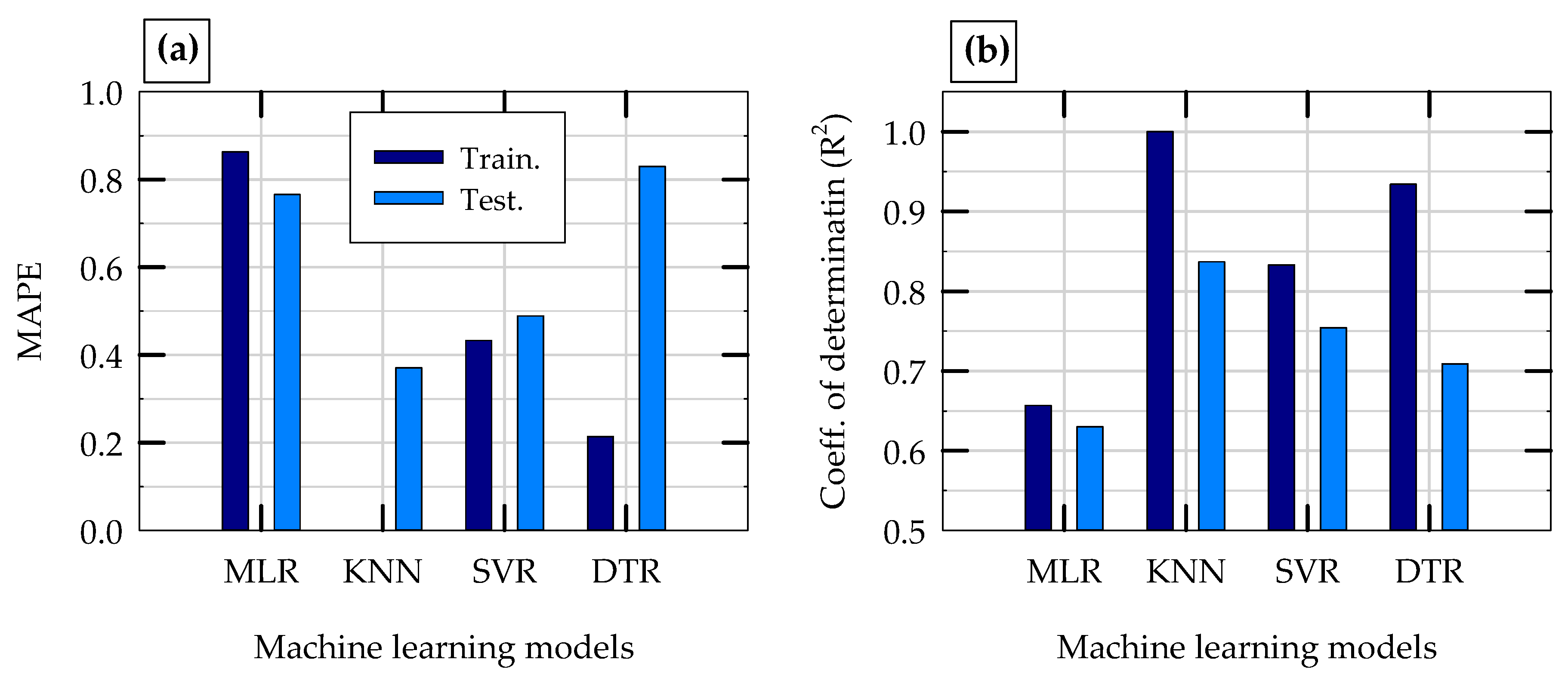
Figure 9a presents an all-error comparison for different scenarios to compare and contrast the performance of different machine learning models based on the MAPE values in the prediction of NED in initial training and testing phases of the models. Also included in the figure are the MAPE values of multivariate linear regression model (MLR) developed using the same input features and the same training and testing datasets. MLR is a linear, parametric model, where a hyperplane is used to model the relationship between the output and multiple input variables as expressed by Equation (10).
log ( NED ) = β 0 + β 1 · ( A A c ) + β 2 · ( h B ) + β 3 · C r + β 4 · a max + β 5 · log ( I a )
The best combination of coefficients (β values) are calculated using training data by minimizing the sum of square of errors. The MLR model is used here as a baseline model for comparison. Figure 9b plots the coefficient of determination (R2) values between the experimental and predicted values of NED of all models during initial training and testing phases. It should be noted that the smaller the MAPE values the better the performance of the model and the greater the R2 values the better the predictions of the model when compared to experimental data.
Based on the MAPE values and R2 values of the models on training and testing data, it is apparent that all three nonparametric machine learning models developed in this study (KNN, SVR and DTR) perform better than the MLR model. The only exception is the MAPE value of the DTR model on test data (0.83), which is slightly higher than that of the corresponding MAPE value of MLR model (0.77). Interestingly, the MAPE of the DTR model on training data is the second smallest (0.21) of all four models during training phase (second only to KNN model, which has a training MAPE of 0.0 and a corresponding R2 value of 1.0 for reasons discussed in Section 5.2). Among the three nonparametric models, both KNN and SVR models outperform the DTR model, and between KNN and SVR models, it appears that the KNN model performance is better than SVR model. However, it is worth mentioning that of all the models, the SVR model is the most consistent in terms of MAPE and R2 values during training and testing phases (more on this is presented in Section 5.4). For all three nonparametric models, the testing MAPE values are greater than those in training phase while the testing R2 values are smaller than those in training phase. This trend is a typical characteristic of machine learning models, especially when the size of the data is relatively small. The repeated k-fold cross validation test results (based on complete random shuffling and multiple splitting of data) are presented below to complement this error comparison and to make better comparisons between models by eliminating the effect of a single split of training and testing datasets on the performance of models.

5.4. Repeated k-Fold Cross Validation Tests of Models

A machine learning model with relatively lower bias performs better in terms of accuracy on complicated problems, whereas a machine learning model with relatively lower variance is less sensitive to changes in training data [34]. Both lower bias and lower variance are preferred, however, it is difficult to achieve both in a single machine learning model in general (commonly referred to as the bias-variance trade-off). The k-fold cross validation is a technique for evaluating the performance of machine learning models on multiple, different train-test splits of dataset. It provides a measure of how good the model performance is both in terms of accuracy and variance. A single run of k-fold cross validation may result in noisy results for model error (MAPE) and hence multiple runs are carried out by varying k (number of folds) and by using random sampling each time. In this study, the complete dataset is randomly shuffled and split into different groups of train-test sets for k = 5 and 7. On top of this, for each of 5-fold and 7-fold cross validations, the process is repeated three times (number of repeats = 3) with different randomization of the data in each repetition (repeated k-fold cross validation). With this setup, for each model, the repeated 5-fold and 7-fold cross validation tests result in 15 and 21 values, respectively, for testing MAPE.
Figure 10 presents the results of (a) repeated 5-fold cross validation test and (b) repeated 7-fold cross validation test for all four machine learning models considered in this study. In each case, results obtained for testing MAPE are plotted in the form of boxplots. For each machine learning model, the boxplot plots the average of MAPE (triangles), median of MAPE (the horizontal line inside the box), 25th and 75th percentile values of MAPE (bottom and top edges of the box), 10th and 90th percentile values of MAPE (bottom and top horizontal lines outside the box), and the extreme values of MAPE (5th and 95th percentiles, represented by circles). Comparing Figure 10a with Figure 10b, it is clearly seen that the average values of MAPE in repeated 5-fold and 7-fold cross validation tests are very close to each other for all four models (0.46 and 0.44 for KNN, 0.54 and 0.52 for SVR, 0.80 and 0.78 for DTR, and 0.89 and 0.90 for MLR), highlighting the overall consistency of all four models (i.e., statistically speaking, the results presented herein are not produced by random chance). The average MAPE values of the models alone suggest that, for the problem considered, the overall accuracy of model predictions follows the following order, from the most accurate to the least accurate: KNN, SVR, DTR, and MLR. However, SVR model is the most consistent in terms of the variance in MAPE values in repeated k-fold cross validations. The total variance in MAPE (the difference between the two extreme values of MAPE) of SVR model is 0.43 and 0.57 in repeated 5-fold and 7-fold cross validations, respectively. The second most consistent model in terms of variance in MAPE is KNN, for which, the corresponding total variance in MAPE values are 0.62 and 0.69. The DTR model has higher variance when compared to other three models, however the accuracy (average MAPE) of DTR (around 0.8) is still better than that of the MLR model (around 0.9). It should be noted that, as discussed below, both the accuracy and variance of DTR model could be improved by using ensemble methods that combine multiple decision trees together such as bootstrap aggregation and boosting [38,39].

6. Discussion and Implications

The overall performance of KNN and MLR models developed in this study are an improvement to the previously published results on the same topic, when the same experimental data with slightly different input features were used [58]. The average MAPE values of KNN and MLR models developed in this study on the prediction of NED (in repeated k-fold cross validation tests) are around 0.45 and 0.9, respectively, while the corresponding values in the previous study are around 0.75 and 1.0, respectively [58]. This improvement can be attributed to (i) the additional input feature used in this study (slenderness ratio of the rocking system or applied moment-to-shear ratio on the foundation), (ii) the slightly different distance-weighing function used in the KNN algorithm, and (iii) the different input feature normalization function used in this study.
The performance of machine learning models developed in this study could be further improved by using ensemble methods. For example, stacked generalization (stacking) can be used to combine the machine learning models developed in this study to create an ensemble machine learning model using different combinations of base machine learning models. Similarly, bootstrap aggregation (bagging) and adaptive boosting (ada-boosting), for example, can be used to combine multiple DTR models to create ensemble models that would improve the accuracy and reduce the variance in predictions. The simple idea behind ensemble machine learning methods is that “groups of people can often make better decisions than individuals, especially when group members each come in with their own biases” [39]. Ensemble methods work best when (i) the individual models are as independent from one another as possible or (ii) the same base algorithm is trained on different subsets of the training dataset [38]. The three nonparametric base machine learning algorithms considered in this study (KNN, SVR and DTR) have different inductive biases, and hence combining them using ensemble methods is expected to produce better predictions in terms of accuracy and variance.
The machine learning models developed in this study could be combined with mechanics-based models used to simulate the rocking behavior of shallow foundations. Science-guided machine learning (also called theory-guided data science), a recently emerged paradigm, has been shown to successfully combine the beneficial features of both physics-based models and machine learning models while minimizing their adverse effects, e.g., [67,68,69,70]. The idea is to combine the mechanics that govern the physics of the rocking foundation problem with the knowledge learned from the use of big data and machine learning techniques to develop a hybrid mechanics-guided machine learning predictive framework that would ensure better generalizability and accuracy of predictions as well as scientific consistency of results. By combining mechanics based models with machine learning models, scientific knowledge would be used to guide the learning of machine learning algorithms, which can capture the hidden complicated relationships among the many rocking system parameters that are not captured by mechanics-based models.

7. Summary and Conclusions

7.1. Summary

Three nonlinear, nonparametric machine learning algorithms (KNN, SVR and DTR) are used to develop data-driven, predictive models for seismic energy dissipation of rocking foundations during seismic loading using supervised learning technique. Data mined from a rocking foundations database for critical contact area ratio, slenderness ratio (moment-to-shear ratio) and rocking coefficient of rocking system, and peak ground acceleration and Arias intensity of earthquake ground motion are used as input features to machine learning models. In addition to initial evaluation and analysis of the models using 70–30% train-test split of data instances, hyperparameter tuning of models, performance comparison of the models using MAPE and R2 values, and repeated 5-fold and 7-fold cross validation tests of the models using random sampling are also carried out.

7.2. Conclusions

Based on the results obtained in this study, the following conclusions are derived.
  • All three nonparametric machine learning models developed in this study (KNN, SVR and DTR) perform better than the parametric MLR model in capturing the complex relationship between NED and input features of rocking foundations.
  • The overall performance of KNN and MLR models developed in this study are an improvement to the previously published results on the same topic, when the same experimental data with slightly different input features were used [58].
  • Based on hyperparameter tuning of KNN, SVR and DTR models, k = 3, C = 1.0, and maximum depth of tree = 6, respectively, are found to be the optimum values for the respective hyperparameters for the problem considered.
  • Among all four machine learning models developed in this study, KNN model consistently outperforms all other models in terms of accuracy of predictions. The average MAPE of KNN model in repeated 5-fold and 7-fold cross validations are 0.46 and 0.44, respectively. The second most accurate model is SVR, for which the corresponding average MAPE values are 0.54 and 0.52. On average, the accuracy of KNN model is about 16% higher than that of SVR model.
  • Among all four machine learning models developed, SVR model is the most consistent in terms of training and testing errors as well as in terms of the variance in MAPE values in repeated k-fold cross validation tests. The total variance in MAPE of SVR model is 0.43 and 0.57 in repeated 5-fold and 7-fold cross validations, respectively. The second most consistent model in terms of total variance in MAPE is KNN, for which, the corresponding total variance in MAPE values are 0.62 and 0.69. On average, the variance of SVR model is about 27% smaller than that of KNN model.
  • The DTR model has higher variance when compared to all other three models, however, the mean accuracy of DTR model is still better than that of the MLR model. The overall average MAPE values of DTR is 0.79, which is still better than the corresponding MAPE value of MLR model (0.90). The accuracy and variance of DTR model could be improved by combining multiple DTR models together using ensemble methods such as bagging and boosting.
  • The data-driven predictive models developed in this study can be used in combination with other physics-based or mechanics-based models to complement each other in modeling of rocking behavior of shallow foundations in practical applications. One such recently emerged approach is theory-guided machine learning, where scientific knowledge is used as instructional guide to machine learning algorithms [67,68,69,70].

Funding

This research received no external funding.

Institutional Review Board Statement

Not applicable.

Informed Consent Statement

Not applicable.

Conflicts of Interest

The author declares no conflict of interest.

References

  1. Gajan, S.; Phalen, J.D.; Kutter, B.L.; Hutchinson, T.C.; Martin, G. Centrifuge modeling of load-deformation behavior of rocking shallow foundations. Soil Dyn. Earthq. Eng. 2005, 25, 773–783. [Google Scholar] [CrossRef]
  2. Gajan, S.; Kutter, B.L. Capacity, settlement, and energy dissipation of shallow footings subjected to rocking. J. Geotech. Geoenviron. Eng. 2008, 134, 1129–1141. [Google Scholar] [CrossRef] [Green Version]
  3. Shirato, M.; Kouno, T.; Asai, R.; Nakatani, S.; Fukui, J.; Paolucci, R. Large-scale experiments on nonlinear behavior of shallow foundations subjected to strong earthquakes. Soils Found. 2008, 48, 673–692. [Google Scholar] [CrossRef] [Green Version]
  4. Deng, L.; Kutter, B.L.; Kunnath, S.K. Centrifuge modeling of bridge systems designed for rocking foundations. J. Geotech. Geoenviron. Eng. 2012, 138, 335–344. [Google Scholar] [CrossRef]
  5. Drosos, V.; Georgarakos, T.; Loli, M.; Anastasopoulos, I.; Zarzouras, O.; Gazetas, G. Soil-foundation-structure interaction with mobilization of bearing capacity: Experimental study on sand. J. Geotech. Geoenviron. Eng. 2012, 138, 1369–1386. [Google Scholar] [CrossRef] [Green Version]
  6. Gelagoti, F.; Kourkoulis, R.; Anastasopoulos, I.; Gazetas, G. Rocking isolation of low-rise frame structures founded on isolated footings. Earthq. Eng. Struct. Dyn. 2012, 41, 1177–1197. [Google Scholar] [CrossRef]
  7. Anastasopoulos, I.; Loli, M.; Georgarakos, T.; Drosos, V. Shaking table testing of rocking—Isolated bridge pier on sand. J. Earthq. Eng. 2013, 17, 1–32. [Google Scholar] [CrossRef]
  8. Antonellis, G.; Gavras, A.G.; Panagiotou, M.; Kutter, B.L.; Guerrini, G.; Sander, A.; Fox, P.J. Shake table test of large-scale bridge columns supported on rocking shallow foundations. J. Geotech. Geoenviron. Eng. 2015, 141, 04015009. [Google Scholar] [CrossRef]
  9. Liu, W.; Hutchinson, T.; Gavras, A.; Kutter, B.L.; Hakhamaneshi, M. Seismic behavior of frame-wall-rocking foundation systems. II: Dynamic testing phase. J. Geotech. Geoenviron. Eng. 2015, 141, 04015060. [Google Scholar] [CrossRef]
  10. Ko, K.-W.; Ha, J.-G.; Park, H.-J.; Kim, D.-S. Centrifuge modeling of improved design for rocking foundation using short piles. J. Geotech. Geoenviron. Eng. 2019, 145, 04019031. [Google Scholar] [CrossRef]
  11. Sharma, K.; Deng, L. Characterization of rocking shallow foundations on cohesive soil using field snap-back tests. J. Geotech. Geoenviron. Eng. 2019, 145, 04019058. [Google Scholar] [CrossRef]
  12. Gavras, A.G.; Kutter, B.L.; Hakhamaneshi, M.; Gajan, S.; Tsatsis, A.; Sharma, K.; Kouno, T.; Deng, L.; Anastasopoulos, I.; Gazetas, G. Database of rocking shallow foundation performance: Dynamic shaking. Earthq. Spectra 2020, 36, 960–982. [Google Scholar] [CrossRef]
  13. Hakhamaneshi, M.; Kutter, B.L.; Gavras, A.G.; Gajan, S.; Tsatsis, A.; Liu, W.; Sharma, K.; Pianese, G.; Kouno, T.; Deng, L.; et al. Database of rocking shallow foundation performance: Slow-cyclic and monotonic loading. Earthq. Spectra 2020, 36, 1585–1606. [Google Scholar] [CrossRef]
  14. Gajan, S.; Soundararajan, S.; Yang, M.; Akchurin, D. Effects of rocking coefficient and critical contact area ratio on the performance of rocking foundations from centrifuge and shake table experimental results. Soil Dyn. Earthq. Eng. 2021, 141, 106502. [Google Scholar] [CrossRef]
  15. Kelly, T.E. Tentative seismic design guidelines for rocking structures. Bull. N. Z. Soc. Earthq. Eng. 2009, 42, 239–274. [Google Scholar] [CrossRef]
  16. Anastasopoulos, I.; Gazetas, G.; Loli, M.; Apostolou, M.; Gerolymos, N. Soil failure can be used for seismic protection of structures. Bull. Earthq. Eng. 2010, 8, 309–326. [Google Scholar] [CrossRef]
  17. Liu, W.; Hutchinson, T.C.; Kutter, B.L.; Hakhamaneshi, M.; Aschheim, M.A.; Kunnath, S.K. Demonstration of compatible yielding between soil-foundation and superstructure components. J. Struct. Eng. 2013, 139, 1408–1420. [Google Scholar] [CrossRef]
  18. Pecker, A.; Paolucci, R.; Chatzigogos, C.; Correia, A.A.; Figini, R. The role of non-linear dynamic soil-foundation interaction on the seismic response of structures. Bull. Earthq. Eng. 2014, 12, 1157–1176. [Google Scholar] [CrossRef]
  19. Kutter, B.L.; Moore, M.; Hakhamaneshi, M.; Champion, C. Rationale for shallow foundation rocking provisions in ASCE 41-13. Earthq. Spectra 2019, 32, 1097–1119. [Google Scholar] [CrossRef]
  20. American Society of Civil Engineers (ASCE). Seismic Evaluation and Retrofit of Existing Buildings; ASCE/SEI Standard 41-13; American Society of Civil Engineers: Reston, VA, USA, 2014. [Google Scholar] [CrossRef]
  21. Ntritsos, N.; Anastasopoulos, I.; Gazetas, G. Static and cyclic undrained response of square embedded foundations. Geotechnique 2015, 65, 805–823. [Google Scholar] [CrossRef]
  22. Kourkoulis, R.; Gelagoti, F.; Anastasopoulos, I. Rocking isolation of frames on isolated footings: Design insights and limitations. J. Earthq. Eng. 2012, 16, 374–400. [Google Scholar] [CrossRef]
  23. Gajan, S.; Raychowdhury, P.; Hutchinson, T.C.; Kutter, B.L.; Stewart, J.P. Application and validation of practical tools for nonlinear soil-foundation interaction analysis. Earthq. Spectra 2010, 26, 119–129. [Google Scholar] [CrossRef]
  24. Gajan, S.; Kayser, M. Quantification of the influences of subsurface uncertainties on the performance of rocking foundation during seismic loading. Soil Dyn. Earthq. Eng. 2019, 116, 1–14. [Google Scholar] [CrossRef]
  25. Allotey, N.; Naggar, M.H. Analytical moment-rotation curves for rigid foundations based on a Winkler model. Soil Dyn. Earthq. Eng. 2003, 23, 367–381. [Google Scholar] [CrossRef]
  26. Paolucci, R.; Shirato, M.; Yilmaz, M.T. Seismic behavior of shallow foundations: Shaking table experiments versus numerical modeling. Earthq. Eng. Struct. Dyn. 2008, 37, 577–595. [Google Scholar] [CrossRef]
  27. Raychowdhury, P.; Hutchinson, T.C. Performance evaluation of a nonlinear Winkler-based shallow foundation model using centrifuge test results. Earthq. Eng. Struct. Dyn. 2009, 38, 679–698. [Google Scholar] [CrossRef]
  28. Pelekis, I.; McKenna, F.; Madabhushi, S.P.G.; DeJong, M. Finite element modeling of buildings with structural and foundation rocking on dry sand. Earthq. Eng. Struct. Dyn. 2021, 50, 3093–3115. [Google Scholar] [CrossRef]
  29. Cremer, C.; Pecker, A.; Davenne, L. Cyclic macro-element of soil structure interaction: Material and geometrical nonlinearities. Int. J. Numer. Anal. Methods Geomech. 2001, 25, 1257–1284. [Google Scholar] [CrossRef]
  30. Gajan, S.; Kutter, B.L. Contact interface model for shallow foundations subjected to combined cyclic loading. J. Geotech. Geoenviron. Eng. 2009, 135, 407–419. [Google Scholar] [CrossRef]
  31. Chatzigogos, C.T.; Pecker, A.; Salencon, L. Macro element modeling of shallow foundations. Soil Dyn. Earthq. Eng. 2009, 29, 765–781. [Google Scholar] [CrossRef] [Green Version]
  32. Chatzigogos, C.T.; Figini, R.; Pecker, A.; Salencon, L. A macro element formulation for shallow foundations on cohesive and frictional soils. Int. J. Numer. Anal. Methods Geomech. 2011, 35, 902–931. [Google Scholar] [CrossRef]
  33. Gajan, S.; Godagama, B. Seismic performance of bridge-deck-pier-type-structures with yielding columns supported by rocking foundations. J. Earthq. Eng. 2019, 1–34. [Google Scholar] [CrossRef]
  34. Cavalieri, F.; Correia, A.A.; Crowley, H.; Pinho, R. Dynamic soil–structure interaction models for fragility characterization of buildings with shallow foundations. Soil Dyn. Earthq. Eng. 2020, 132, 106004. [Google Scholar] [CrossRef]
  35. OpenSees. Open System for Earthquake Engineering Simulations. Version 3.3.0.; Pacific Earthquake Engineering Research Center: Berkeley, CA, USA; University of California: Berkeley, CA, USA, 2021; Available online: https://opensees.berkeley.edu/ (accessed on 1 September 2021).
  36. Forcellini, D. Seismic Assessment of a benchmark based isolated ordinary building with soil structure interaction. Bull. Earthq. Eng. 2018, 16, 2021–2042. [Google Scholar] [CrossRef]
  37. Deitel, P.; Deitel, H. Introduction to Python for Computer Science and Data Science, 1st ed.; Pearson Publishing: New York, NY, USA, 2020. [Google Scholar]
  38. Geron, A. Hands-On Machine Learning with Scikit-Learn, Keras, and TensorFlow: Concepts, Tools and Techniques to Build Intelligent Systems, 2nd ed.; O’Reilly Media, Inc.: Sebastopol, CA, USA, 2019. [Google Scholar]
  39. Daume, H., III. A Course in Machine Learning. Version 0.99; Self-Published: College Park, MD, USA, 2013; Available online: http://ciml.info (accessed on 1 September 2021).
  40. Brownlee, J. Machine Learning Algorithms from Scratch with Python. Machine Learning Mastery. Version v1.9. 2019. Available online: https://machinelearningmastery.com/ (accessed on 1 September 2021).
  41. Ebid, A.M. 35 years of (AI) in geotechnical engineering: State of the art. Geotech. Geol. Eng. 2021, 39, 637–690. [Google Scholar] [CrossRef]
  42. Jeremiah, J.J.; Abbey, S.J.; Booth, C.A.; Kashyap, A. Results of application of artificial neural networks in predicting geo-mechanical properties of stabilized clays—A review. Geotechnics 2021, 1, 144–171. [Google Scholar] [CrossRef]
  43. Yang, Y.; Rosenbaum, M.S. The artificial neural network as a tool for assessing geotechnical properties. Geotech. Geol. Eng. 2002, 20, 149–168. [Google Scholar] [CrossRef]
  44. Das, S.K.; Samui, P.; Khan, S.Z.; Sivakugan, N. Machine learning techniques applied to prediction of residual strength of clay. Cent. Eur. J. Geosci. 2011, 3, 449–461. [Google Scholar] [CrossRef]
  45. Mozumder, R.A.; Laskar, A.I. Prediction of unconfined compressive strength of geopolymer-stabilized clayey soils using artificial neural network. Comput. Geotech. 2015, 69, 291–300. [Google Scholar] [CrossRef]
  46. Ayeldeen, M.; Yuki, H.; Masaki, K.; Abdelazim, N. Unconfined compressive strength of compacted disturbed cement-stabilized soft clay. Int. J. Geosynth. Ground Eng. 2016, 2, 1–10. [Google Scholar] [CrossRef] [Green Version]
  47. Salahudeen, A.B.; Ijimdiya, T.S.; Eberemu, A.O.; Osinubi, K.J. Artificial neural networks prediction of compaction characteristics of black cotton soil stabilized with cement kiln dust. J. Soft Comput. Civ. Eng. 2018, 2, 50–71. [Google Scholar]
  48. Priyadarshee, A.; Chandra, S.; Gupta, D.; Kumar, V. Neural models for unconfined compressive strength of kaolin clay mixed with pond ash, rice husk ash and cement. J. Soft Comput. Civ. Eng. 2020, 4, 85–120. [Google Scholar]
  49. Samui, P. Application of relevance vector machine for prediction of ultimate capacity of driven piles in cohesionless soils. Geotech. Geol. Eng. 2012, 30, 1261–1270. [Google Scholar] [CrossRef]
  50. Mohanty, R.; Das, S.K. Settlement of shallow foundations on cohesionless soils based on SPT value using multi-objective feature selection. Geotech. Geol. Eng. 2018, 36, 3499–3509. [Google Scholar] [CrossRef]
  51. Sakellariou, M.G.; Ferentinou, M.D. A study of slope stability prediction using neural networks. Geotech. Geol. Eng. 2005, 23, 419–445. [Google Scholar] [CrossRef]
  52. Samui, P.; Lansivaara, T.; Bhatt, M.R. Least square support vector machine applied to slope reliability analysis. Geotech. Geol. Eng. 2013, 31, 1329–1334. [Google Scholar] [CrossRef]
  53. Pham, B.T.; Bui, D.T.; Prakash, I. Landslide susceptibility assessment using bagging ensemble based alternating decision trees, logistic regression and J48 decision trees methods: A comparative study. Geotech. Geol. Eng. 2017, 35, 2597–2611. [Google Scholar] [CrossRef]
  54. Qi, C.; Tang, X. Slope stability prediction using integrated metaheuristic and machine learning approaches: A comparative study. Comput. Ind. Eng. 2018, 118, 112–122. [Google Scholar] [CrossRef]
  55. Goh, A.T.C.; Goh, S.H. Support vector machines: Their use in geotechnical engineering as illustrated using seismic liquefaction data. Comput. Geotech. 2007, 34, 410–421. [Google Scholar] [CrossRef]
  56. Hanna, A.M.; Ural, D.; Saygili, G. Neural network model for liquefaction potential in soil deposits using Turkey and Taiwan earthquake data. Soil Dyn. Earthq. Eng. 2007, 27, 521–540. [Google Scholar] [CrossRef]
  57. Njock, P.G.A.; Shen, S.-L.; Zhou, A.; Lyu, H.-M. Evaluation of soil liquefaction using AI technology incorporating a coupled ENN/t-SNE model. Soil Dyn. Earthq. Eng. 2020, 130, 105988. [Google Scholar] [CrossRef]
  58. Gajan, S. Application of machine learning algorithms to performance prediction of rocking shallow foundations during earthquake loading. Soil Dyn. Earthq. Eng. 2021, 151, 105988. [Google Scholar] [CrossRef]
  59. Deng, L.; Kutter, B.L.; Kunnath, S.K. Seismic design of rocking shallow foundations: Displacement-based methodology. J. Bridge Eng. 2014, 19, 04014043. [Google Scholar] [CrossRef]
  60. Deng, L.; Kutter, B.L. Characterization of rocking shallow foundations using centrifuge model tests. Earthq. Eng. Struct. Dyn. 2012, 41, 1043–1060. [Google Scholar] [CrossRef]
  61. Hakhamaneshi, M.; Kutter, B.L.; Deng, L.; Hutchinson, T.C.; Liu, W. New findings from centrifuge modeling of rocking shallow foundations in clayey ground. In Proceedings of the Geo-Congress 2012, Oakland, CA, USA, 25–29 March 2012. [Google Scholar]
  62. Tsatsis, A.; Anastasopoulos, I. Performance of rocking systems on shallow improved sand: Shaking table testing. Front. Built Environ. 2015, 1, 9. [Google Scholar] [CrossRef] [Green Version]
  63. Soundararajan, S.; Gajan, S. Effects of rocking coefficient on seismic energy dissipation, permanent settlement, and self-centering characteristics of rocking shallow foundations. In Proceedings of the Geo-Congress 2020, Minneapolis, MN, USA, 25–28 February 2020. [Google Scholar]
  64. Gajan, S.; Kutter, B.L. Effect of critical contact area ratio on moment capacity of rocking shallow foundations. In Proceedings of the Geotechnical Earthquake Engineering and Soil Dynamics IV, Sacramento, CA, USA, 18–22 May 2008. [Google Scholar]
  65. Gajan, S.; Kutter, B.L. Effects of moment-to-shear ratio on combined cyclic load-displacement behavior of shallow foundations from centrifuge experiments. J. Geotech. Geoenviron. Eng. 2009, 135, 1044–1055. [Google Scholar] [CrossRef]
  66. Kramer, S. Geotechnical Earthquake Engineering, 1st ed.; Prentice Hall Inc.: Upper Saddle River, NJ, USA, 1996. [Google Scholar]
  67. Faghmous, J.; Banerjee, A.; Shekhar, S.; Steinbach, M.; Kumar, V.; Ganguly, A.R.; Samatova, N. Theory-guided data science for climate change. Computer 2014, 47, 74–78. [Google Scholar] [CrossRef]
  68. Wagner, N.; Rondinelli, J.M. Theory-guided machine learning in materials science. Front. Mater. 2016, 3, 28. [Google Scholar] [CrossRef] [Green Version]
  69. Karpatne, A.; Atluri, G.; Faghmous, J.H.; Steinbach, M.; Banerjee, A.; Ganguly, A.; Shekhar, S.; Samatova, N.; Kumar, V. Theory-guided data science: A new paradigm for scientific discovery from data. arXiv 2017, arXiv:1612.08544. [Google Scholar] [CrossRef]
  70. Karpatne, A.; Watkins, W.; Read, J.; Kumar, V. Physics-guided neural networks (PGNN): An application in lake temperature modeling. arXiv 2018, arXiv:1710.11431. [Google Scholar]
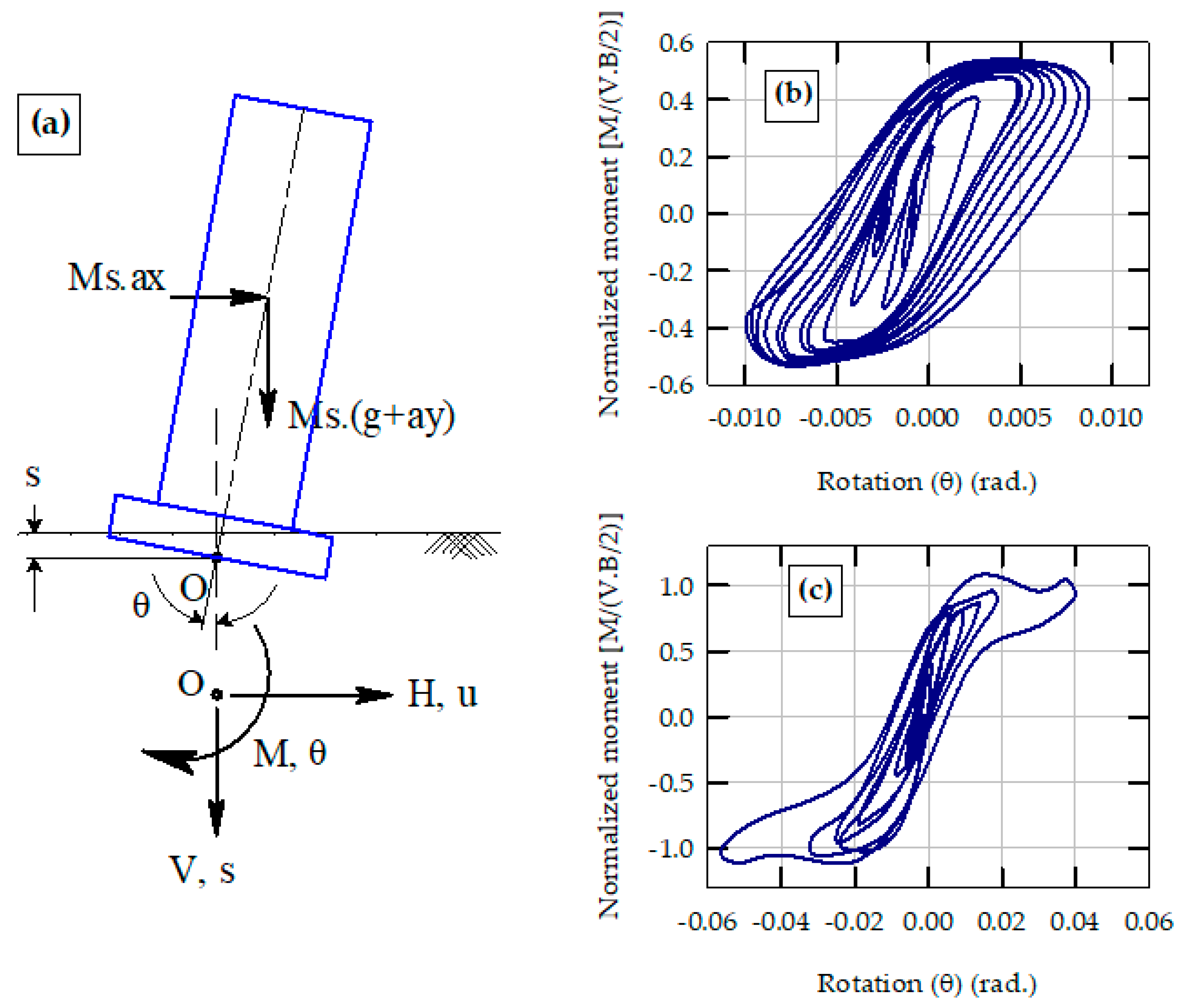
Figure 1. (a) Illustration of forces and displacements at soil–foundation interface of a rocking structure, and example experimental results for cyclic moment–rotation response of rocking foundations: (b) centrifuge experiment, A/Ac = 3.2 (FSv = 4), Cr = 0.17, and amax = 0.55 g; and (c) shake table experiment, A/Ac = 11.8 (FSv = 24), Cr = 0.31, and amax = 0.36 g.
Geotechnics 01 00024 g001
Figure 2. Variation (summary results) of normalized total seismic energy dissipation (NED) in foundation soil with Arias intensity of earthquake motion (Ia) and rocking coefficient (Cr) of soil–foundation system (experimental data from 140 centrifuge and shaking table model tests).
Geotechnics 01 00024 g002
Figure 3. Variation (summary results) of normalized total seismic energy dissipation (NED) in foundation soil with four of the input features used in machine learning models: A/Ac, h/B, Cr and amax/g (experimental data from 140 centrifuge and shaking table model tests).
Geotechnics 01 00024 g003
Figure 4. Initial split of experimental data for training (98 instances) and testing (42 instances) of machine learning models, showing the variation of NED with (a) Arias intensity and (b) peak horizontal acceleration of ground motion.
Geotechnics 01 00024 g004
Figure 5. Comparisons of weighted k-nearest neighbors regression model (KNN) predictions with experimental results for normalized seismic energy dissipation (NED) during: (a) training phase and (b) testing phase of the model.
Geotechnics 01 00024 g005
Figure 6. Comparisons of support vector regression model (SVR) predictions with experimental results for normalized seismic energy dissipation (NED) during: (a) training phase and (b) testing phase of the model.
Geotechnics 01 00024 g006
Figure 7. Comparisons of decision tree regression model (DTR) predictions with experimental results for normalized seismic energy dissipation (NED) during: (a) training phase and (b) testing phase of the model.
Geotechnics 01 00024 g007
Figure 8. Results of hyperparameter tuning of machine learning models: Variation of mean absolute percentage error (MAPE) during training and testing phases of the models with (a) number of nearest neighbors (k) in KNN model, (b) maximum depth of tree in DTR model, and (c) the value of penalty parameter “C” in SVR model.
Geotechnics 01 00024 g008
Figure 9. Comparison of model performances during training and testing phases of machine learning models: (a) mean absolute percentage error (MAPE) and (b) coefficient of determination (R2) (note: both figures share the same legend).
Geotechnics 01 00024 g009
Figure 10. Boxplots of mean absolute percentage errors (MAPE) of machine leaning models (testing error): (a) Repeated 5-fold cross validation and (b) repeated 7-fold cross validation (note: boxplots plot the median, 10th, 25th, 75th, and 90th percentiles of data along with the mean values (green triangles) and the extreme values (5th and 95th percentiles—red circles)).
Geotechnics 01 00024 g010
Table 1. Key statistical parameters of input features used in machine learning algorithms.
Input FeatureA/Ach/BCramax (g)Ia (m/s)
Range1.9–17.11.2–2.830.08–0.360.04–1.280.03–26.4
Mean8.171.890.240.432.31
Std. dev.4.270.530.080.264.37
Table 2. Coefficients of correlation between input features used in machine learning algorithms.
Input FeatureA/Ach/BCramax (g)Ia (m/s)
A/Ac1.0−0.390.660.13−0.18
h/B−0.391.0−0.86−0.11−0.2
Cr0.66−0.861.00.070.02
amax (g)0.13−0.110.071.00.34
Ia (m/s)−0.18−0.20.020.341.0
Publisher’s Note: MDPI stays neutral with regard to jurisdictional claims in published maps and institutional affiliations.