Article

Spatial–Temporal Analysis of PM2.5 Contamination, Thermal Pollution, and Population Social Backwardness in the Metropolitan Area of Mexico City


by
Monica Ballinas
*,
Bolívar Morales
and
Pablo López-Ramírez
Centro de Investigación en Ciencias de Información Geoespacial, A.C., Contoy 137, Col. Lomas de Padierna, Alcaldía Tlalpan, Ciudad de México CP 14240, Mexico
*
Author to whom correspondence should be addressed.
Geographies 2026, 6(1), 12; https://doi.org/10.3390/geographies6010012
Submission received: 29 November 2025 / Revised: 24 December 2025 / Accepted: 30 December 2025 / Published: 29 January 2026

Abstract

Atmospheric contamination and thermal pollution are two phenomena that impact negatively on the quality of life of residents in a city. Furthermore, exposure to these phenomena has a differential impact on socioeconomic strata, with the poorest being the most affected. Spatial and temporal analyses were conducted of PM2.5 pollution and air temperature, as well as socioeconomic variable. This characterization revealed that low-income people are more exposed to thermal pollution during the warm season with temperatures up to 32.6 °C, and to PM2.5 pollution with concentrations up to 205 µgm−3 during the cold season, focusing on the eastern part of the Metropolitan Area of Mexico City (MAMC). High temperatures can persist for up to 6 h, while PM2.5 concentrations can persist for up to 5 h. The social backwardness index is a fixed variable that can change in the long term and is related to thermal pollution. This study will allow us to understand social and environmental vulnerability and, thus, to develop an appropriate mitigation methodology for these two phenomena and their impact on human health, with special attention to environmental justice issues.

1. Introduction

In the Metropolitan Area of Mexico City (MAMC), there are two phenomena that affect human health, on the one hand, atmospheric pollution and on the other, the urban heat island (UHI). The UHI is a phenomenon in which the air temperature of the urban area is higher compared to the rural area [1,2,3,4,5]. The temperature increases due to the change in land use, which causes a redistribution and storage of solar energy [5]. The increase in temperature can negatively affect human thermal comfort and consequently causes a decrease in productivity and can lead to health problems causing respiratory, cardiovascular, and cerebrovascular diseases, mainly in the spring–summer season [6,7,8,9].
In addition, pollution by particles smaller than or equal to 2.5 μm (PM2.5), which are composed of sulfates and nitrates [10,11] and originate from power generation plants [12,13,14], dust, forest fires, vehicle emissions, wood burning, and industries [15,16], is considered one of the most harmful pollution particles to health [16,17,18], since it affects the respiratory tract [16,19,20,21], causes kidney inflammation, oxidative stress, cell death [16,22], cardiovascular diseases, and lung cancer [23,24].
MAMC population is exposed to these two atmospheric phenomena, because more than 14 Mg of PM2.5 are thrown into the air, with 41.7% being generated by mobile sources, 40% by area sources, 14.5% generated by point sources, and 3.8% by natural sources. Mobile sources are vehicles that operate with diesel (tractors, cargo vehicles, and buses), and area sources are open burning of solid waste [25].
Meanwhile, social backwardness is defined as a relative indicator of poverty [26], which means that there is the absence of at least one right for social development and insufficient income to acquire the goods and services that guarantee satisfaction of their needs [27]. One of the greatest inequalities in Mexico is the difference in the definition of environmental justice, as environmental degradation among social groups depends on their socioeconomic status and race [28,29,30].
Due to the exposure that urban residents of the MAMC experience to PM2.5 contamination and thermal pollution, an analysis was conducted showing the spatial distribution of these two phenomena in the metropolitan area, locating the sites with the highest concentration of these phenomena. This study also considers the socioeconomic status of the inhabitants of the MCMA, and therefore, this analysis demonstrates how PM2.5 and thermal pollution differentially impact the different socioeconomic strata, with the lowest-income groups being the most affected. The objective of this research was to determine the spatial distribution of PM2.5 and thermal pollution in the MAMC, and how the areas where inhabitants are vulnerable to these two phenomena, in addition to their economic and social vulnerability.

2. Materials and Methods

2.1. Study Area

The Metropolitan Area of Mexico City comprises an area of 3540 km2 [31,32], located at 19°03′–19° 54′ N and 98°38′–99°31′ W, and at an average elevation of 2240 m asl (Figure 1), with more than 21 million inhabitants [33]. The MAMC is made up of 16 municipalities in Mexico City, 60 municipalities in the State of Mexico and Tizayuca (a municipality in the State of Hidalgo) [34]. The expansion of the urban area has occurred further to the north mainly due to the easy and not-so-expensive access to housing, while in the southern area, there is still agricultural territory [35] and forest, where housing is more expensive. The area has a subtropical mountain climate, with an average annual precipitation of 748 mm which occurs mostly (94%) in the humid season (June–November), and the winds are light and predominately from the northeast. Extreme maximum and minimum temperatures are recorded between March and April (25 °C) and in January (5 °C), respectively [35]. In addition to this, the UHI is well established during the day, with an intensity of up to 10 °C [4,36].

2.2. Atmospheric Data

The PM2.5 data were obtained from the Automatic Atmospheric Monitoring Network (RAMA, its acronym in Spanish). Meteorological variables—air temperature (TA), relative humidity (RH), direction (Θ), and wind speed (WS)—were obtained from the Meteorological and Solar Radiation Network (REDMET, its acronym in Spanish), both from the Air Quality Monitoring Directorate of the Mexican Ministry of the Environment. Data is recorded every hour, daily, throughout the year. RAMA has 34 monitoring sites, and REDMET has 28 sites, distributed across the MAMC [37]. However, not all stations have available data, so at least 70% of the recorded data was selected (Table A1, Appendix A). From PM2.5, the monitoring system had 15 stations with information and for meteorological variable, 22 stations.
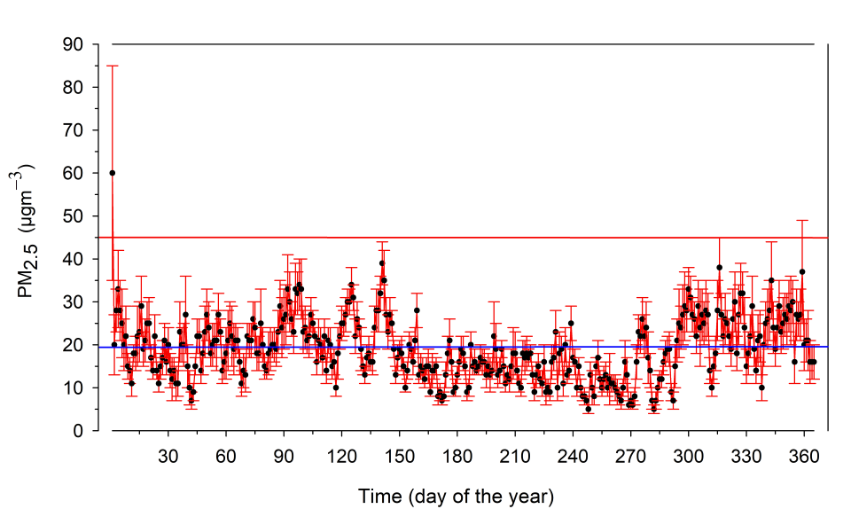
The PM2.5 analysis was carried out based on the definition made by the Mexican Regulations (NOM-025-SSA1-2021) [11], which specifies that exposure to a concentration of above 45 μgm−3 on average over 24 h is harmful (acute exposure).

2.3. Physiological Equivalent Temperature as an Index of Thermal Pollution

To determine the thermal pollution that generates thermal stress in the study area, an analysis of the physiological equivalent temperature (PET) was carried out. This index estimates human thermal perception through a categorization given for urbanites in the MAMC [5]. This index shows that when a limit of a thermal range is exceeded, the person enters thermal discomfort. The PET was calculated with the Rayman model, which incorporates meteorological data (WS, TA, RH, solar radiation), physical characteristics of people: height, weight, metabolism (activity), and gender [38]. Also, it incorporates the characteristics of the site (station height, sky view factor) and long-wave radiation, shadow duration, topography and obstacles, and urban structure [39] (Table A2, Appendix A).

2.4. Social Backwardness Index (SBI)

Social backwardness consists of rigorous theoretical and conceptual considerations given by an index and a grade, which are used as indicators of the social rights of the population in any area in Mexico [27]. This index includes current income per capita, average educational backwardness in the home, access to health services, access to social security, quality and spaces of housing, access to nutritious and quality food, degree of social cohesion, and degree of accessibility to paved roads, indicators that have been established by the Ley General de Desarrollo Social (current article 36). This law gives a multidimensional perspective of the deficiencies faced by the population, through a person’s income to satisfy their needs when they do not have at least some of their rights for social development guaranteed [27].
This index is classified into five degrees: very low, low, medium, high, and very high. It is presented at the AGEB level (basic geographic area). AGEBs are polygons that contain a small area with a maximum of 2500 inhabitants. Urban classification is made up of a set of blocks (from 1 to 50 blocks) that are delimited by streets, avenues, or other land use features such as industrial, residential or commercial, etc. [27].

2.5. Data Analysis

With the objective to understand the relationship between our three parameters, a geostatistical analysis of environmental variables (PM2.5 and TA) and their relationship with social backwardness in the MCMA was carried out. It was necessary to spatially link the point data from the monitoring stations with census territorial units (AGEB). This analysis will allow us to contextualize each point observation within a specific spatial unit, in this case a census polygon, which is key to incorporating sociodemographic information (such as the social backwardness index) at each monitoring point. It will also ensure the spatial consistency of the data, guaranteeing that the points are contained within the study area. It will also prepare the basis for multiscale analysis, where continuous variables (such as pollutants and temperature) can be analyzed based on territorial characteristics. To do this, the st_join() function from the sf package in R 4.4.1 software was applied to perform a point–polygon spatial union between the monitoring stations (POINT objects) and the AGEB polygons (MULTIPOLYGON objects). The operation assigns to each point the social lag value corresponding to the polygon in which it is located.
With the purpose of, it will facilitate visualization and geographic analysis of related data of different natures (environmental and sociodemographic); this type of analysis is recommended in studies of environmental exposure and territorial justice, where spatiality is a central dimension. Likewise, it was performed a multifactor analysis of variance (ANOVA), constructed various tests to determine which factors have a statistically significant effect on, and also test significant interactions amongst them. To make the interpolations and show the spatial distribution, Moran’s I test was applied as well.

3. Results

3.1. Urban Temperature

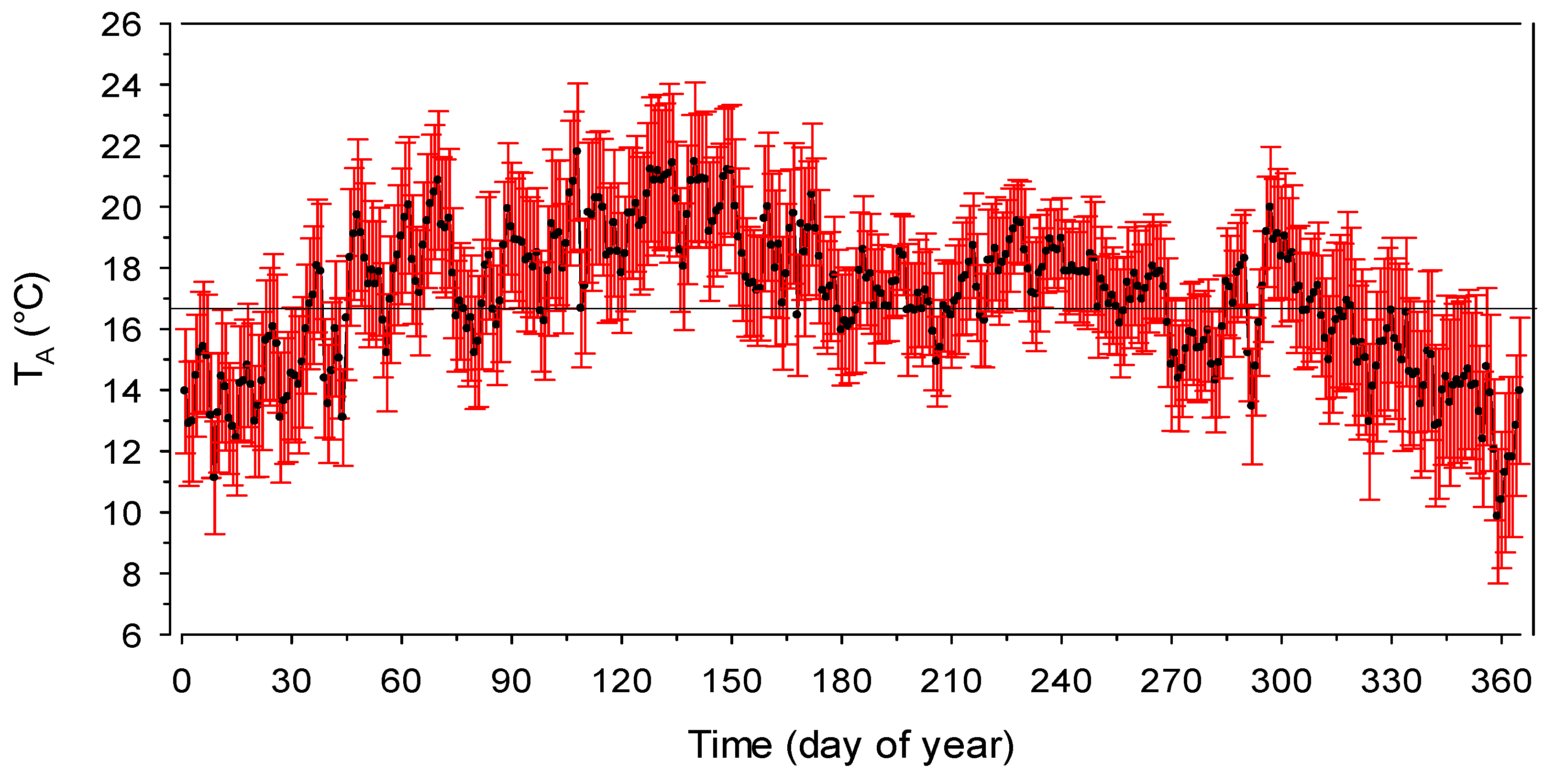
Figure 2 shows the behavior of the average daily air temperature for the year 2022 in the entire metropolitan area. The annual average was 16.9 °C, with May being the warmest month with 20.3 °C and December the coldest (13.6 °C). The highest temperature recorded was 32.6 °C on 9 May at 16:00 LST at the SAC station, and the lowest recorded temperature was −1.8 °C on 1 March at 08:00 LST in AJU. The temperature on 1 January fluctuated from −0.1 °C (minimum) to 26.5 °C (maximum) [37].

3.2. PM2.5 Concentration

Figure 3 shows the behavior of PM2.5 pollution, corresponding to the year 2022, with the maximum value allowed over 24 h in the whole metropolitan area. It is observed that, when considering the year 2022, the inhabitants of the MAMC were exposed to PM2.5 pollution for at least 174 days, being the fact that the average level of this pollutant exceeded for most of the year. The months of March, April, May, November, and December are the ones that reach the highest number of days in the month, above the allowed average (21, 23, 22, 23, and 25 days, respectively).
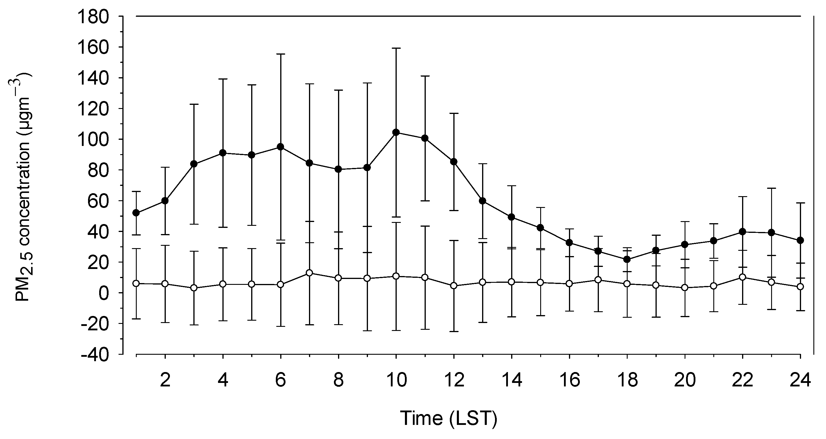
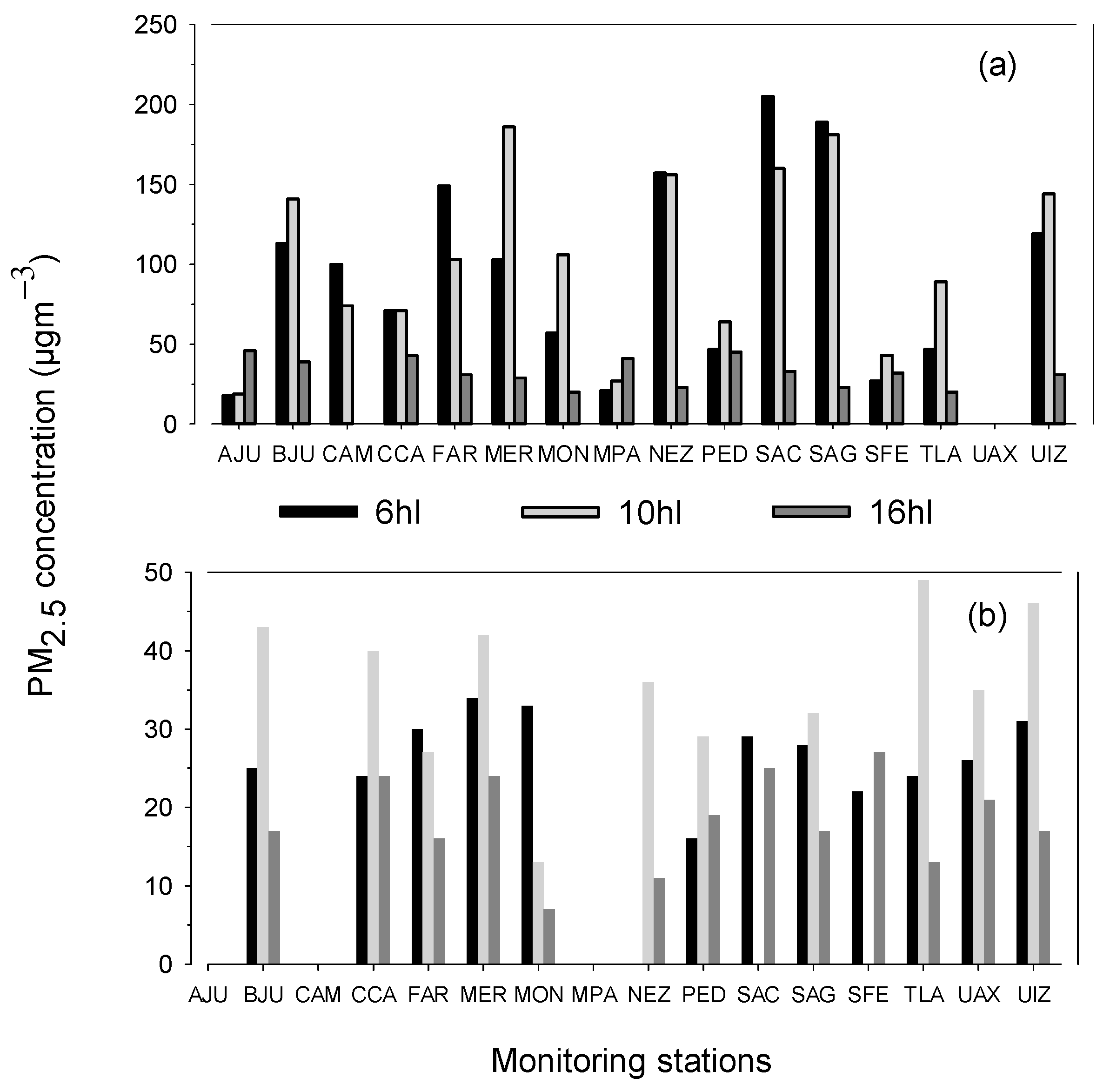
Average trend of hourly concentrations of PM2.5 in the entire metropolitan area are shown in Figure 4. It is evident that on 1 January 2022, very high averages are reported, well above 45 µgm−3 from 00:00 local time (LST) until 14:00–15:00 LST; in general, these are high values and take longer to disappear, compared to the values monitored on 9 May. In May, average values are around 10 μgm−3. It is also notable that in January, PM2.5 concentrations were much more variable in the metropolitan area than in May. Although it is at 06:00 LST when the highest concentration is recorded in an area such as SAC (205 μgm−3), it is observed that in the period of 10:00–11:00 LST values occur too, compared to the early morning resulting in 09 of 15 monitoring stations (Figure 5) with this behavior. While in January the highest concentrations are recorded around 06:00 LST, in May, they are recorded at 10:00 LST.

3.3. Thermal Pollution

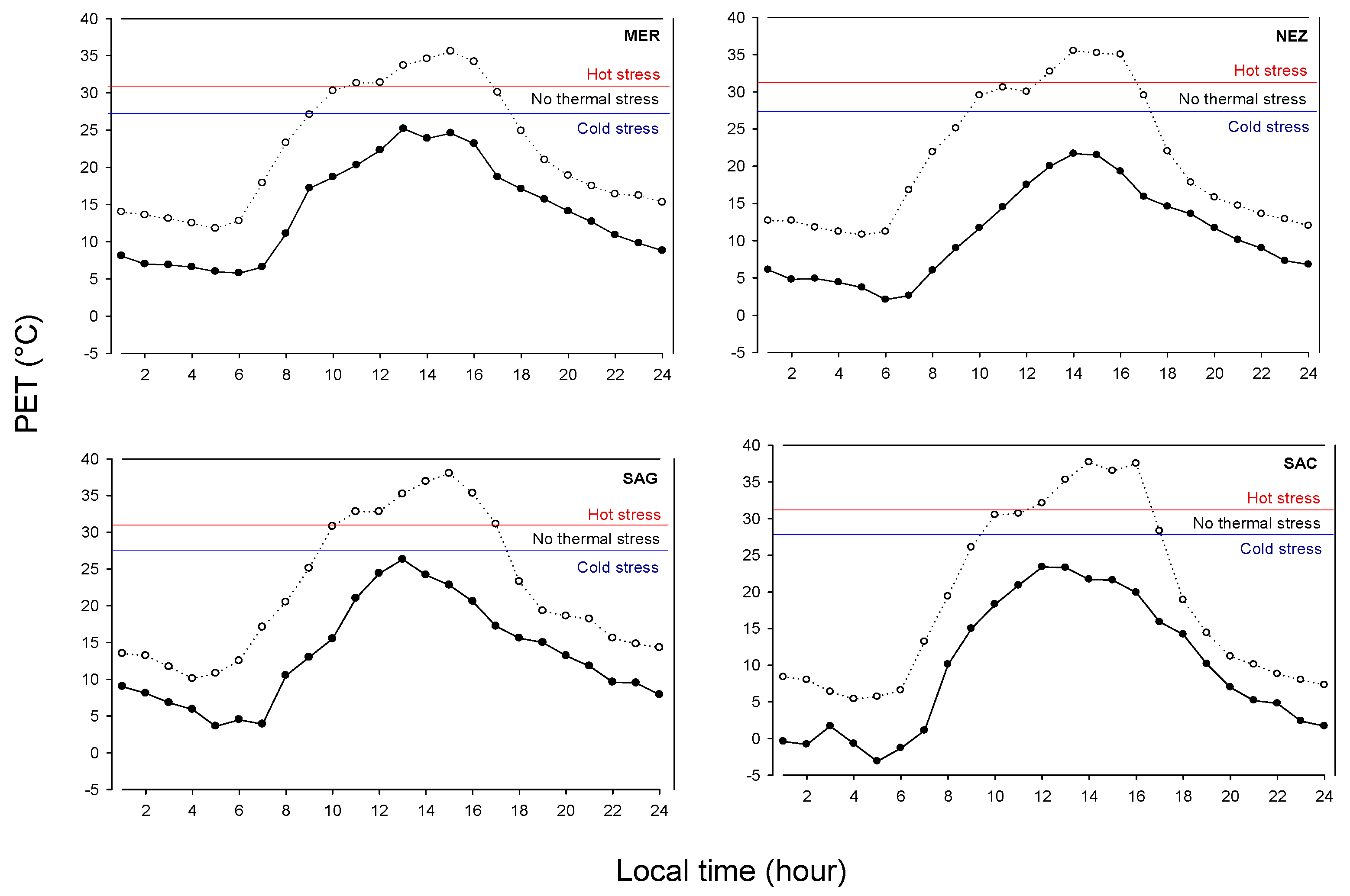
The excess air temperature that makes up the UHI can be considered as a form of thermal pollution due to the thermal stress that a person can experience in a location due to excess heat [4,36]. The PET coincides with the highest concentration of PM2.5 on 1 January (cold dry season) and the highest temperatures recorded 9 May (warm dry season) throughout the day for SAG, SAC, NEZ, and MER in 2022.
It is worth noting that in May, MER and SAG are the areas where people can experience six and seven hours of heat stress, respectively. MER counted at least two hours of thermal comfort, but SAG did not reach the thermal comfort classification at any time (Figure 6).

3.4. Interpolation Validation

The horizontal distributions of the studied variables were constructed using interpolations with the lowest possible error. In this case, Gaussian Kriging—ordinary was used (TA January RSME = 2.5; TA May RMSE = 1.7; PM2.5 January RMSE = 37.8; PM2.5 May RSME = 5.9). These interpolations were displayed in a geographic information system [40].
There is a strong contrast between the studied dates. In January, a high deviation of PM2.5 concentrations was noted, with an average (Avg) and standard deviation (SD) of 99.6 and 67 µgm−3, respectively, indicating variable and possibly severe pollution (>200 µgm−3) but low temperatures (Avg = 9.1 °C; SD = 3.2 °C). However, in May, PM2.5 concentrations were lower at all stations (<50 µgm−3; Avg 17.0 µgm−3; SD = 6.0 µgm−3), with a low deviation indicating clean air. Nevertheless, high dispersion and high temperatures are present (TA Avg = 30.5 °C; SD = 1.3 °C) compared to January, but no extreme levels of pollution are observed; the distribution is more homogeneous.
Moran’s I test for PM2.5 (I = 0.2051, p = 0.0121) on the two dates studied indicates that in January, there is a positive and significant spatial autocorrelation. This shows that PM2.5 pollution clusters according to the concentration of the pollution degree by season. In May, Moran’s I is negative, and the p = 0.4637 is not significant, indicating insufficient evidence to assert spatial autocorrelation. PM2.5 values are randomly distributed across the metropolitan area. This is probably due to improved atmospheric dispersion (such as wind, see Figure 7), as all stations have similar concentration values, resulting in more homogeneous conditions.
Regarding air temperature, global spatial autocorrelation analysis revealed a strong and significant spatial dependence. In January, Moran’s I was 0.726 (p < 0.001), while in May it reached 0.789 (p < 0.001). In January, the cross-validation revealed a mean error (0.008) that was practically zero. However, in May, the mean error (−0.086) is slightly negative, but somewhat more dispersed than in January.
The interaction between factors (PM2.5 and TA) was different between seasons for PM2.5 (F(95,191) = 0.90 (p = 0.6899)). For TA, differences were found both in site and time, with F(95,191) = 2.66 (p = 0.000). This means that there is a strong contrast between scenarios, in winter experiences higher concentrations of pollutants but lower temperatures, and in spring, temperatures increase but PM2.5 concentrations decrease due to the greatest dispersion of pollutants occurring during the warm season in the MCMA.

3.5. Urban Heat Island and PM2.5 Concentration

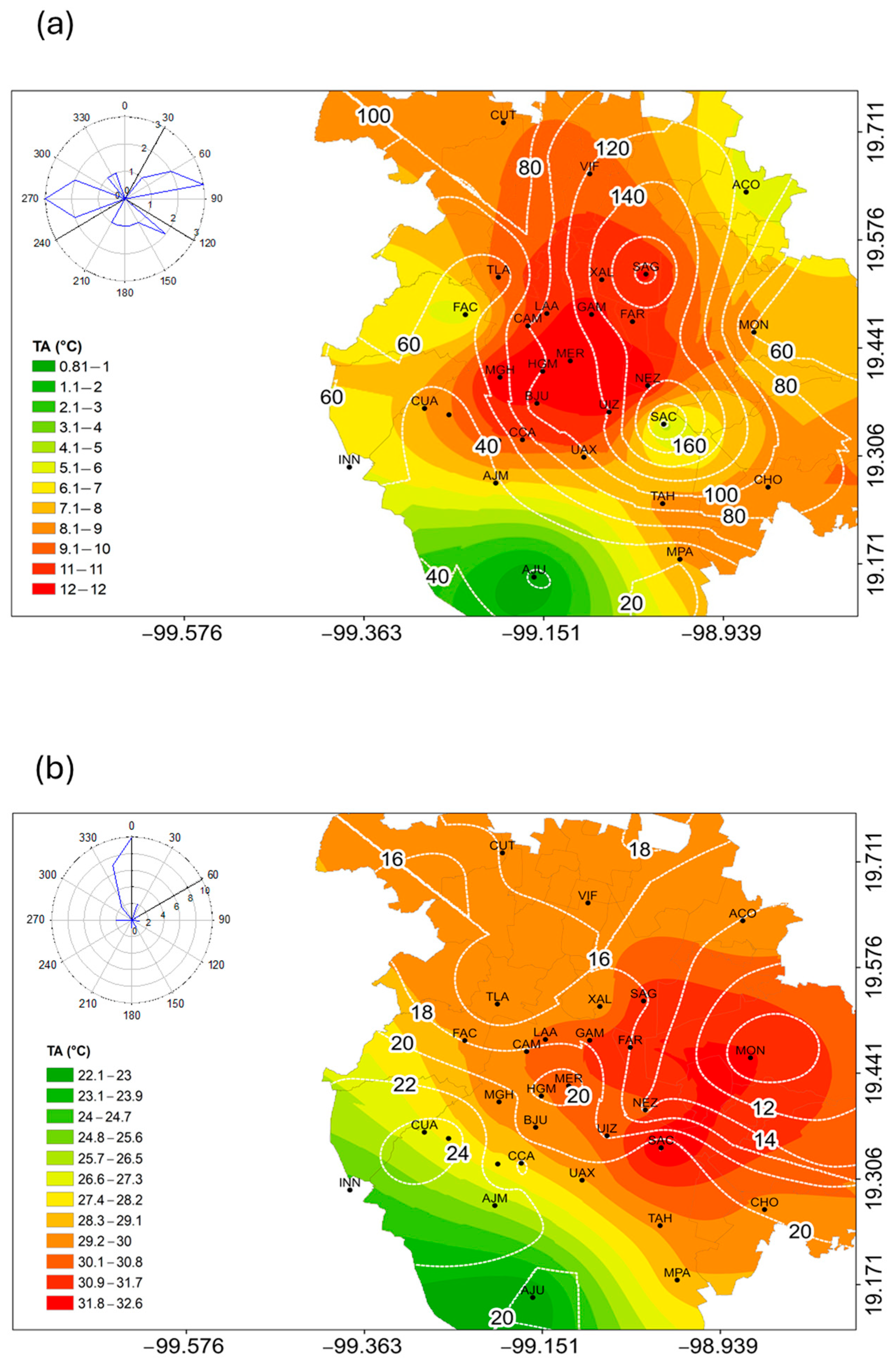
Figure 7 shows the spatial analysis of the PM2.5 concentration and air temperature in the MAMC on 1 January (a) and 9 May (b) in 2022.
Two areas of high PM2.5 concentrations are observed in the southeast part of the metropolitan area; in the south, it is located the SAC station with 205 µgm−3, and in the northeastern located in the SAG station area with 189 µgm−3. At these stations, the temperature was 5.1 °C and 11.1 °C for SAC and SAG, respectively. The heat island presented on 1 January indicates a magnitude ΔT(U-R) = 11 °C (Figure 7a). Meanwhile, in Figure 7b it corresponds to the warmest day: 9 May at 16:00 LST. It is observed that PM2.5 is found throughout the valley, located in the west in SFE with 27 µgm−3, followed by SAC in the east with 25 µgm−3 and in the city center in MER and in the south in CCA with 24 µgm−3.
On 1 January 2022, at 06:00 LST (Figure 7a), the minimum temperature was 0.8 °C at the AJU station, and the maximum temperature at MER was 11.9 °C. The UHI temperature distribution (TU-R) shows that because AJU is located at an altitude of 2930 m asl and MER is at 2245 m asl, and if the vertical temperature gradient and the configuration of areas, it was expected that TU-R would be of great magnitude, as it was in this case, with a difference of up to 11.1 °C. Therefore, when considering a station within the city that will have an area with land use conditions different from MER (semi-rural or semi-urban), such as ACO (2198 m asl), the intensity of the UHI was TU-R = 6 °C.
The air temperature distribution shows that on 1 January (Figure 7a), the lowest temperature was 0.8 °C in AJU and 11.9 °C in MER (ΔT = 11.1 °C). An archipelago with three islands is observed, the first island corresponding to the area between MER, NEZ, and UIZ, which exhibit a temperature of 11.9 °C, 11.5 °C, and 11.1 °C, respectively (average TA = 11.5 °C). In MGH the temperature was 11.9 °C and 11.1 °C in UAX. On 9 May (Figure 7b), the recorded temperatures were 22.1 °C in AJU and 32.6 in SAC, with a ΔT = 10.5 °C. There is an archipelago made up of two well-marked islands in the MON, FAR, and SAG area, where the temperatures were 31.8 ° C, 31.7 °C and 31.5 °C, respectively (average TA = 31.6 °C); the second island made up of the SAC, TAH, and CHO stations, with 32.6 °C, 29.3 °C, and 29.6 °C, respectively (average TA = 30.5 °C).

3.6. Horizontal Distribution of Social Backwardness Index

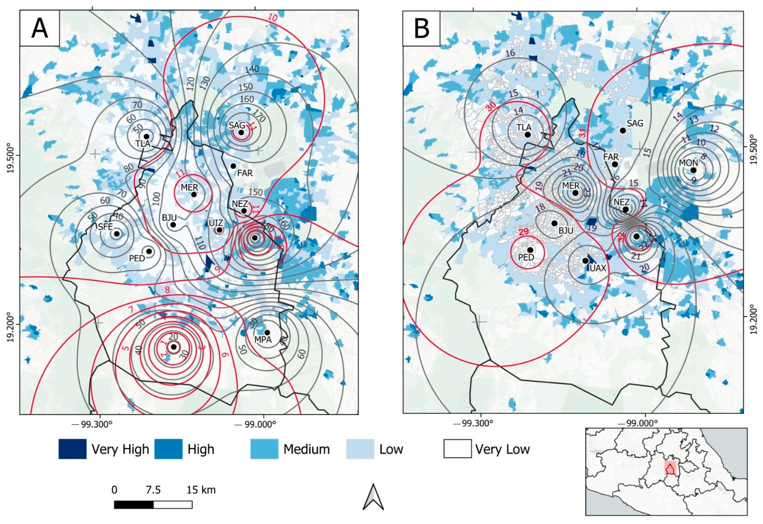
Figure 8 shows the intersection of the horizontal distribution of temperature (heat island) and the SBI. It is important to note that the five levels of lag are distributed throughout the metropolitan area; however, the highest index (medium–very high) is generally distributed throughout the metropolitan area, but is more concentrated in the eastern part of the city, with the greatest presence in the northeast quadrant, while the lowest indices (medium–very low) are distributed throughout the metropolitan area, but with a greater presence in the western zone and in the southwest quadrant. Meanwhile, on the one hand, the temperature distribution at 16:00 LST shows the classic heat island placed towards the east, with a center of 32 °C, coinciding with areas of higher SBI values that range from very high to medium, but it extends to the 30 °C isoline. On the other hand, low temperatures coincide with areas of lower social backwardness (medium to very low).

3.7. SBI and Environmental Variables

In January, there is no significant association between PM2.5 pollution and SBI levels (ρ = 0.006; p < 0.6087), while in May there is; although it is weak, it is significant, with high levels of SBI (ρ = −0.060; p < 0.001), and PM2.5 pollution tending to be slightly lower. This implies that urban areas with fewer social disadvantages have slightly higher levels of pollution, while in the outskirts with greater social disadvantage, the concentration of this pollutant is lower. However, it should be noted that the association (ρ) is very low, so the effect is statistically detectable but not relevant in magnitude. This indicates that other spatial and environmental factors (wind, TA, or other emission sources) are more determining than the level of marginalization.
Regarding TA, ρ shows a moderate negative correlation, meaning that the greater SBI is, the lower the temperatures tend to be in January (ρ = −0.366; p < 0.001) (<TA, >SBI; therefore, >TA, <SBI). This relationship could be linked to the geographic location of the AGEBs, where the sectors with the greatest social backwardness tend to be located in peripheral and higher-altitude areas. While in May, the relationship is weak, although statistically significant (ρ = 0.045; p = 0.0002), and the strength of the relationship is practically zero. This indicates that temperature is distributed evenly across the different levels of SBI.

4. Discussion

It is noteworthy that the high levels of PM2.5 and thermal pollution are concentrated in areas with medium to higher degree of social backwardness, while in areas with a lower degree of social backwardness, these two factors are not as intense. This can be explained in part by the fact that Mexico City residents with high socioeconomic levels settled in areas with a more humid climate and therefore with more vegetation and more expensive, while those with low resources settled in the drier area, where xerophilous scrub and grasslands dominate. Roughly speaking, a separation of social backwardness is observed in the metropolitan area that goes from the southeast to the northwest. This is an example of possible gentrification in the MAMC. Broadly speaking, a separation of social backwardness is observed, going from the southeast to the northwest, with some exceptions; this separation is given by the location of the following meteorological stations: MPA, TAH, UIZ, MER, CAM, and TLA.
These spatial analyses are consistent with those obtained in 1968 by Dolores Riquelme [41], who found that the southern part of the MCMA had the least pollution due to its low industrialization and high vegetation cover. This is coupled with the fact that the residential areas were more open and had tree-lined gardens, compared to the northern and eastern areas, where the lots were smaller, lacking green spaces, and buildings crowded together, where proletarian-style dwellings were found. These areas were also affected by dust storms from the former Lake Texcoco.
The coincidence of high rates of thermal pollution and PM2.5 in areas with high degree of social backwardness can have a greater impact on cardiovascular disease and mortality in these low-income groups [42,43,44]. In the long term, for every 10 µgm−3 increase in fine particle concentration, the risk of mortality from lung cancer and cardiopulmonary diseases increases [13]. Furthermore, although exposure to air pollution increases with age, a high mortality rate has been found in Africa and South Asia in children under five years old, of which 13.8% of global mortality is due to cardiovascular diseases, 21.4% corresponds to children [44]. Additionally, diabetes can be exacerbated by high concentrations, and 4.2 × 10⁶ deaths worldwide are correlated with PM2.5 [45].
The combination of PM2.5 and UHI, in which high temperatures over 32 °C can stand out, poses a high risk to health in the MAMC. When these temperatures are reached, people experience thermal stress that can lead to dehydration or heat exhaustion, and subsequently heat stroke can occur, which increases mortality. Above 40 °C, hyperthermia and brain damage can occur [46], or high temperatures can also affect hospitalization rates for cardiovascular and respiratory diseases [8], thereby causing death [47]. Thus, for vulnerable groups with a high social gap, these effects are enhanced and coincide with what was found in the United States, in which this sector of the population is more exposed to PM2.5 [48], and if high temperatures are considered, the risk of mortality increases. Thus, the area with the highest social disadvantages coincides with high temperatures due to UHI and high concentrations of PM2.5, resulting in a highly vulnerable population.
People from the poorest groups not only face economic hardship, but also limited access to healthcare, not only for the low number of health facilities and the low level of equipment in them, but also because of their accessibility. These social inequalities mean that cities are outside the framework of sustainable development, which places the population at risk of being exposed to pollution [49]. Therefore, it must be emphasized that cities in general are vulnerable areas due to the loss of biodiversity for the land use changes and the construction of urban infrastructure, which leads to an environmental degradation, entirely spatial, with both in horizontal and vertical aspects. This leads to a global environmental crisis, increasing cases of social injustice, which poses a threat to the population in their health problems linked to pollution [50,51]. In addition to the fact that the burning of fireworks during celebrations releases particulate matter into the atmosphere, exacerbating PM2.5 pollution, thermal inversions are more persistent during the colder months, concentrating PM2.5 pollution in the lower atmosphere. Furthermore, lower wind speeds prevent pollution from dispersing (see compass rose in Figure 7). This can be observed in Figure 5, where these concentrations persist until 11:00 LST.

5. Conclusions

The environmental impact of the MAMC is not only very high, but the environmental justice that should prevail in a city of this size is also not being achieved. Urban residents, in addition to experiencing a high degree of social backwardness due to a lack of resources and access to basic necessities, are also suffering from the significant impact of PM2.5 contamination and heat pollution. In addition to the fact that there is a large coincidence where low-income population was displaced by gentrification, they went to live on low-cost land. These deficiencies could lead to the Mexican population probably not having the necessary information to mitigate these environmental impacts, assuming that, by affecting their health, they could not have a good quality of life and that this is not only due to the economic aspect. It is important to note that, regardless of social class, the population of MAMC is not exempt from suffering the effects of thermal pollution and PM2.5 contamination. However, vulnerability is greater for the population at a medium to very high level of social backwardness (SBI), since they do not have the resources or the conditions to access public health, which prevents them from minimizing the damage to their health.
It is necessary to take measures to counteract both PM2.5 pollution, which can be taken as an example of air pollution, as well as considering mitigate the urban heat island. Furthermore, it is essential to consider improving the economic environment for low-income residents of the MAMC.

Author Contributions

Conceptualization, M.B. and P.L.-R.; methodology, M.B. and B.M.; software, M.B. and B.M.; validation, M.B. and B.M.; formal analysis, M.B.; investigation, M.B.; resources, P.L.-R.; data curation, M.B. and B.M.; writing—original draft preparation, M.B.; writing—review and editing, M.B.; visualization, M.B.; supervision, M.B. and P.L.-R.; project administration, P.L.-R.; funding acquisition, P.L.-R. All authors have read and agreed to the published version of the manuscript.

Funding

This research was funded by Secretaría de Ciencia, Humanidades, Tecnología e Innovación (SECIHTI), under grant 1200/320/2022 MOD.ORD./09/2022 for the postdoctoral fellowship.

Institutional Review Board Statement

Not applicable.

Informed Consent Statement

Not applicable.

Data Availability Statement

The original contributions presented in this study are included in the article. Further inquiries can be directed at the corresponding author.

Acknowledgments

The first author thanks Alberto Porras for contributing to the first SBI and PM2.5 and TA map.

Conflicts of Interest

The authors declare no conflicts of interest.

Appendix A

Table A1. Land use classification and geographical characteristics of the stations belonging to the Automatic Atmospheric Monitoring Network, RAMA and REDMET [37].
StationsAbbreviationLand Use ClassificationMain CharacteristicsAltitude (m asl)LatitudeLongitude
AcolmanACOLow intensity semi-urban, surrounded by services and residential homes30% vegetation219819°38′08′′98°54′43′′
Ajusco *AJUSemi-rural surrounded by vegetation and grazing areaPlant cover293019°09′17′′99°09′45″
Benito Juárez *BJUHigh density urban area, surrounded by services, shops and apartmentsUrban with asphalt and concrete224619°22′14″99°09′35″
Camarones *CAMMedium density urban area, surrounded by shops and residential homesUrban with asphalt and concrete225419°28′06″99°10′11″
Centro de Ciencias de la Atmósfera *CCAMixed area with large buildings and open spacesUrban with asphalt and concrete227819°19′34″99°10′34″
ChalcoCHOLow density urban area, surrounded by shops and homesUrban with asphalt and concrete224319°16′01″98°53′10″
CuautitlánCUTLow density urban area with abundant green areasVegetation225019°43′20″99°11′55″
Fes AcatlánFACMixed area with large buildings and open landscapePavement, concrete and vegetation229919°28′57″99°14′37″
FES Aragón *FARMixed area with large buildings and open landscapePavement, concrete and vegetation223019°28′25″99°02′46″
Gustavo A. MaderoGAMMixed area with large buildings and open landscapePavement, concrete and vegetation222719°28′58″99°05′40″
Hospital General de MéxicoHGMHigh density urban area with tall buildings, shops and servicesPavement and concrete 225919°24′42″99°09′08″
Los LaurelesLAAMedium density urban area with houses and businessesPavement and concrete224219°29′02″99°08′50″
MercedMERMedium density urban area, houses, services and shopsPavement and concrete225019°25′29″99°07′11″
Miguel HidalgoMGHMedium density urban area, houses, services and shopsPavement and concrete236619°24′15″99°12′10″
Montecillo *MONSemi-rural mixed area with large buildings and crop fieldsPavement and plant cover206419°27′37″98°54′10″
Milpa Alta *MPASemi-rural area with few housesPavement and vegetation260019°10′37″98°59′25″
Nezahualcóyotl *NEZMedium density urban area, houses and businessesPavement and concrete224019°23′37″99°01′42″
Pedregal*PEDMedium density urban areaPavement and concrete232619°19′31″99°12′15″
Santiago Acahualtepec *SACMedium density urban area, houses and businessesPavement and concrete229019°20′44″99°00′34″
San Agustín *SAGMedium density urban areaPavement and concrete223919°31′59″99°01′49″
Santa Fe*SFEHigh density urban area with services and officesPavement and concrete259319°21′26″99°15′46″
TláhuacTAHLow density urban area, houses and businesses Pavement and concrete229719°14′47″99°00′38″
Tlanepantla *TLAMedium density urban area with houses and businessesPavement and concrete228319°31′45″99°12′17″
Universidad Autónoma Metropolitana XochimilcoUAX *Mixed area with large buildings and green areasPavement and concrete224619°18′16″99°06′13″
Universidad Autónoma Metropolitana Iztapalapa *UIZMixed area with large buildings and green areasPavement and concrete224519°21′39″99°04′26″
Villa de las FloresVIFMedium density urban area with houses and businessesPavement and concrete225019°39′30″99°05′48″
XalostocXALMedium density urban area with houses, shops and industriesPavement and concrete 226519°31′34″99°04′57″
* RAMA stations.
Table A2. PET ranges (°C), for an internal energy production of 120 W and a heat transfer through clothing of 0.49 clo, taking into consideration the acclimatization of people in Mexico City [5].
CategoryPET (°C)Thermal PerceptionGrade of Physiological Stress
0<18.7Very coldExtreme cold stress
118.8–20.9ColdStrong cold stress
221.0–25.5CoolModerate cold stress
325.6–27.5Slightly coolSlight cold stress
427.6–31.2ComfortableNo thermal stress
531.3–32.5Slightly warmSlight heat stress
632.6–33.5WarmModerate heat stress
7>33.6HotStrong heat stress
8>41Very hotExtreme heat stress

References

  1. Lee, D.O. Urban—Rural humidity differences in London. Int. J. Climatol. 1991, 11, 577–582. [Google Scholar] [CrossRef]
  2. Oke, T.R. The Heat Island of the Urban Boundary Layer: Characteristics, Causes and Effects. In Wind Climate in Cities, 1st ed.; Jack, C., Alan, G.D., Eric, J.P., Domingos, X.V., Eds.; Springer: Dordrecht, The Netherlands, 1995; Volume 277, pp. 81–107. [Google Scholar]
  3. Unger, J. Urban-rural air humidity differences in Szeged, Hungary. Int. J. Climatol. 1999, 19, 1509–1515. [Google Scholar] [CrossRef]
  4. Ballinas, M.; Barradas, V.L. The urban tree as a tool to mitigate the urban heat island in Mexico City: A simple phenomenological model. J. Environ. Qual. 2016, 45, 157–166. [Google Scholar] [CrossRef]
  5. Ballinas, M.; Morales-Santiago, S.I.; Barradas, V.L.; Lira, A.; Oliva-Salinas, J.G. Is PET an adequate index to determine human thermal comfort in Mexico City? Sustainability 2022, 14, 12539. [Google Scholar] [CrossRef]
  6. Seppanen, O.; Fisk, W.J.; Faulkner, D. Control of temperature for health and productivity in offices. ASHRAE Trans. 2004, 111, LBNL-55448. [Google Scholar]
  7. Tse, W.L.; So, A.T. The importance of human productivity to air-conditioning control in office environments. HVACR Res. 2004, 13, 3–21. [Google Scholar] [CrossRef]
  8. Michelozzi, P.; Accetta, G.; De Sario, M.; D’Ippoliti, D.; Marino, C.; Baccini, M.; Biggeri, A.; Anderson, R.; Katsouyanni, K.; Ballester, F.; et al. High temperature and hospitalizations for cardiovascular and respiratory causes in 12 European cities. Am. J. Respir. Crit. Care Med. 2009, 179, 383–389. [Google Scholar] [CrossRef]
  9. Kolokotsa, D.; Lilli, K.; Gobakis, K.; Mavrigiannaki, A.; Haddad, S.; Garshasbi, S.; Heshmat, H.; Paolini, R.; Konstantina, V.; Bartesaghi, D.; et al. Analyzing the impact of urban planning and building typologies in urban heat island mitigation. Buildings 2022, 12, 537. [Google Scholar] [CrossRef]
  10. Lee, J.T.; Kim, H.; Hong, Y.C.; Kwon, H.J.; Schwartz, J.; Christiani, D.C. Air pollution and daily mortality in seven major cities of Korea, 1991–1997. Environ. Res. 2000, 84, 247–254. [Google Scholar] [CrossRef] [PubMed]
  11. NOM-025-SSA1-2021; Salud Ambiental. Criterio para Evaluar la Calidad del Aire Ambiente, con Respecto a las Partículas Suspendidas pm10 y pm2.5. Valores Normados para la Concentración de Partículas Suspendidas PM10 y PM2.5 en el Aire Ambiente, Como Medida de Protección a la Salud de la Población Prefacio. Federale Overheid van Mexico: Mexico-Stad, Mexico, 2021. Available online: https://dof.gob.mx/nota_detalle.php?codigo=5633855&fecha=27/10/2021#gsc.tab=0 (accessed on 16 March 2023).
  12. Weagle, C.L.; Snider, G.; Li, C.; Van Donkelaar, A.; Philip, S.; Bissonnette, P.; Burke, J.; Jakson, J.; Latimer, R.; Stone, E. Global sources of fine particulate matter: Interpretation of PM2.5 chemical composition observed by SPARTAN using a global chemical transport model. Environ. Sci. Technol. 2018, 52, 11670–11681. [Google Scholar] [CrossRef]
  13. Pope Iii, C.A.; Burnett, R.T.; Thun, M.J.; Calle, E.E.; Krewski, D.; Ito, K.; Thurston, G.D. Lung cancer, cardiopulmonary mortality, and long-term exposure to fine particle air pollution. JAMA 2002, 287, 1132–1141. [Google Scholar] [CrossRef]
  14. Murray, C.J.; Aravkin, A.Y.; Zheng, P.; Abbafati, C.; Abbas, K.M.; Abbasi-Kangevari, M.; Abd-Allah, F.; Abdelalim, A.; Abdollahi, M.; Abdollahpour, I.; et al. Global burden of 87 risk factors in 204 countries and territories, 1990–2019: A systematic analysis for the Global Burden of Disease Study 2019. Lancet 2020, 396, 1223–1249. [Google Scholar] [CrossRef]
  15. Cho, C.C.; Hsieh, W.Y.; Tsai, C.H.; Chen, C.Y.; Chang, H.F.; Lin, C.S. In vitro and in vivo experimental studies of PM2.5 on disease progression. Int. J. Environ. Res. 2018, 15, 1380. [Google Scholar] [CrossRef]
  16. Yang, L.; Li, C.; Tang, X. The impact of PM2.5 on the host defense of respiratory system. Front. Cell Dev. Biol. 2020, 8, 91. [Google Scholar] [CrossRef]
  17. Pinkerton, K.E.; Green, F.H.; Saiki, C.; Vallyathan, V.; Plopper, C.G.; Gopal, V.; Hung, D.; Bahne, E.D.; Lin, S.S.; Ménache, M.G.; et al. Distribution of particulate matter and tissue remodeling in the human lung. Environ. Health Perspect. 2000, 108, 1063–1069. [Google Scholar] [CrossRef] [PubMed]
  18. Schulze, F.; Gao, X.; Virzonis, D.; Damiati, S.; Schneider, M.R.; Kodzius, R. Air quality effects on human health and approaches for its assessment through microfluidic chips. Genes 2017, 8, 244. [Google Scholar] [CrossRef]
  19. Feng, S.; Gao, D.; Liao, F.; Zhou, F.; Wang, X. The health effects of ambient PM2.5 and potential mechanisms. Ecotoxicol. Environ. Saf. 2016, 128, 67–74. [Google Scholar] [CrossRef] [PubMed]
  20. Ge, E.; Lai, K.; Xiao, X.; Luo, M.; Fang, Z.; Zeng, Y.; Ju, H.; Zhong, N. Differential effects of size-specific particulate matter on emergency department visits for respiratory and cardiovascular diseases in Guangzhou, China. Environ. Pollut. 2018, 43, 336–345. [Google Scholar] [CrossRef]
  21. Zheng, X.-Y.; Ding, H.; Jiang, L.-N.; Chen, S.-W.; Zheng, J.-P.; Qiu, M.; Zhou, Y.-X.; Chen, Q.; Guan, W.-J. Association between air pollutants and asthma emergency room visits and hospital admissions in time series studies: A systematic review and meta-analysis. PLoS ONE 2015, 10, e0138146. [Google Scholar] [CrossRef]
  22. Xu, W.; Wang, S.; Jiang, L.; Sun, X.; Wang, N.; Liu, X.; Yao, X.; Qiu, T.; Zhang, C.; Li, J.; et al. The influence of PM2.5 exposure on kidney diseases. Hum. Exp. Toxicol. 2022, 41, 09603271211069982. [Google Scholar] [CrossRef]
  23. Pun, V.C.; Kazemiparkouhi, F.; Manjourides, J.; Suh, H.H. Long-term PM2.5 exposure and respiratory, cancer, and cardiovascular mortality in older US adults. Am. J. Epidemiol. 2017, 186, 961–969. [Google Scholar] [CrossRef]
  24. Wang, C.; Tu, Y.; Yu, Z.; Lu, R. PM2.5 and cardiovascular diseases in the elderly: An overview. Int. J. Environ. Res. Public Health 2015, 12, 8187–8197. [Google Scholar] [CrossRef]
  25. SEDEMA (Secretaría del Medio Ambiente de la Ciudad de México). Red de Meteorología y Radiación Solar. Ciudad de México. Available online: https://aire.cdmx.gob.mx (accessed on 18 September 2023).
  26. Maldonado, F.J.B.; Meza, M.V.G. El rezago social en áreas metropolitanas de México. Estud. Econ. 2013, 28, 265–297. [Google Scholar] [CrossRef]
  27. Consejo Nacional de Evaluación de la Política de Desarrollo Social (CONEVAL). Metodología para la Medición Multidimensional de la Pobreza en México (Tercera Edición). Available online: https://www.coneval.org.mx/InformesPublicaciones/InformesPublicaciones/Documents/Metodologia-medicion-multidimensional-3er-edicion.pdf (accessed on 12 February 2023).
  28. Laurian, L. Environmental injustice in France. J. Environ. Plan. Manag. 2008, 51, 55–79. [Google Scholar] [CrossRef]
  29. Laurian, L.; Funderburg, R. Environmental justice in France? A spatio-temporal analysis of incinerator location. J. Environ. Plan. Manag. 2014, 57, 424–446. [Google Scholar] [CrossRef]
  30. Lome-Hurtado, A.; Touza-Montero, J.; White, P.C.L. Environmental injustice in Mexico City: A spatial quantile approach. Expo. Health 2020, 12, 265–279. [Google Scholar] [CrossRef]
  31. Sedesol-Conapo-Inegi (Secretaría de Desarrollo Social-Consejo Nacional de Población—Instituto Nacional de Estadística y Geografía). Delimitación de las Zonas Metropolitanas de México 2015. Available online: https://www.gob.mx/cms/uploads/attachment/file/305634/Delimitacion_Zonas_Metropolitanas_2015.pdf (accessed on 8 November 2023).
  32. Espejel Mena, J. The Metropolitan Zone of the Valley of Mexico: Formal arrangements and fragmentation. Econ. Soc. Territ. 2019, 19, 241–271. [Google Scholar] [CrossRef]
  33. Procuraduría Ambiental y del Ordenamiento Territorial de la Ciudad de México (PAOT). Mexico City: Condiciones Geográficas de la Zona Metropolitana de la Ciudad de México. Available online: https://paot.org.mx/centro/inegi/amdf2000/cap2.pdf (accessed on 15 February 2024).
  34. Zaragoza Badillo, J.; Guzmán, J.R. Economía, crecimiento urbano y el cambio climático local en la Zona Metropolitana del Valle de México. Inter Discip. 2023, 11, 311–332. [Google Scholar] [CrossRef]
  35. INEGI (Instituto Nacional de Estadística y Geografía). Available online: https://www.inegi.org.mx (accessed on 4 December 2023).
  36. Ballinas, M. Mitigación de la Isla de Calor Urbana a Partir de la Vegetación Arbórea. Master’s Thesis, Centro de Ciencias de la Atmósfera-Instituto de Ecología, UNAM, Ciudad de México, Mexico, 2011. [Google Scholar]
  37. SEDEMA (Secretaría del Medio Ambiente de la Ciudad de México). Inventario de Emisiones de la Zona Metropolitana del Valle de México 2020. Dirección General de Calidad del Aire, Dirección de Proyectos de Calidad del Aire. Available online: https://www.sedema.cdmx.gob.mx/ (accessed on 20 October 2024).
  38. Matzarakis, A.; Mayer, H.; Iziomon, M.G. Applications of a universal thermal index: Physiological equivalent temperature. Int. J. Biometeorol. 1999, 43, 76–84. [Google Scholar] [CrossRef]
  39. Matzarakis, A.; Rutz, F.; Mayer, H. Modelling radiation fluxes in simple and complex environments—Application of the RayMan model. Int. J. Biometeorol. 2007, 51, 323–334. [Google Scholar] [CrossRef]
  40. ArcGis Plataforma Geoespacial. Available online: https://www.esri.com (accessed on 18 September 2024).
  41. Riquelme, D. Microclimas del área metropolitana de la Ciudad de México. Anu. Geogr. 1968, 8, 103–105. [Google Scholar]
  42. Lelieveld, J.; Pozzer, A.; Pöschl, U.; Fnais, M.; Haines, A.; Münzel, T. Loss of life expectancy from air pollution compared to other risk factors: A worldwide perspective. Cardiovasc. Res. 2020, 116, 1910–1917. [Google Scholar] [CrossRef] [PubMed]
  43. Barrows, G.; Garg, T.; Jha, A. The Health Costs of Coal-Fired Power Plants in India; Working Paper; Center for Effective Global Action, UC Berkeley: Berkeley, CA, USA, 2019. [Google Scholar]
  44. Rentschler, J.; Leonova, N. Global air pollution exposure and poverty. Nat. Commun. 2023, 14, 4432. [Google Scholar] [CrossRef] [PubMed]
  45. Münzel, T.; Gori, T.; Al-Kindi, S.; Deanfield, J.; Lelieveld, J.; Daiber, A.; Rajagopalan, S. Effects of gaseous and solid constituents of air pollution on endothelial function. Eur. Heart J. 2018, 39, 3543–3550. [Google Scholar] [CrossRef]
  46. Luber, G.; McGeehin, M. Climate change and extreme heat events. Am. J. Prev. Med. 2008, 35, 429–435. [Google Scholar] [CrossRef] [PubMed]
  47. Hajat, S.; Kovats, R.S.; Lachowycz, K. Heat-related and cold-related deaths in England and Wales: Who is at risk? Occup. Environ. Med. 2007, 64, 93–100. [Google Scholar] [CrossRef]
  48. Bell, M.L.; Ebisu, K. Environmental inequality in exposures to airborne particulate matter components in the United States. Environ. Health Perspect. 2012, 120, 1699–1704. [Google Scholar] [CrossRef]
  49. Chancel, L. Insountenables Inégalités: Pour une Justice Sociale et Environnementale; Fuhem Ecosocial: Madrid, Spain; Les Petits Matins: Paris, France, 2021. [Google Scholar]
  50. Temper, L.; del Bene, D.; Martinez-Alier, J. Mapping the frontiers and front lines of global environmental justice: The EJAtlas. J. Polit. Ecol. 2015, 22, 255–278. [Google Scholar] [CrossRef]
  51. Venegas-Sahagún, B.A.; Gran-Castro, J.A. Injusticia ambiental y violaciones de los derechos humanos en Jalisco, México. ÍCONOS. Rev. Cienc. Soc. 2023, 77, 197–216. [Google Scholar] [CrossRef]
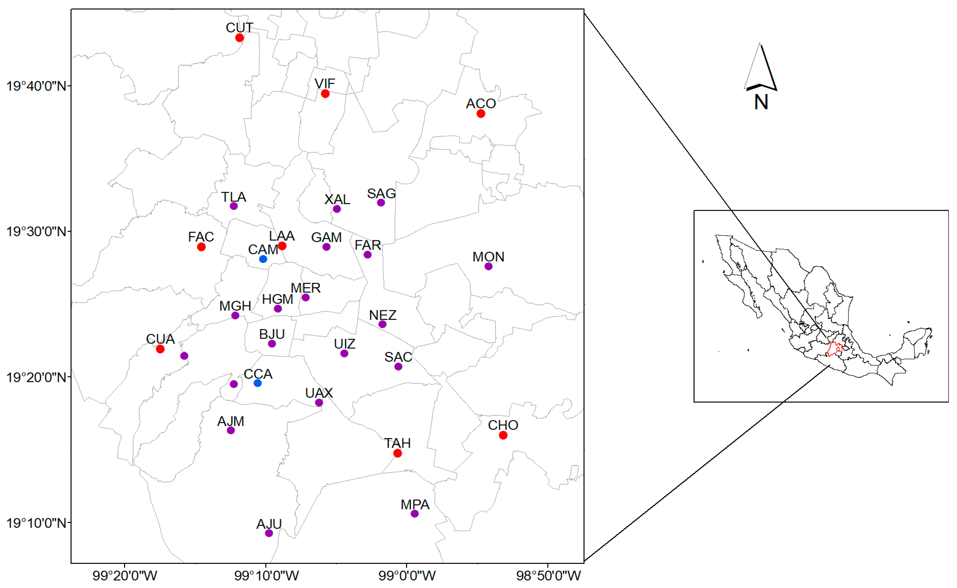
Figure 1. Location of the Metropolitan Area of Mexico City showing the distribution of the monitoring stations for PM2.5 particles and meteorological variables belonging to the Automatic Atmospheric Monitoring Network (blue circle, RAMA) and the Meteorological and Solar Radiation Network (red circle, REDMET), respectively. The purple circle corresponds to the stations that monitor the two variables studied together (PM2.5 and meteorological variables).
Geographies 06 00012 g001
Figure 2. Daily air temperature in the year 2022, corresponding to the 22 stations distributed in the MAMC. The solid line corresponds to the annual average. Daily averages and standard deviations are shown.
Geographies 06 00012 g002
Figure 3. Trend of PM2.5 average concentration over 24 h in the year 2022 in the whole metropolitan area. The red continuous line corresponds to the 45 µgm−3 according to the NOM-025-SSA1-2021. The blue continuous line corresponds to the annual mean 19 µgm−3 (SD = 7 µgm−3; n = 5024). Daily averages and standard deviations are shown.
Geographies 06 00012 g003
Figure 4. Average trend of hourly of PM2.5 concentration at the 15 monitoring stations, corresponding to 1 January (closed symbols) and 9 May (open symbols), 2022, in MAMC. Hourly averages and standard deviations are shown.
Geographies 06 00012 g004
Figure 5. PM2.5 concentration recorded on 1 January (a) and on 9 May (b) 2022 at 16 metropolitan stations distributed in the whole MAMC at different times of the day (06:00, 10:00, and 16:00 LST).
Geographies 06 00012 g005
Figure 6. PET trends during 1 January (closed symbols) and 9 May (open symbols) of 2022. The different classes of thermal perception are shown.
Geographies 06 00012 g006
Figure 7. PM2.5 (µgm−3, white isolines) and TA (°C, chorochromatic) spatial distributions recorded on (a) 1 January at 06:00 LST and (b) 9 May at 16:00 LST, 2022. The wind rose is shown.
Geographies 06 00012 g007
Figure 8. Multidimensional spatial representation of social backwardness (shades of blue and white), air temperature (UHI, thermal pollution, red isolines), and PM2.5 air contamination (gray isolines) distribution in the MAMC in January (A) and May (B) at 06:00 LST and 16:00 LST.
Geographies 06 00012 g008
Disclaimer/Publisher’s Note: The statements, opinions and data contained in all publications are solely those of the individual author(s) and contributor(s) and not of MDPI and/or the editor(s). MDPI and/or the editor(s) disclaim responsibility for any injury to people or property resulting from any ideas, methods, instructions or products referred to in the content.