Development of a Statewide Climate Change Vulnerability Index for Heat and Flood: A Comprehensive Assessment of Connecticut for Resiliency Planning

Abstract

The vulnerability framework developed by the Intergovernmental Panel on Climate Change (IPCC) defines vulnerability as a function of exposure, sensitivity, and adaptive capacity. Building off this framework, the Connecticut Institute for Resilience and Climate Adaptation (CIRCA) developed a Climate Change Vulnerability Index (CCVI) for the state of Connecticut, designed to integrate flood and extreme heat-related climate exposure with impacted socioeconomic, infrastructure, and ecological variables into a single comprehensive index that can guide resilience planning and prioritization at multiple levels. The index serves as a central component of the Resilient Connecticut project, a statewide initiative to advance climate adaptation and resilience planning through data-driven tools, community engagement, and strategies to address flood and heat risks across vulnerable communities. In this article, we detail the development of the CCVI, including earlier iterations, methodology, stakeholder engagement activities, and lessons learned that can impact resiliency planning in Connecticut. Preliminary statistical analyses, notable regional trends, data limitations, and future areas for research advancement are also discussed. The CCVI framework detailed here can be used in the process of identifying priority areas for intervention and supporting the selection and design of targeted resilience projects, and can also be adapted for other states.

1. Introduction

Climate change vulnerability assessments have been an important tool for understanding the drivers of human–nature systems, as the intensifying impacts of climate change must be integrated into future planning. These assessments require a multidisciplinary level of knowledge and in-depth analysis to identify the systems that are most vulnerable, informing policy, planning, and resource allocation. These assessments synthesize data on exposure to climate hazards, the sensitivity of systems, and the adaptive capacity to inform targeted adaptation strategies [1]. Vulnerability assessments have been widely used to prioritize ecosystems [2,3,4], forest-dependent communities [5], water resources [6,7], and cultural areas [8], and to inform climate adaptation plans across spatial scales. However, vulnerability assessments may require an in-depth evaluation from multidisciplinary experts, which can be time-consuming and overwhelming to conduct at the regional level. Vulnerability indices, based on geographic information systems (GIS), combine multiple information sources in one place, allowing for a more streamlined approach to climate assessments.

The development of vulnerability indices is typically rooted in the IPCC framework [9], which defines vulnerability as a function of exposure, sensitivity, and adaptive capacity [10]. While this approach provides a conceptual foundation, the evolution of vulnerability research has expanded to incorporate complex socioecological dynamics and to apply the framework across diverse contexts [11].

Vulnerability indices have been widely used for coastal exposure assessment [10,12,13,14,15] of the sea-level rise and storm surge impacts, ranging from global to local in scale. The traditional coastal vulnerability indices focus heavily on the physical characteristics of coastlines and include limited indicators on community-level social and infrastructural vulnerabilities, making them inadequate for informing resilience planning beyond simple hazard mapping. Although indices often combine biological and physical exposure with limited socioeconomic variables, they demonstrate how coastal assessments can pinpoint hotspots for future management actions. Many existing index-based assessments still emphasize ecological or physical impacts and underrepresent the full range of human sensitivity [16]. There remains a need for integrated indices that reflect local socio-environmental dynamics, inform climate change mitigation efforts, and are robust enough to guide resilience planning. To address this gap, we developed a Climate Change Vulnerability Index (CCVI) for the state of Connecticut, designed to provide a complete view of the state’s vulnerability to heat and flooding.

The development of the Climate Change Vulnerability Index (CCVI) for Connecticut builds upon and expands earlier frameworks used to assess climate-related risk, particularly the Coastal Vulnerability Index (CVI) for Connecticut (https://storymaps.arcgis.com/stories/560a24445c4f40ab976afe8464434ef2 accessed on 23 May 2020). This tool was useful for mapping flood vulnerabilities along coastlines, and was inspired by the methodologies of [14,15,16,17,18]. However, CVI limits analysis to municipal boundaries, neglecting the broader landscape and the full spectrum of climate risks, such as inland flooding and extreme heat. The first iteration of the CCVI (version 1.0) was developed as a pilot project, focusing on New Haven and Fairfield Counties. CCVI 1.0 moved beyond CVI’s narrow scope to integrate more comprehensive social, ecological, and built environment data alongside climatic data, and assessed vulnerability to flooding and extreme heat across 51 municipalities, combining indicators related to social vulnerability, infrastructure, and environmental conditions [19]. CCVI 1.0 was suited to guide climate adaptation efforts within the 51 municipalities, but was limited to the geography it was bound to and the community characteristics of the region. The index was then expanded to the whole state and refined to create the second version of the tool, CCVI 2.0. Changing from county-based to statewide boundaries allowed a consistent and scalable comparison of vulnerability across all Connecticut municipalities. The second version also integrated feedback from various stakeholders, enabling customization to the needs of municipal planners, engineers, decision-makers, and the public. These updates ensured that the tool could be used more effectively for planning and prioritization.

The purpose of the CCVI is to integrate measures of climate exposure, social vulnerability, and infrastructure into a single, comprehensive index to guide resilience planning at multiple levels. The CCVI identifies priority areas for intervention and supports the selection and design of targeted resilience projects by mapping vulnerability with respect to flood and extreme heat. The index is designed as a central component of the Resilient Connecticut project, a statewide initiative to advance climate adaptation and resilience planning through data-driven tools, community engagement, and strategies to address flood and heat risks across vulnerable communities [19]. The CCVI 2.0 is tailored to the state’s unique climate risks and community needs, providing decision-makers with an open-source platform to adapt to their resiliency planning and, more broadly, to community planning. This paper presents the background, methodology, and application of the tool and assists researchers in building on the strengths and lessons learned to improve their regional assessments.

2. Materials and Methods

We followed an expanded methodology based on [18,20] the previously developed Coastal Vulnerability Index for Connecticut coastlines, combining spatial analysis and targeted stakeholder engagement. This section outlines the technical steps taken in the construction and refinement of the index, including indicator selection, data processing, normalization, and weighting, as well as the evolution of the index from its pilot version, including how stakeholder engagement refined the process, how we identified dominant patterns in vulnerability, and how we processed the spatial data to create an open-access platform.

2.1. Index Construction and Indicator Datasets

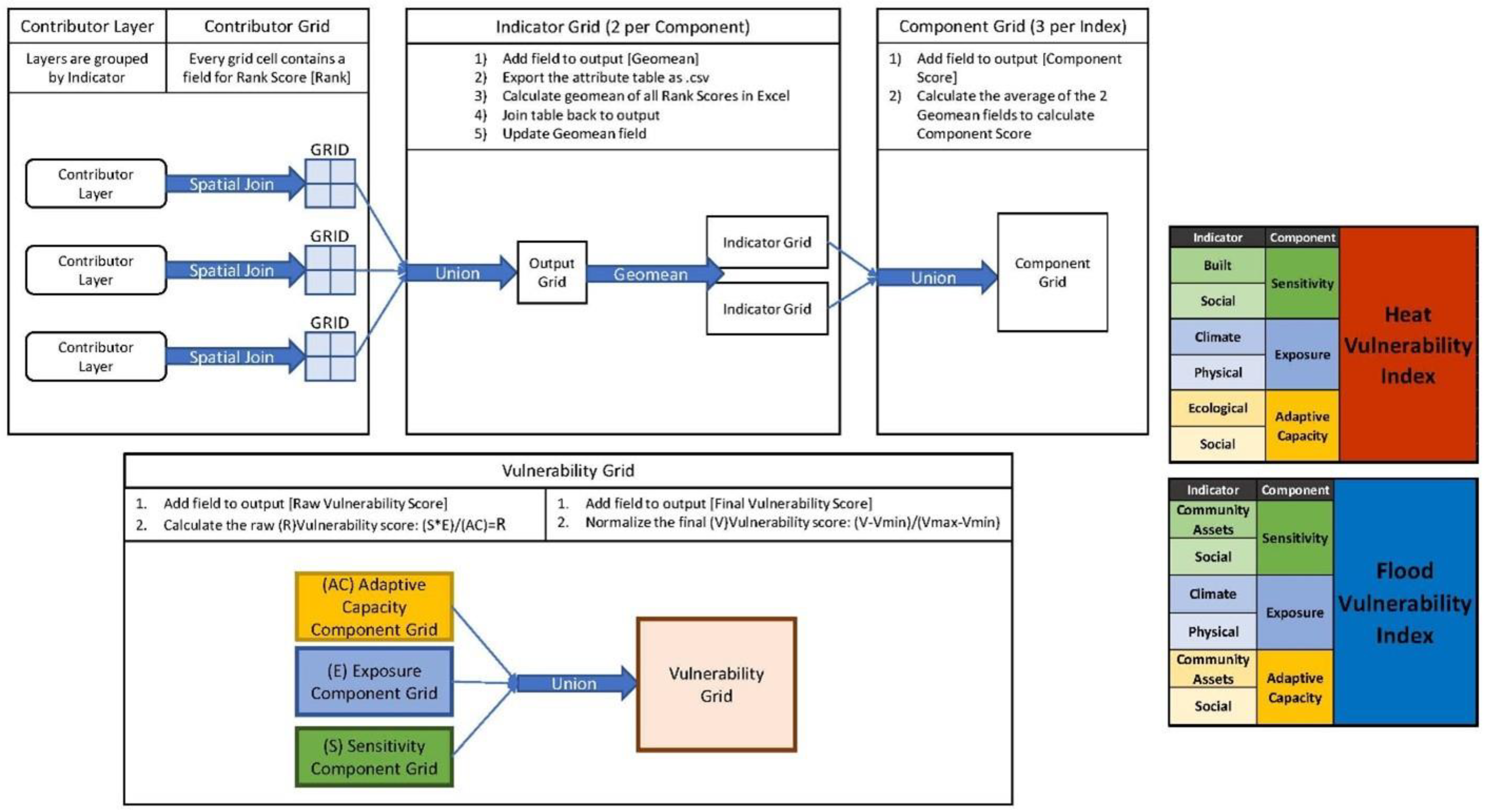
Comprising the exposure, sensitivity, and adaptive capacity framework defined in the IPCC framework [9,10], we identified indicators that reflect Connecticut-specific stressors related to flooding and extreme heat. The indicator selection was based on a search of the literature, available spatially consistent data, and relevance to stakeholder priorities identified through engagement sessions. Contributing spatial information is categorized under social, built, and ecological environments, and then distributed to exposure, sensitivity, and adaptive capacity components (Figure 1). A full list of indicators and their classification under flood and heat vulnerability categories is provided in

Table 1. List of indicators of CCVI 2.0 categorized by their components and their source [19]. The Component Category column refers to the three sub-indices: Exposure, Sensitivity, or Adaptive Capacity. The Indicator Type column refers to the categorized indicators under similar features. The Indicator is the gridded processed data. All the hlinks were accessed on 21 May 2025. The datasets and their ranking are in the Supplemental Materials, Flood and Heat CCVI Data Classification tables.

CCVI	Component Category	Indicator Type	Indicator	Data Source
Flood	Adaptive Capacity	Community Assets	Proximity to Healthcare Facility	Homeland Infrastructure Foundation-Level Data (HIFLD) (https://hifld-geoplatform.hub.arcgis.com/pages/hifld-open), Hospitals & Urgent Care Facilities
			Proximity to Shelter	COG provided data supplemented with CT DEMHS (https://portal.ct.gov/despp/services/emergency-management-and-homeland-security?language=en_US) and municipal websites
			Proximity to Major Roadways	CT DOT Roadway Classifications and Exits (https://connecticut-ctdot.opendata.arcgis.com/maps/65d7254355bb4466871cd7c5ea8a6a5d/about)
			Public Water Service Area	CT Water Supply Plan (DPH) (https://maps.ct.gov/portal/apps/experiencebuilder/experience/?id=1a8bf90b37b24affaeb41a41d71c9417&draft=true)
			Regulatory Standards	Municipal Websites, provided by CIRCA
			Sewer Service Areas	CT DEEP (https://maps.ct.gov/portal/apps/experiencebuilder/experience/?id=1a8bf90b37b24affaeb41a41d71c9417&draft=true)
			Percent Open Space in SFHA	CT DEEP (2022) (https://geodata.ct.gov/datasets/CTDEEP::protected-open-space-view/about)
			Resilient Landscapes	The Nature Conservancy (https://www.conservationgateway.org/ConservationByGeography/NorthAmerica/UnitedStates/edc/reportsdata/terrestrial/resilience/Pages/default.aspx)
			Water Company Land	CT DPH (https://maps.ct.gov/portal/apps/experiencebuilder/experience/?data_id=dataSource_1-Exclusive_Service_Areas_1710%3A%2CdataSource_1-Private_Well_Parcels_4899%3A%2CdataSource_1-Connected_Sewer_Service_Areas_8716%3A%2CdataSource_1-ESA_Changes_6777%3A%2CdataSource_1-Drinking_Water_Watersheds_5159%3A199%2CdataSource_1-Aquifer_Protection_Areas_312%3A%2CdataSource_1-Connecticut_CAMA_and_Parcel_Layer_6551%3A%2CdataSource_1-SourceWater_1012%3A%2CdataSource_1-Buffered_Community_PWS_Service_Areas_3916%3A&draft=true&id=1a8bf90b37b24affaeb41a41d71c9417)
		Social	Percent of Owner-Occupied Housing Units	DP04: Census ACS 2015–2019 5-year Estimates (https://www.census.gov/programs-surveys/acs/technical-documentation/table-and-geography-changes/2019/5-year.html)
			2022 Average Disposable Income (Esri)	ESRI (https://www.arcgis.com/home/item.html?id=706993115a5842f6b45d563d35a74109), U.S. Census Bureau
			Percent Housing Units with No Vehicle Present	DP04: Census ACS 2015–2019 5-year Estimates (https://www.census.gov/programs-surveys/acs/technical-documentation/table-and-geography-changes/2019/5-year.html)
	Exposure	Climate	CIRCA-Modified Flood Zone (Q3, DFIRM, Preliminary)	FEMA (https://www.fema.gov/flood-maps)
			CIRCA Sea Level Rise	CIRCA-Mean High High Water with 20-inch sea level rise (https://resilientconnecticut.uconn.edu/datasets/connecticut-sea-level-rise-viewer/)
			Storm Surge	SLOSH Category 4 data from NOAA (https://www.arcgis.com/home/item.html?id=1b2c267aa3a547ba9eea5e40faa3b9c2)
		Physical	Elevation Pooling	CT ECO 2016 LIDAR (https://maps.cteco.uconn.edu/data/flight2016/)
			Erosion Susceptibility	CT DEEP (https://ct-deep-gis-open-data-website-ctdeep.hub.arcgis.com/datasets/erosion-susceptibility/explore)
			Shoreline Change Rate	NOAA, NGS, CT DEEP
			Impervious Surfaces	CT ECO 2012 Impervious Surface (https://maps.cteco.uconn.edu/projects/ms4/impervious2012/)
			Soil Drainage	SSURGO Soil Drainage Class (https://www.nrcs.usda.gov/resources/data-and-reports/soil-survey-geographic-database-ssurgo)
	Sensitivity	Community Assets	Brownfields	CT DEEP (https://portal.ct.gov/deep/remediation--site-clean-up/brownfields/brownfields-site-inventory)
			Proximity to Bus Hubs (Plus transit, bus stations)	US DOT Bureau of Transportation Statistics (https://www.bts.gov/), SLR
			Critical Facilities	Compiled from Natural Hazard Mitigation Plans, COG-provided data, and CT DEMHS
			Railroad Stations	CT Open Data for railroads—joined to building footprints. (https://geodata.ct.gov/datasets/CTDEEP::connecticut-railroads/explore?location=41.517557%2C-72.747450%2C7.69)
			Roadways	CT DOT (https://connecticut-ctdot.opendata.arcgis.com/maps/5e334f57a37f4eaa970b0ee5a52624d0/about)
			Railways	CT DEEP (https://ct-deep-gis-open-data-website-ctdeep.hub.arcgis.com/datasets/connecticut-railroads/explore)
			Septic Areas (outside of sewer service area)	SLR erased the CT DEEP sewer service area from the project boundary (https://ct-deep-gis-open-data-website-ctdeep.hub.arcgis.com/datasets/CTDEEP::connected-sewer-service-areas/explore)
			Private Wells in SFHA	CT DWVARP (https://portal.ct.gov/dph/drinking-water/dws/drinking-water-vulnerability-assessment-and-resilience-plan-dwvar-plan)
			Building Density	CT ECO 2012 Impervious Surface (https://maps.cteco.uconn.edu/projects/ms4/impervious2012/)
			Historic Buildings (SHPO)	SHPO (https://portal.ct.gov/DECD/Content/Historic-Preservation), Dewberry
			Critical Habitat	CT DEEP (https://ct-deep-gis-open-data-website-ctdeep.hub.arcgis.com/datasets/critical-habitats/explore)
			Public Water Supply Watersheds	CT DPH watersheds (WUCC/DPH) (https://maps.ct.gov/portal/apps/experiencebuilder/experience/?id=1a8bf90b37b24affaeb41a41d71c9417&draft=true)
		Social	Household Median Income	S1901_C01_012E	Census ACS 2015–2019 5-year Estimates (https://www.census.gov/programs-surveys/acs/technical-documentation/table-and-geography-changes/2019/5-year.html)
			Over 5 with a Disability	B18101
			Percent Living Below 185% Federal Poverty Level	S1701_C01_041E
			Percent Over 25 without a high school diploma	S0601_C01_033E
			Percent Over 65	S0101_C02_030E
			Percent population under 5	S0101_C02_002E
			Percent population unemployed	DP03_0005PE
			Population density	S0101
			Non White Population	S0601_C01_022E
			Speaks English less than well/not at all	S0601_S0601_C01_026E
			Over 65 Living Alone (households)	B25011
			Single-parent households	DP02
Heat	Adaptive Capacity	Ecological	Percent Tree Cover	USFS 2016 Percent Tree Canopy (https://data.fs.usda.gov/geodata/rastergateway/treecanopycover/)
			Normalized Difference Vegetation Index (NDVI)	CIRCA provided Landsat 8 image processed through median values from 2013–2022 during all summers (June–September), see Supplementary Material
		Social	Proximity to Bus Hubs (Plus transit, bus stations)	US DOT Bureau of Transportation Statistics (https://www.bts.gov/), CT DOT
			Percent population with (no) health insurance	B27010 Census ACS 2015–2019 5-year Estimates
			Proximity to Swimming Areas	CIRCA and SLR compiled swimming area data from CT DEEP (https://portal.ct.gov/deep/state-parks/recreation-information/swimming---ct-state-parks-and-forests) and CT DPH (https://portal.ct.gov/dph/environmental-health/recreation/public-pools)
			Proximity to Healthcare Facility	Homeland Infrastructure Foundation-Level Data (HIFLD) (https://hifld-geoplatform.hub.arcgis.com/pages/hifld-open), Hospitals & Urgent Care Facilities
			Proximity to Shelter	COG provided data supplemented with CT DEMHS (https://portal.ct.gov/despp/services/emergency-management-and-homeland-security?language=en_US) and municipal websites
			Proximity to Cooling Center	CIRCA provided known cooling center locations based on consultations with municipalities in 2022.
	Exposure	Climate	Maximum Land Surface Temperature	CIRCA provided Landsat 8 image processed through median values from 2013–2022 during all summers (June–September), see Supplementary Material
		Physical	Emissivity	CIRCA provided Landsat 8 image processed through median values from 2013–2022 during all summers (June–September), see Supplementary Material
			Roadway Usage Classification (Traffic Emissions)	CT DOT (https://geodata.ct.gov/maps/65d7254355bb4466871cd7c5ea8a6a5d/about)
			Impervious surfaces	CT ECO 2012 Impervious Surface (https://maps.cteco.uconn.edu/projects/ms4/impervious2012/)
	Sensitivity	Built	Private Well Coverage	CT DWVARP (https://portal.ct.gov/dph/drinking-water/dws/drinking-water-vulnerability-assessment-and-resilience-plan-dwvar-plan)
			Median Structure Age	B25035_001E: Census ACS 2015–2019 5-year Estimates (https://www.census.gov/programs-surveys/acs/technical-documentation/table-and-geography-changes/2019/5-year.html)
			Public Housing Units	US Dept of Housing and Urban Development (https://www.huduser.gov/portal/pdrdatas_landing.html) & B25001 Census ACS 2015–2019 5-year Estimates (https://www.census.gov/programs-surveys/acs/technical-documentation/table-and-geography-changes/2019/5-year.html)
		Social	Average number of emergency visits for asthma, per 10,000 population	CT DPH Asthma Statistics, 2012–2019 age-adjusted rate of emergency department visits per 10,000 (https://portal.ct.gov/DPH/Health-Education-Management--Surveillance/Asthma/Asthma-Statistics)
			Heat Stress	CT DPH 2013–2017 heat stress-related emergency department visits per 100,000 (https://maps.ct.gov/portal/home/item.html?id=ac51c59d5f6d4295afb940c363217bf8)
			Percent living below 185% of the federal poverty level	S1701_C01_041E	Census ACS 2015–2019 5-year Estimates (https://www.census.gov/programs-surveys/acs/technical-documentation/table-and-geography-changes/2019/5-year.html)
			Percent over 25 without a high school diploma	S0601_C01_033E
			Population density	S0101
			Outside Employment	US Census OnTheMap (https://onthemap.ces.census.gov/)

.

The CCVI 1.0 coverage area consisted only of Fairfield County and New Haven County. For the CCVI 2.0, coverage was expanded to the entire state of Connecticut. We also made some adjustments to the indicator categories and factor list between the 1.0 and 2.0 versions, such as including additional factors identified by the project team as contributing to overall vulnerability (i.e., a factor for roadway usage classifications to the heat exposure component score) or removing factors that lacked a robust connection to vulnerability (i.e., a factor for a statewide Natural Diversity Data Base). A full list of indicators for the 1.0 and 2.0 versions of the CCVI can be found in Supplemental Materials, Table: Changes of the indicators from CCVI 1.0 to 2.0.

2.2. Data Processing and Workflow

The CCVI integrates diverse datasets into a consistent, interpretable vulnerability score. The index was constructed using a multi-step geospatial analysis. The index was designed to combine exposure, sensitivity, and adaptive capacity scores by assigning rankings to dozens of geospatial layers in ArcGIS Pro. These layers were systematically organized within ArcGIS Enterprise geodatabases to mirror the methodological sequence of data processing steps, as outlined in Table 1.

The process starts with generating a standardized spatial grid (with 200 × 200 m grid cells), which serves as the foundation for joining and analyzing all contributing datasets. This source grid excluded cells primarily covered by water, defined as over 70% water coverage for heat analysis and 85% for flood analysis, using the USGS National Hydrography Dataset. Before beginning the data analysis stage, data management and organization are done by collecting all the “Contributing Layers” (raw GIS data, i.e., Building Footprint) and preparing geodatabases to store both the contributing layers and the indicator grids. Each dataset used as an indicator was prepared for analysis by formatting key fields, removing extraneous attributes, and creating placeholder fields for rank scores. These datasets were spatially joined (based on overlapping spatial relationships) to the source grid using appropriate statistical methods (e.g., average, maximum) to assign representative values to each grid cell. The outcome of this joint was a “Contributor Grid,” which contained both raw values and rank scores for each variable (Figure 2).

Next, contributor grids were grouped and aggregated into “Indicator Grids”, reflecting broader vulnerability categories such as Social, Ecological, Physical, Climate, and Community Assets. Within each indicator, the rank scores (0 indicates no or not available data and ranks ranging from 1, least impacted, to 5, most impacted) of contributing layers were combined using the geometric mean. For example, the heat physical exposure indicator for impervious surfaces was ranked by the percentage area of each grid cell covered by impervious surfaces, with higher impervious surface coverage receiving higher exposure rankings (i.e., an area with 0–5.5% impervious surface is ranked 1, while an area with 53.2–100% is ranked 5). On the other hand, the heat social adaptive capacity indicator for percent population with no health insurance follows an inverse ranking, as lower percent population with no health insurance received higher adaptive capacity rankings (i.e., 17.3 –34.4% is ranked 1, while 0–2.7% is ranked 5). For more details on individual indicator rankings, refer to the data classification Flood and Heat CCVI Classification tables in the Supplemental Materials.

To rank each indicator, the attribute table of each indicator grid was exported as a .csv file, fields were cleaned to include only rank values and grid IDs, and the geometric mean was calculated after removing zero values. This value was rejoined to the indicator grid and stored in a new field labeled “Geomean,” representing the vulnerability score at the indicator level (Figure 3). Indicator Grids were then aggregated into Component Grids, corresponding to the three components of vulnerability: Exposure, Sensitivity, and Adaptive Capacity. A union of the relevant indicator grids was performed, and a new field called “Component Score” was created. The average of the Geomean scores for each indicator within the component was used to calculate the Component Score for each cell.

The final vulnerability score was derived by integrating the three component scores using

$$Vulnerability={\displaystyle \frac{Exposure\times Sensitivity}{AdaptiveCapacity}},$$

(1)

This calculation produced the vulnerability score for each grid cell. To ensure consistency and comparability across space, these raw values were then normalized using.

$$NormalizedVulnerability={\displaystyle \frac{\left(V-V_{min}\right)}{\left(V_{max}-V_{min}\right)}},$$

(2)

where V is the vulnerability score, $V_{min}$ is the minimum vulnerability score, and $V_{max}$is the maximum vulnerability score in the series. The resulting final normalized vulnerability score ranges between 0 and 1, where 0 represents the least vulnerable areas and 1 the most vulnerable. This score served as the basis for the Flood and Heat Vulnerability Indices.

2.3. Stakeholder Feedback

The feedback process from the stakeholders was embedded through in-person workshops, online collaborative sessions, surveys, and municipal meetings. During breakout sessions of the CIRCA Annual Summit in 2019, we presented early findings from version 1.0 and solicited real-time feedback on which contributing information the stakeholders have an interest in. Another engagement effort occurred through the Resilient Connecticut Collaborative in 2020, a working group of municipal officials, transportation and utility agencies, and non-profit organizations. A targeted feedback session was held with this group, focused on usability and implementation. Participants emphasized the need for clearer data visualization, broader geographic coverage, and more specific, community-relevant indicators. Additional feedback was gathered through a presentation at a meeting of Connecticut’s interagency resilience working group, State Agencies Fostering Resilience (SAFR). This includes representatives from the Department of Transportation, Public Health, Housing, Emergency Management, Homeland Security, and Energy and Environmental Protection. We also held two regional workshops in 2021 to elicit feedback from four Councils of Governments (COGs) with responsibilities in New Haven and Fairfield Counties. These sessions provided an opportunity to present the evolving CCVI framework to a group with a unique understanding of interagency planning challenges.

Stakeholder engagement efforts were expanded with the development of CCVI 2.0. From 2022–2023, the CIRCA team presented CCVI 2.0 maps at local town planning meetings across central and southeastern Connecticut and CCVI results were incorporated into hazard discussions during the development of two regional hazard mitigation plans. The CCVI 2.0 engagement allowed municipal staff to comment on the tool directly to CIRCA staff rather than pass their input through the COGs. Additionally, we gathered feedback through webinar sessions and a survey embedded in the CCVI webpage on CIRCA’s website.

2.4. Principal Component Analysis (PCA)

We also performed principal component analysis (PCA) for exposure, sensitivity, and adaptive capacity. There are two goals of this analysis: (i) to assess whether certain indicators were conveying overlapping information, and (ii) to understand which combinations of indicators (principal components) explained the most spatial variation in vulnerability across Connecticut. This analysis helped reveal the dominant patterns of the indicators for each component. The results of this analysis are aimed at improving the indicator selection and weighting of the future iterations of CCVI.

2.5. Online Mapping Application

The accessibility of the CCVI, a large dataset containing approximately 350,000 grid cells and numerous attributes, is essential to support planners and state agencies in climate resilience and hazard mitigation planning. However, the file’s size and complexity posed technical challenges when uploading to ArcGIS Online, making it difficult to host as a standard feature layer. To improve performance and visualization in web maps, the data was converted into vector tiles, a format that breaks geographic data into small, pre-rendered tiles optimized for display. While vector tiles retain feature geometry and styling, they do not preserve the underlying attribute data needed for analysis and integration into planning workflows. To ensure that users could still access the complete vulnerability dataset, the original feature layer was included beneath the vector tile layer. In ArcGIS Experience Builder, the application was configured so that the vector tiles are visible from the global to metropolitan scale, while the full feature layer with identical symbology becomes active at finer zoom levels (metropolitan area to room). This enabled a full statewide visualization of heat and flood vulnerability while also maintaining access to the detailed data at a finer scale. The Heat CCVI is available via the following link: Heat CCVI Experience Builder (https://experience.arcgis.com/experience/a364a5f4870c4dc7ba53c681543521af/ accessed on 21 May 2025). Similarly, the Flood CCVI is available via the following link: Flood CCVI Experience Builder (https://experience.arcgis.com/experience/44ddea38aac34779a6a115ed6eae1db1/ accessed on 21 May 2025). To download and access the underlying datasets for each index, navigate to the “Data and Statistics” tab within the respective applications. All the documentation of the CCVI can be accessed from the website given in the Supplementary Materials.

3. Results

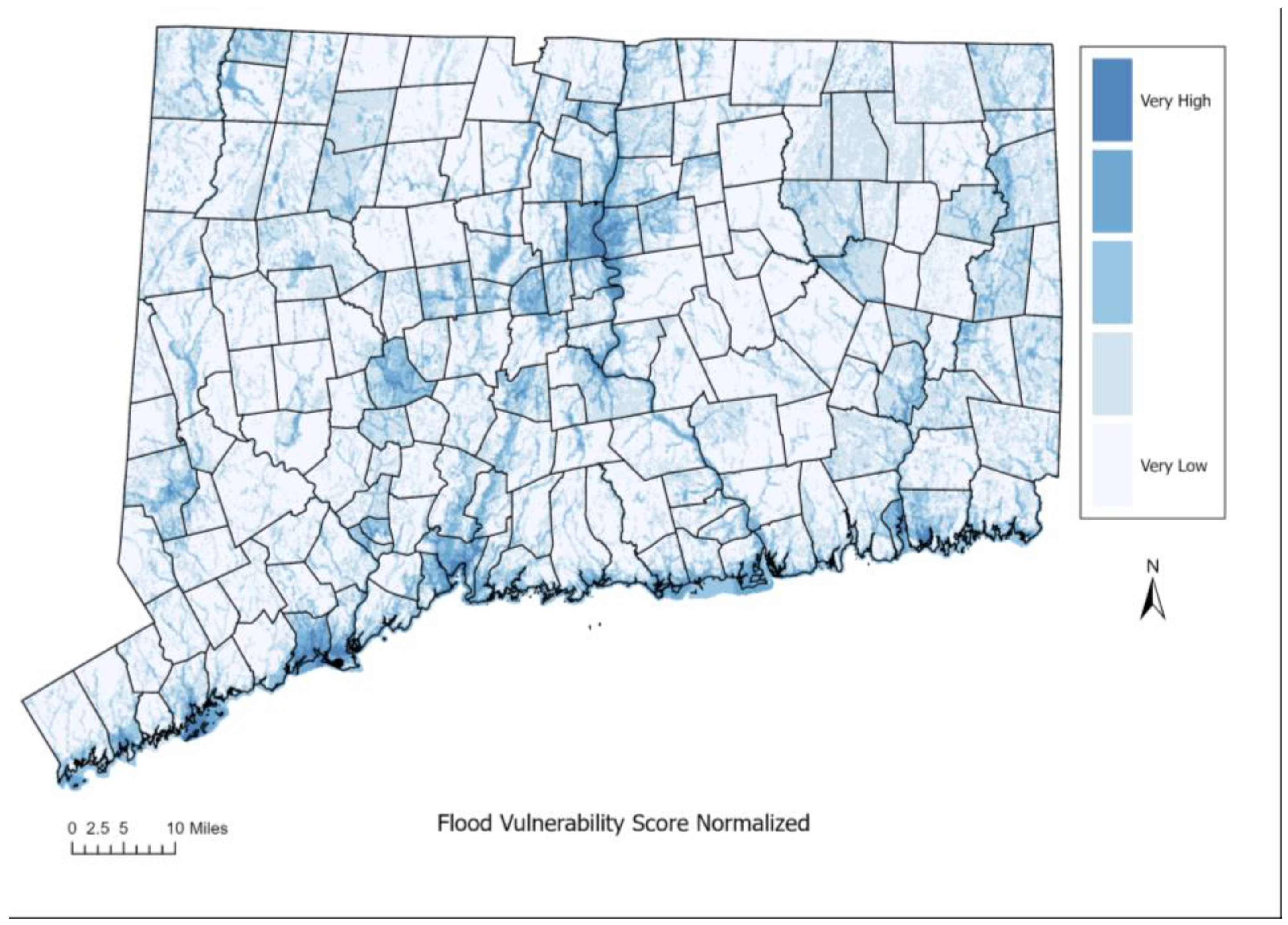
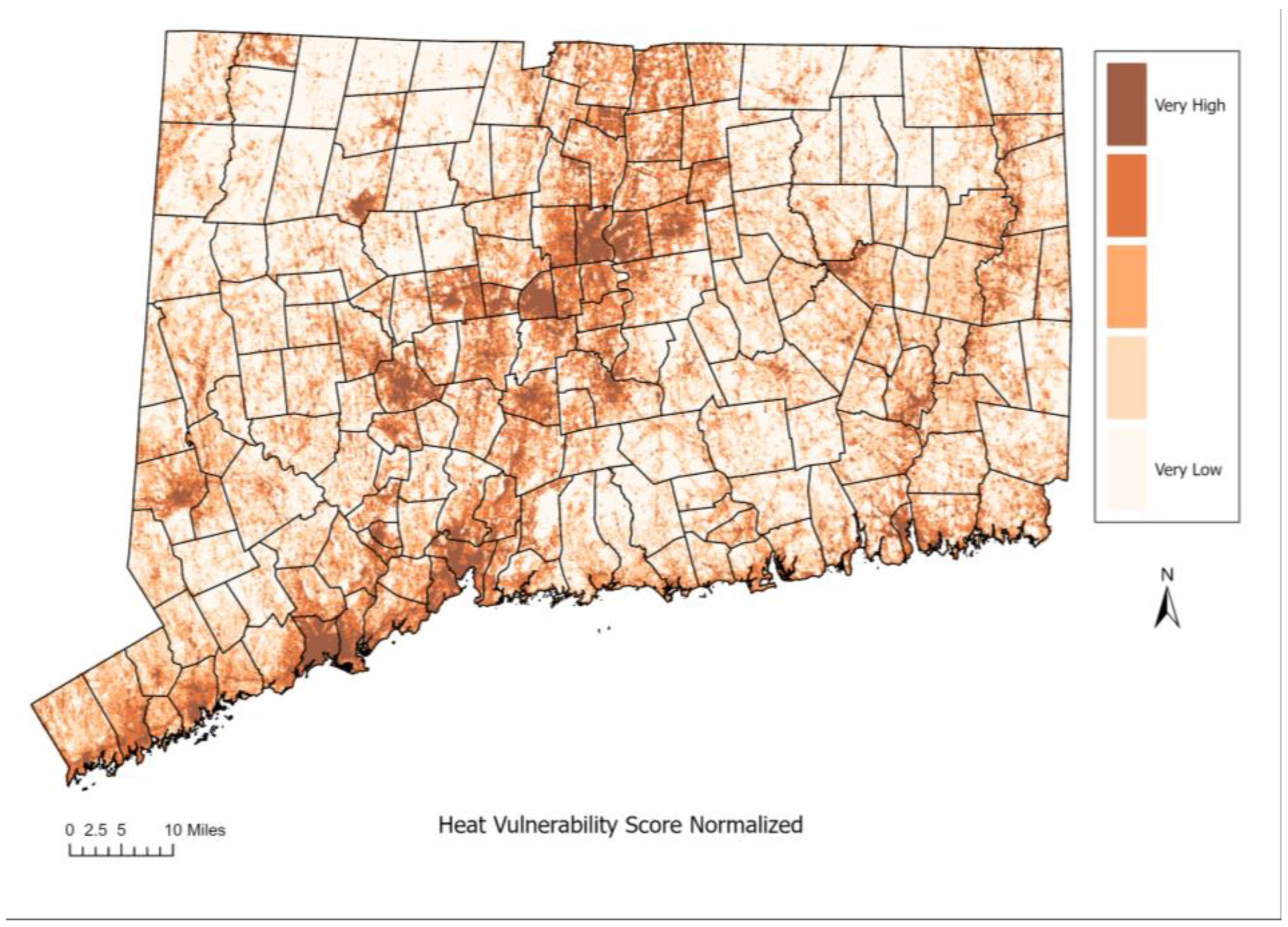
The statewide maps (Figure 4 and Figure 5) demonstrate the wide range of vulnerability experienced within Connecticut for both flood and extreme heat, indicating that approaches to mitigating this vulnerability should be regionally and locally tailored for the greatest effect. Statewide view of normalized flood vulnerability scores, displayed with a five-class natural breaks (Jenks [21]) classification system. The statewide view of the normalized flood and heat vulnerability scores gives distinct patterns (Figure 4 and Figure 5), which requires an in-depth analysis of the regional variations and the underlying dominant indicators causing Connecticut’s vulnerability. The following sections of the results will focus on the patterns of rural vs. non-rural, coastal vs. inland, heat vs. flood vulnerability distribution, as well as Principal Component Analysis (PCA) results revealing the dominating indicators contributing to these vulnerabilities.

3.1. Rural vs. Non-Rural Vulnerability

We classified Connecticut towns as rural or non-rural based on the designations provided by the Connecticut Office of Rural Health (CT-ORH). According to CT-ORH, a town is considered rural if it meets two criteria: a total population of 10,000 residents or fewer, and a population density of less than 500 people per square mile. This definition was established to guide strategic planning and determine eligibility for financial support from CT-ORH. We used this definition to inform our designation of “rural” and “non-rural” municipalities for our analysis, as Connecticut does not otherwise have standardized accepted definitions for suburban or urban communities.

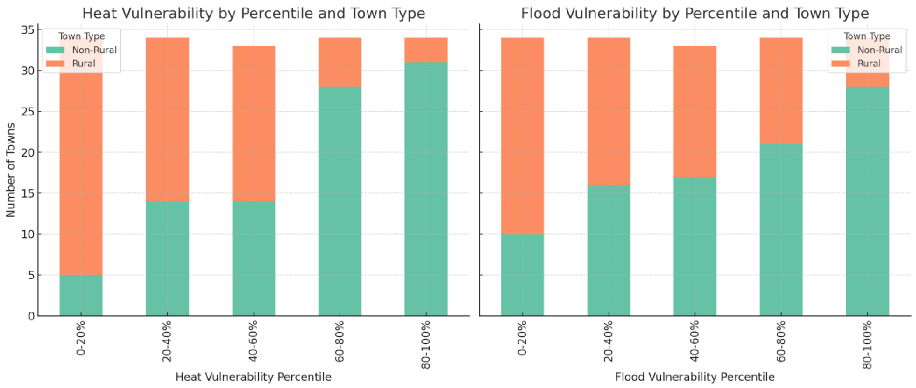
Analysis of town-level data in Connecticut reveals a relationship between rural and non-rural towns, and vulnerability to flooding and extreme heat. In Figure 6, in the case of heat vulnerability (left panel), a trend emerges with towns with higher heat vulnerability percentiles more likely to be non-rural. In the lowest vulnerability bracket (0–20%), the majority of towns are rural, while in the highest vulnerability bracket (80–100%), the majority of towns are non-rural. This suggests that non-rural areas in Connecticut face a disproportionately higher burden of heat-related vulnerability compared to rural areas, which is consistent with expectations since rural towns tend to have indicator values associated with lower vulnerability, such as higher tree cover and lower impervious surfaces. For flood vulnerability (right panel in Figure 6), a similar but less pronounced trend is observed. While rural towns are more prevalent in the lower percentiles (0–40%), non-rural towns become more dominant as vulnerability increases, especially in the 60–100% range. However, the distribution remains more mixed than with heat vulnerability, indicating that both rural and non-rural towns are significantly affected by flood vulnerability, though higher vulnerability still skews toward non-rural areas.

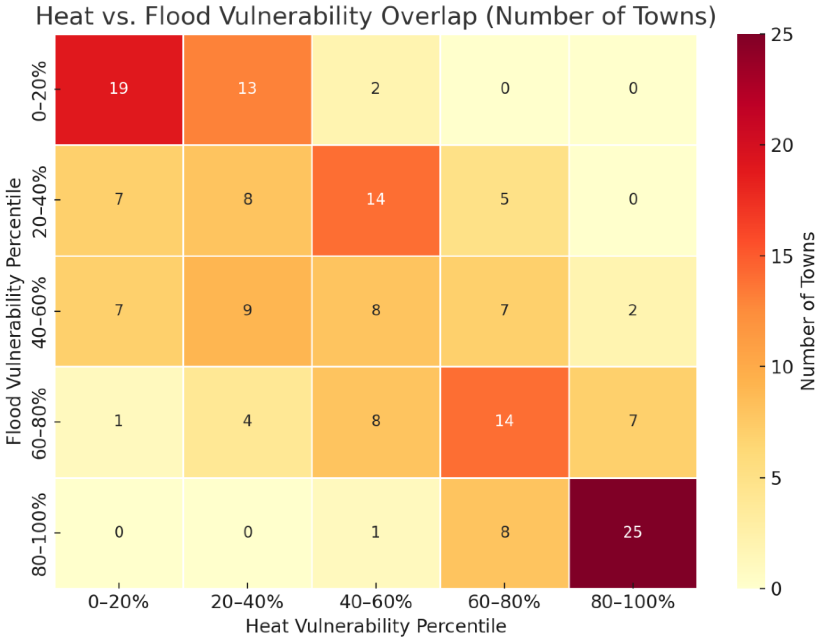
Figure 7 highlights the distribution of Connecticut towns across heat and flood vulnerability across the percentiles. Figure 7 shows that there is a clear spatial clustering of vulnerability. The categorization of rural and non-rural towns used in Figure 7 is given in the Supplementary Materials, Rural and Non-Rural Town Ratio by Percentile Bins table. The 80–100 Percentile bin for both flood and heat vulnerability contains 25 towns, of which 22 are classified as non-rural. This overlapped high-vulnerability cluster includes major cities such as Bridgeport, the largest city in Connecticut by population, Hartford, New Haven, Waterbury, and New London. The towns that are highly ranked for both heat and flood vulnerability will require location-specific adaptation options. These urban areas experience compound vulnerability due to their physical exposure, dense built environments, and high social sensitivity. In contrast, the 0–20% vulnerability bin for both heat and flood contains 19 towns, 15 of which are rural. Bethlehem, Colebrook, Franklin, Salem, and Woodstock, among many others, show lower exposure and higher adaptive capacity due to greater green space coverage, lower impervious surface area, and fewer socially sensitive populations. Rural towns with lower population densities, including Hartland, Barkhamsted, Eastford, and Colebrook, have the lowest average heat vulnerability. The lowest average flood vulnerability is seen in a mix of rural and non-rural towns, including Tolland, Granby, and Weston (non-rural), and Colebrook and Hebron (rural). Notably, the distribution reveals a diagonal ridge from the top-left to the bottom-right of the matrix, indicating considerable co-vulnerability—towns vulnerable to flooding also seem to be vulnerable to heat, while others have low vulnerability to both. Mid-range overlap is also apparent, with several towns concentrated in central combinations—for instance, 14 towns in both the 20–40% flood and 40–60% heat vulnerability ranges, and another 14 in the 60–80% range for both hazards. The 40–60 and 60–80 percentile bins represent a more balanced distribution of rural/non-rural town types with moderate levels of vulnerability. For Connecticut, rural towns are distributed across the full vulnerability spectrum.

3.2. Coastal vs. Inland Vulnerability

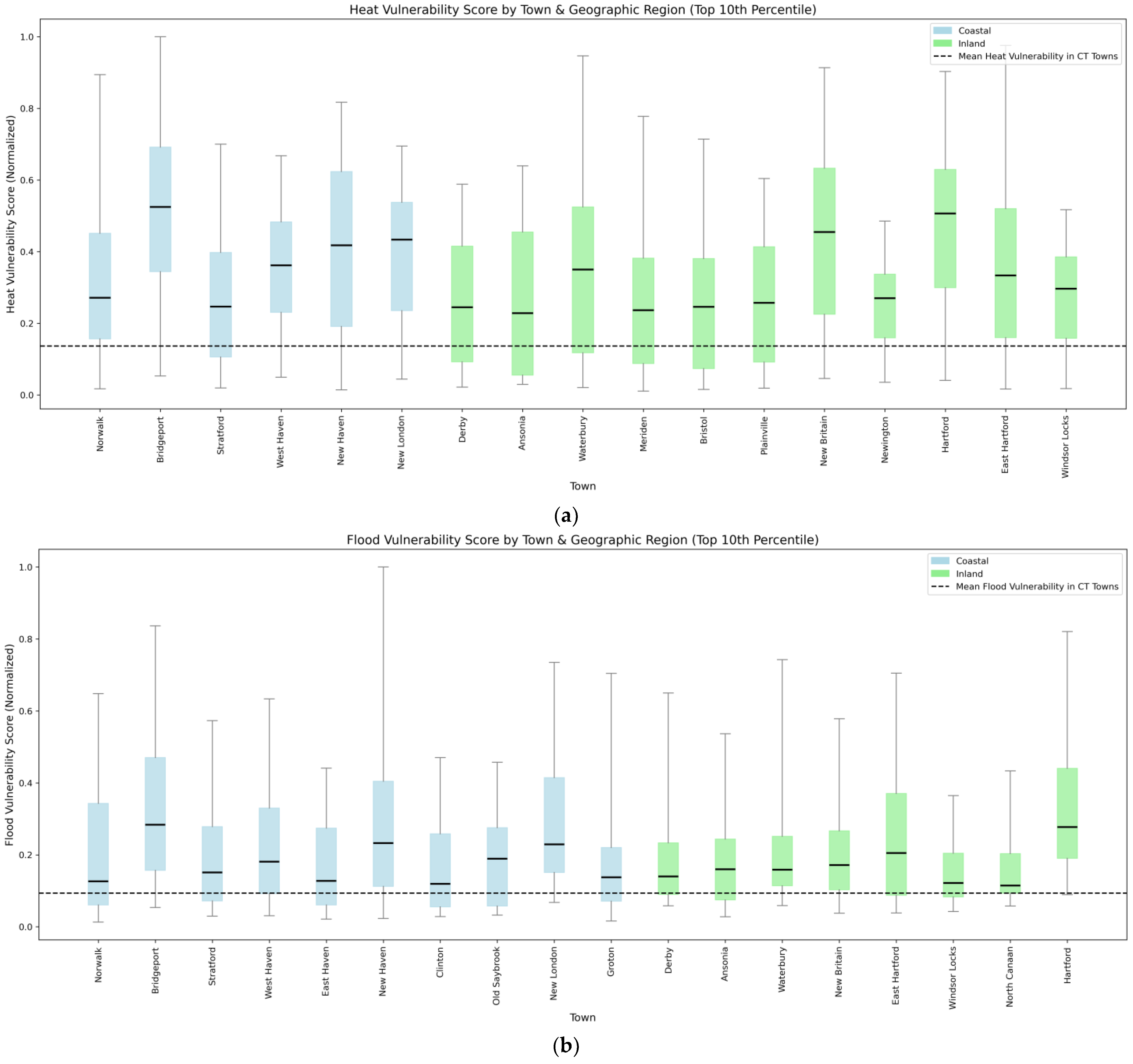
Flood and heat vulnerability scores were assessed across Connecticut towns and grouped by geographic region (coastal vs. inland) for those in the top 10th percentile of vulnerability (Figure 8).

Flood vulnerability was more prominent in coastal municipalities. Of the 18 towns in the top 10th percentile for normalized flood vulnerability scores, 10 (56%) were coastal and 8 (44%) were inland. Several coastal towns—such as Bridgeport, New Haven, and New London—had median flood vulnerability scores well above the overall 169 town (all towns) mean (indicated by the dashed line). However, certain inland towns like Hartford and East Hartford also exceeded the all-town mean, suggesting that flood risk is not limited to the coast in Connecticut and inland municipalities are susceptible to riverine flooding.

In contrast, heat vulnerability was more concentrated in inland towns. Of the 17 towns in the top 10th percentile, 11 (65%) were inland and 6 (35%) were coastal. Inland towns such as Hartford, East Hartford, and Bristol had notably high median heat vulnerability scores above the all-town mean. Coastal towns like Bridgeport and New Haven also ranked high for heat exposure, though the inland dominance suggests that factors like low tree canopy and extensive impervious surfaces drive greater heat risk in non-coastal areas.

3.3. Heat vs. Flood Vulnerability

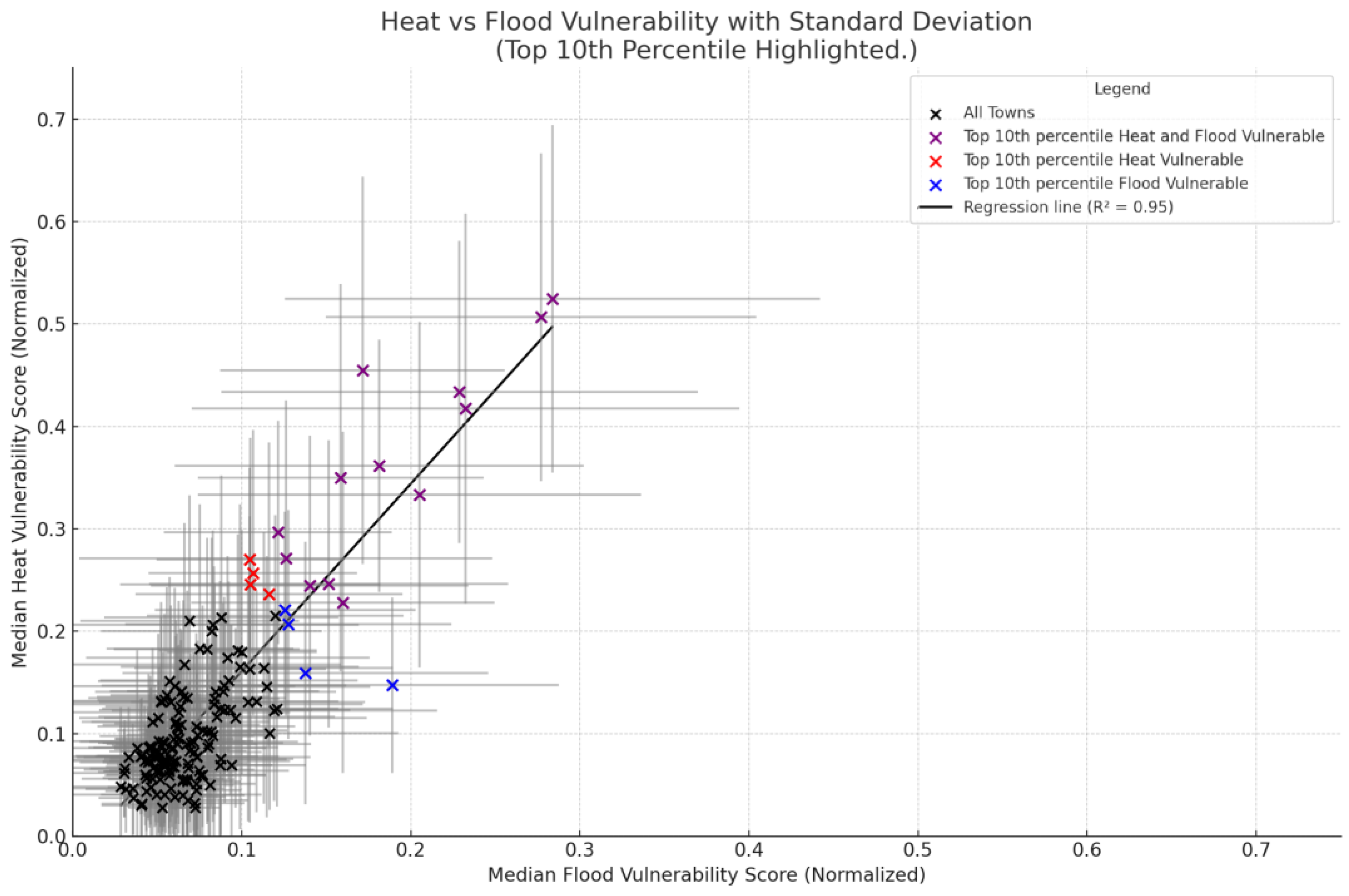
Figure 9 displays the median heat and vulnerability scores for all 169 Connecticut municipalities with standard deviation crossbars. The standard deviation represents the distribution of the index within the town boundary. Of the 90th percentile, 12 towns (7.1%) were classified as being highly vulnerable to both heat and flooding (purple symbols), indicating that they have a compound climate vulnerability. These towns include Bridgeport, Hartford, New London, New Haven, East Hartford, West Haven, New Britain, Norwalk, Waterbury, Stratford, Windsor Locks, Ansonia, and Derby. These municipalities not only face structural exposure (e.g., impervious surfaces, poor drainage, or aging infrastructure) but also tend to have high social sensitivity indicators, such as income vulnerability, elderly populations, and limited access to cooling or evacuation resources. An additional 4 towns (2.0%) in the top 10th percentile, including Plainville, Newington, Meriden, and Bristol, were identified as highly vulnerable to heat, shown in red. These towns demonstrate elevated urban heat island effects, limited greenspace, and in some cases, insufficient social adaptive capacity, contributing to their top 10% heat vulnerability classification. Another 5 towns (3.0%) are in the top 10th percentile, including Old Saybrook and Groton. East Haven, Clinton and North Canaan were highly vulnerable to flooding, represented by light blue. These towns are around the major floodplains. The remaining 148 towns out of the 169 total towns in CT, 87.5%, did not meet the 90th percentile threshold for either heat or flood vulnerability and are categorized as lower relative risk. This distribution highlights the relatively small number of towns facing the highest levels of vulnerability, with a particularly urgent focus needed on the 12 towns experiencing dual exposure. The coefficient of determination (R²) for the regression line fitted to the scatter plot of the median flood and heat normalized vulnerability scores is 0.75. This value suggests a strong positive correlation between the two indices across Connecticut towns, reemphasizing that towns that are more vulnerable to flooding also tend to be more vulnerable to extreme heat. This might be a result of the settlements being made historically along the watershed areas and sharing similar underlying factors in terms of social sensitivity, limited adaptive capacity, and overlapping exposure.

3.4. Underlying Indicators Contributing to Vulnerability

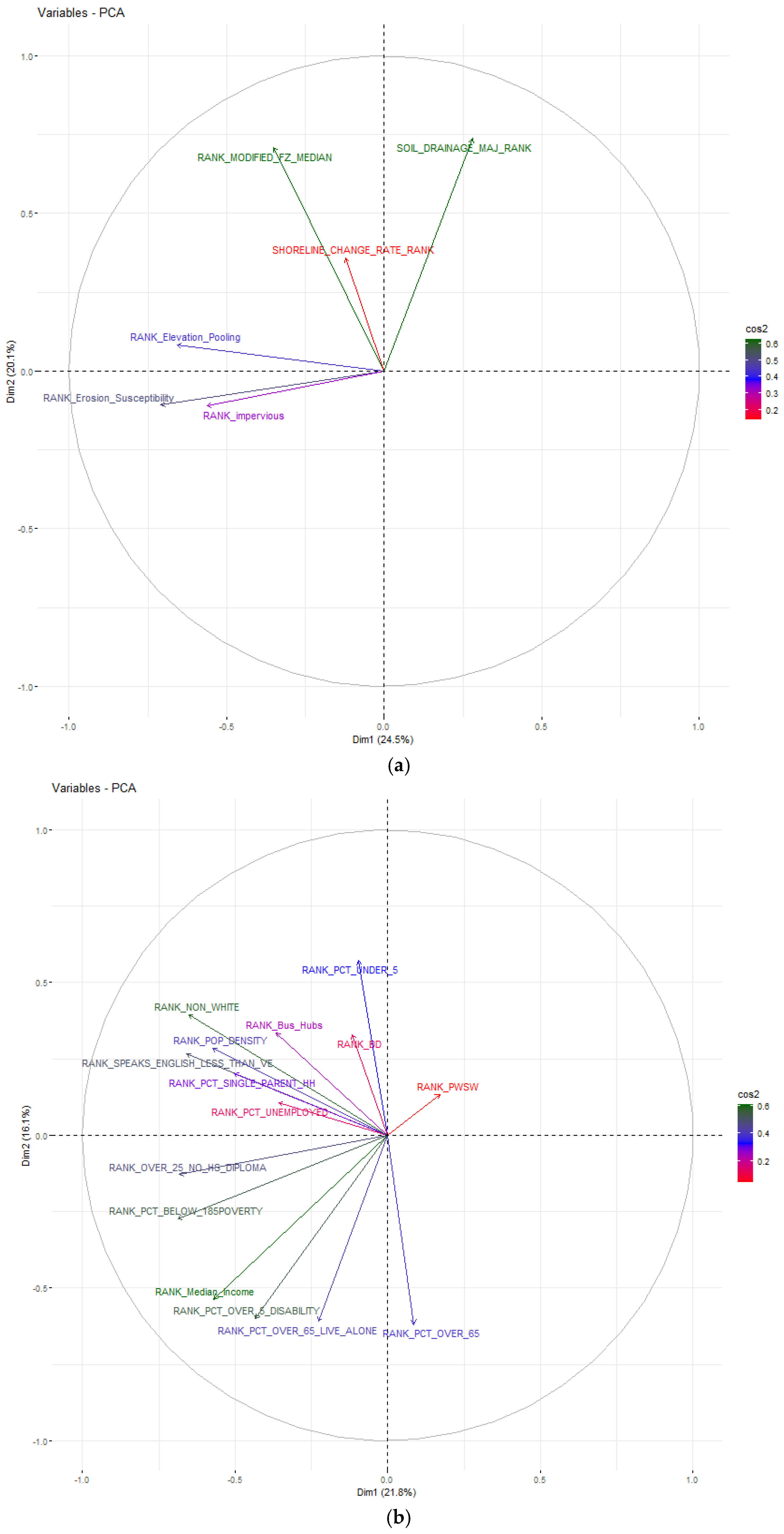
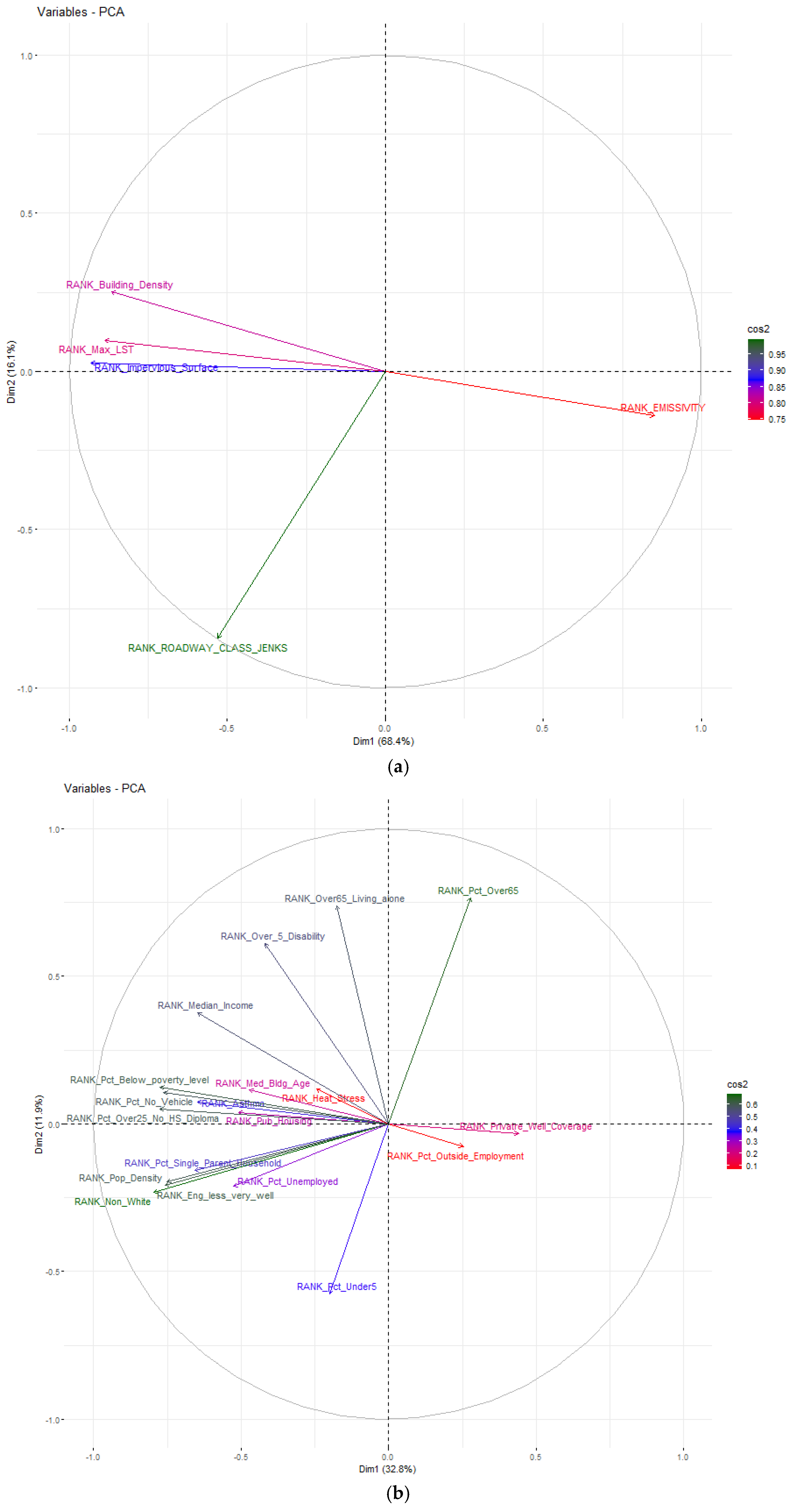
PCA was applied to analyze the internal structure of the Flood and Heat CCVIs, including their subcomponents (Exposure, Sensitivity, and Adaptive Capacity).

Table 2. PCA results of each index, their total variance and dominant PC components.

Index Name	Total Variance (PC1 + PC2)	PC1 Variance (%)	PC2 Variance (%)	PC1 Dominant Indicators	PC2 Dominant Indicators	Highest Cos2 Indicators
Flood CCVI	27.32%	14.86	12.46	% Non-white population, % Speaks English less well, % No vehicle, Public water service area	Median income, Disposable income, % Population with disability, % Owner-occupied housing	Median income, Disposable income, % Below 185% poverty
Flood Exposure	44.62%	24.49	20.13	Erosion susceptibility, Elevation pooling, Impervious surfaces, Modified flood zone median	Soil drainage, Modified flood zone median, Shoreline change rate, Impervious surfaces	Modified Flood Zone Median, Soil Drainage, Erosion Susceptibility
Flood Sensitivity	37.90%	21.76	16.14	% Population below 185% poverty, % Population over 25 with no high school diploma, % Population speaks English less well, % Population non-white	% Population over 65, % Population live alone and over 65, % Population with disability, % Population under 5 years	Median income, % Non-white population, % Population with disability
Flood Adaptive Capacity	52.75%	36.62	16.13	Public Water Service, Regulatory Standards, Proximity to health care facility, major roadways	Disposable income, % Owner-occupied housing, % No access to vehicle, Resilient landscapes	Disposable income, % Owner-occupied housing, % No access to vehicle
Heat CCVI	39.95%	30.15	9.80	Max land surface temperature, Impervious surface, Emissivity, % Population non-white	% Population below poverty level, Median income, % Population over 25 with no high school diploma, Normalized difference vegetation index	% Below poverty level, Normalized difference Vegetation index, Impervious surface
Heat Exposure	84.49%	68.39	16.10	Impervious surface, Max. land surface temperature, Building density, Emissivity	Roadway classifications, Building density, Emissivity, Max land surface temperature	Roadway classification, Building density and impervious surfaces
Heat Sensitivity	44.63%	32.75	11.89	Non-white population, % Below poverty level, % Population over 25 with no high school diploma, % Population with no access to vehicle	% Population over 65, % Population live alone and over 65, % Population with disability, % Population under 5 years	% Population live alone and over 65, % Population with disability
Heat Adaptive Capacity	50.75%	36.78	13.97	Normalized difference Vegetation index, Cooling centers, Proximity to bus hubs, Proximity to healthcare facilities	Swimming area, Swimming access, Swimming proximity, Proximity to bus hubs	Swimming area, Swimming access, Swimming proximity

, Figure 10 and Figure 11 provide a comparative overview, including the total variance explained for the first three principal components, the dominant indicators in the first three principal components (PC1, and PC2), and the highest cos² values, indicating which variables are best represented in PCA. Table 2 illustrates how flood and heat vulnerability are composed of a unique combination of indicators. Additionally, Table 2 shows that the dimensional concentration is not only focused on one PC, indicating that the index design captures the distinct and interrelated domains of vulnerabilities.

In Flood Exposure (Figure 10a), exposure is mostly defined by geophysical conditions and land-use characteristics. PC2 shares similar themes but emphasizes hydrologic patterns. In Flood Sensitivity, PC1 highlights systemic inequity, while PC2 centers on isolation-based sensitivity, and demographic-related issues. These components are conceptually coherent and reinforce the social dimensions of flood sensitivity. In Flood Adaptive capacity, PC1 captures infrastructure and regulatory preparedness; PC2 leans toward financial capacity. Overall, Flood CCVI shows that PC1 focuses on socioeconomic status, and PC2 captures environmental exposure to flooding and infrastructural readiness.

In Heat Exposure (Figure 11) PC1, which relates to the urban heat island effect, is highly dominant and explains the most variance. Future refinement might focus on suburban and vegetative microclimates. PC2 differentiates areas by road density and building patterns. In Heat Sensitivity, similar to Flood Sensitivity, PC1 shows systemic social vulnerability; PC2 captures demographic vulnerability. In Heat Adaptive Capacity, PC1 suggests emphasizing green infrastructure and access to cooling resources, and PC2 is primarily focused on access to water-related recreational infrastructure. Overall, Heat CCVI shows PC1 represents the urban heat island effect compounded by socioeconomic stress, PC2 represents household stability and healthcare access. The index successfully merges exposure and social vulnerability. PCA confirms the dominance of land surface and built environment, indicating the need to strengthen ecological or infrastructure dimensions.

4. Discussion

This section provides the heat and flood vulnerability trends of Connecticut’s 169 towns, and outlines the tool’s strengths and limitations, and its application in adaptation planning.

4.1. Geographic Patterns and Significant Trends of Vulnerability

By synthesizing percentile-based composite scores, disaggregating vulnerability by rural/urban and coastal/inland typologies, and applying principal component analysis (PCA), the results yield actionable insights into localized climate risk and resilience planning.

The findings reinforce that Connecticut’s more densely populated, urban municipalities bear the highest climate vulnerabilities, particularly in terms of dual exposure to both extreme heat and flooding. Urban heat vulnerability appears driven by well-established mechanisms, including the urban heat island effect, impervious surface coverage, and limited greenspace, all of which amplify temperature extremes. Flood vulnerability in these areas is similarly exacerbated by stormwater runoff, aging drainage infrastructure, and proximity to tidal or riverine flood zones.

The majority of towns in the highest vulnerability categories are urban, while rural towns are predominantly clustered in the lower percentiles. This suggests that lower development intensity, tree canopy cover, and ecological buffers in rural areas provide some degree of protection—though exceptions exist, especially in riverine or wetland-dominated rural towns where flood risk persists due to drainage limitations or watershed dynamics.

Geographic differences also reveal important nuances. Coastal towns—such as Bridgeport, New London, and Old Saybrook—register high flood vulnerability consistent with storm surge and sea-level rise exposure. However, inland cities like Hartford, New Britain, and Waterbury emerge as hotspots of heat vulnerability, due to their urban land cover, concentrated populations, and socioeconomic sensitivity.

Even within similar regions, vulnerability varies dramatically from town to town, underscoring the need for localized assessments. For example, Ansonia, Derby, and Naugatuck are geographically small inland towns that register unexpectedly high heat vulnerability, despite their size, due to factors like older housing stock, limited greenspace, and concentrated social sensitivity. North Canaan and East Hartford, though inland, show notably high flood vulnerability, likely driven by riverine flooding, flash flood potential, and limited stormwater capacity. These case studies emphasize that exposure alone does not determine vulnerability. Some towns with high climate exposure exhibit lower overall vulnerability due to strong adaptive capacity, including access to emergency services, municipal investment, or high community capital. Conversely, social sensitivity factors—such as poverty, disability prevalence, and age vulnerability—can push a town into a high-risk category even if physical exposure is moderate.

There is a strong relationship between flood and head vulnerability (R² = 0.75), indicating that the relationship is not coincidental. Many towns are shaped by the same underlying conditions, (i.e., high impervious area, lack of infrastructure) that jointly elevate the vulnerability.

The PCA confirmed the robustness and multidimensionality of both indices. Each component of the flood and heat CCVI contributed with minimum redundancy, except in heat exposure. Notably, social sensitivity indicators such as income, race/ethnicity, and disability consistently dominate the sensitivity component in both indices. Social indicators also dominate the overall index structure at the statewide level, suggesting that socioeconomic data may overshadow physical exposure. However, when the CCVI is used at more local scales, this pattern is less pronounced, as some towns have relatively uniform socioeconomic characteristics within their boundaries. The small grid cell size of the CCVI enables the possibility of use at many scales, from neighborhoods to municipalities to watersheds, allowing for more nuanced interpretation of vulnerability patterns.

Adaptive capacity was multidimensional, with healthcare access, community assets, and ecological resilience showing varying influence depending on the climate stressor. These results support the validity of a composite structure, while suggesting opportunities to streamline indicators and explore stormwater-specific exposure variables in future iterations.

4.2. Strengths and Limitations of CCVI

The CCVI is a comprehensive tool that integrates social, physical, environmental, and infrastructural indicators, which enables a holistic decision support and planning tool. The tool also addresses region-specific adaptation needs with its tailored indicators to Connecticut’s geography, communities, and climate risks. The index has a fine spatial resolution to allow for detailed insights at the neighborhood and municipal scale, and differences to be captured. Although the tool provides a general analysis of vulnerability across the region, differences in the resolution of source data, ranging from raster-level inputs to census tracts and town-level inputs, can result in the overshadowing of certain data. This is particularly evident in rural areas, where large census tracts may mask vulnerability hotspots or create the appearance of homogeneity. In such cases, the index may underestimate localized vulnerability due to the spatial averaging of diverse conditions. The index does not capture short-term changes in community vulnerability but is aimed at giving a representative picture for the decade. The tool is adaptable to any region and can be updated as new priorities emerge. The tool lives on an online platform, which makes it easily accessible to municipal planners, researchers, and community members to explore vulnerability data and apply it to their own decision-making processes.

Some of the challenges of the CCVI lie in resolution, data structure, and interpretation. Even though the index is built in a fine-resolution gridded approach, incorporating coarser resolution of raw data, like census data, can lead to abrupt changes within the boundaries and overemphasize differences. Additionally, any changes in these coarser data can cause significant differences in the index values and should be updated periodically. Consequently, maintenance will be labor-intensive.

The CCVI currently treats all indicators equally. The PCA results show a balanced distribution across many indicators, without any indicators strongly overshadowing the others; however, certain indicators (e.g., income, education, disability) are highly correlated and dominate the early components. This redundancy can be reduced by the customization of weighting schemes, based on user priorities. It is important to mention that the early stages of the project attempted to incorporate some of the common weighting options (i.e., Analytical Hierarchy Process), but found it challenging to form a representative group that could offer definitive input without consulting their respective agencies, and due to the wide range of indicators included, stakeholders lacked the expertise to prioritize which factors were most critical. The weighting based on subjective input turned out to be ineffective, but can potentially be improved by PCA-driven weighting methods. It is important to keep in mind that while PCA-driven weighting can emphasize dominant contributors, the method does not always align with policy or planning relevance. Future research could explore sensitivity analysis of weighted indicators to examine how the CCVI’s outputs shift under alternative assumptions. Such efforts would be especially useful in contexts where decision-makers wish to tailor the index for specific planning goals, while ensuring that the relative influence of correlated indicators does not inadvertently bias project prioritization.

The index might miss nonlinear interactions that influence vulnerability in the real world because it assumes linear relationships between variables. For example, the CCVI uses FEMA’s flood insurance maps, based on annual exceedance probability, but does not replace more deterministic or probabilistic methods. The CCVI’s flood exposure component incorporates several physical and geospatial flood-related variables, including modified flood zones, pooling elevation, erosion susceptibility, and shoreline change, but does not explicitly model flood depth or velocity for specified recurrence intervals. Instead, it prioritizes areas where physical hazard intersects with high social or infrastructural vulnerability. From a planning perspective, the CCVI can be used alongside hydrologic models to identify and ground-truth areas of concern. Additionally, local extremes or subtleties may be obscured by variable transformation and normalization procedures, especially when indicators have disparate scales or distributions.

The CCVI has not yet undergone formal validation against historical loss data, such as FEMA repetitive loss claims, or hospital admissions related to heat or flood events. Access to these datasets is often restricted due to privacy or data-sharing limitations. However, the CCVI was reviewed with municipal stakeholders during several workshops and resilience planning meetings, where town officials confirmed that the index results aligned well with known local vulnerabilities and areas of frequent concern.

The lack of representation of some of the indicators, like stormwater infrastructure capacity, can result in misrepresentation. For example, areas that experience flooding primarily due to overwhelmed drainage systems may be underestimated in terms of exposure, especially in urban centers where impervious surfaces interact with aging infrastructure. The index highly depends on the existence or quality of the data that is used to generate the overall vulnerability. To improve infrastructure-related assessments, municipalities could collect or standardize data on stormwater system capacity, age, and maintenance schedules, as well as develop geospatial datasets identifying the elevation thresholds at which critical assets (e.g., pump stations, substations, and emergency shelters) become inoperable.

4.3. Application and Planning Practice

Results from the CCVI were also incorporated into CIRCA’s methodology for identifying resilience opportunity areas (ROARs) under the Resilient Connecticut Program [22]. The GIS analysis for ROARs identification included filtering CCVI values to identify those grid cells that had a moderate-to-high value for either flood vulnerability or heat vulnerability, where a moderate-to-high score was defined as falling within the top three classes of scores in a classification system with five classes split by Natural Breaks (Jenks [21]). The ROARs identification process involved fifteen selection methodologies, tailored to fifteen resilience priorities identified across Connecticut towns; the flood CCVI was incorporated into all fifteen, while the heat CCVI was deemed relevant to seven. Moderate-to-high CCVI values alone were not enough to identify a ROAR, but were used in combination with other data tools such as digitized Zones of Shared Risk, as well as municipal planning documents and input from municipal and regional stakeholders. Later in the Resilient Connecticut process, summary materials for each ROAR (profile pages used for quick reference and stakeholder engagement) incorporated CCVI results to provide a snapshot of flood and heat vulnerability at potential future project sites.

The heat CCVI has also guided CIRCA’s prioritization of areas for further research. CIRCA has deployed temperature sensors in several cities in CT based on high heat vulnerability areas in the CCVI. This data collection effort has been used to measure real time extreme climate conditions and assess the differential impacts of land uses and microclimates in urban environments.

Since the CCVI makes a quantitative assessment of flood and heat vulnerability easily and freely accessible, it may also be a useful tool for municipalities and community-based organizations that are developing grant applications seeking funds for climate mitigation projects. Associated materials developed by CIRCA, such as fact sheets and town summaries, are intended to further facilitate use by those who may be unfamiliar with extracting data from GIS applications. In 2023, CIRCA offered a training session on the CCVI to community-based organizations participating in CIRCA’s Climate & Equity grant program, with positive feedback from the organizations that attended. These types of training efforts could be expanded to increase awareness of and facility with the tool among organizations in the state.

The Climate Change Vulnerability Index (CCVI) has proven to be a valuable tool not only within CIRCA’s own research and initiatives, but also across a broad spectrum of planning efforts throughout Connecticut. The CCVI has been used in regional planning documents such as the Hazard Mitigation and Climate Adaptation Plans (HMCAP) for the Southeastern Connecticut Council of Governments (SECOG) and the Capitol Region Council of Governments (CRCOG), where it informs strategies for addressing climate risks at a broader scale. Additionally, the CCVI has been used at the local level, integrated into Plans of Conservation and Development (POCDs) in municipalities (Stratford, Fairfield, New Haven, Clinton, and Guilford) and in watershed-based plans (Stratford). These uses help communities align local planning decisions with climate resilience goals. These widespread applications emphasize the effectiveness of the CCVI in guiding planning across multiple levels of governance.

The CCVI described for Connecticut draws on a relatively large set of spatial and institutional data from the state. However, the index framework itself can be adapted to states or regions with more limited data availability. Many of the data sources used, such as those from the U.S. Census, are accessible through federal or state repositories. Moreover, the process of developing and implementing the index can itself motivate improvements in data infrastructure and promote broader stakeholder engagement. Active participation by municipalities ensures that the index reflects local realities and priorities. In this way, the CCVI can function not only as a technical tool, but also as a platform for building capacity and cross-sector collaboration.

5. Conclusions

This study demonstrates the value of the Climate Change Vulnerability Index (CCVI) framework in supporting data-driven climate adaptation planning. The results highlight that Connecticut’s climate vulnerability is spatially uneven but systemically patterned. While non-rural areas dominate the highest risk categories due to structural exposure and social inequities, smaller inland and rural towns also face localized risks requiring attention. The combined heat and flood vulnerability framework, validated through PCA and cross-mapped through percentile and scatter plots, offers a robust, multi-hazard tool for identifying towns in critical need of resilience investments. Town-specific differentiation driven by exposure, sensitivity, and adaptive capacity, must guide future planning and funding efforts. The small group of towns facing dual high-risk status should be prioritized, while the remaining spectrum of vulnerability calls for adaptive, equitable, and place-based interventions.

The CCVI can be improved by integrating automated data updates, dynamic weighting strategies, and a systematic validation procedure. The CCVI offers significant impact potential on developing statewide resilience roadmaps, supports the prioritization of investments through competitive grant applications, and guides the equitable allocation of adaptation resources. The flexible design of the tool allows for customization and transferability to other states or regions facing similar stressors. Additionally, we provide methodology and sources that make the tool a transparent and replicable template for future vulnerability assessments that blend specific stressors with accessibility and community relevance.

References

1. Sharma, J.; Ravindranath, N.H. Applying IPCC 2014 Framework for Hazard-Specific Vulnerability Assessment under Climate Change. Environ. Res. Commun. 2019, 1, 051004. [Google Scholar] [CrossRef]
2. Rice, J.R.; Joyce, L.A.; Regan, C.; Winters, D.; Truex, R. Climate Change Vulnerability Assessment of Aquatic and Terrestrial Ecosystems in the U.S. Forest Service Rocky Mountain Region; U.S. Department of Agriculture: Washington, DC, USA, 2018.
3. Reece, J.S.; Noss, R.F.; Oetting, J.; Hoctor, T.; Volk, M. A Vulnerability Assessment of 300 Species in Florida: Threats from Sea Level Rise, Land Use, and Climate Change. PLoS ONE 2013, 8, e80658. [Google Scholar] [CrossRef] [PubMed]
4. Reece, J.S.; Watson, A.; Dalyander, P.S.; Edwards, C.K.; Geselbracht, L.; LaPeyre, M.K.; Tirpak, B.E.; Tirpak, J.M.; Woodrey, M. A Multiscale Natural Community and Species-Level Vulnerability Assessment of the Gulf Coast, USA. PLoS ONE 2018, 13, e0199844. [Google Scholar] [CrossRef] [PubMed]
5. Fischer, A.P.; Frazier, T.G. Social Vulnerability to Climate Change in Temperate Forest Areas: New Measures of Exposure, Sensitivity, and Adaptive Capacity. Ann. Am. Assoc. Geogr. 2018, 108, 658–678. [Google Scholar] [CrossRef]
6. Schneiderbauer, S.; Baunach, D.; Pedoth, L.; Renner, K.; Fritzsche, K.; Bollin, C.; Pregnolato, M.; Zebisch, M.; Liersch, S.; Rivas López, M.D.; et al. Spatial-Explicit Climate Change Vulnerability Assessments Based on Impact Chains. Findings from a Case Study in Burundi. Sustainability 2020, 12, 6354. [Google Scholar] [CrossRef]
7. Hutto, S.V.; Higgason, K.D.; Kershner, J.M.; Reynier, W.A.; Gregg, D.S. Climate Change Vulnerability Assessment for the North-Central California Coast and Ocean; NOAA: Silver Spring, MD, USA, 2015.
8. Kangas, R.; Ayers-Rigsby, S.; Savarese, M.; Paramygin, V.; Sheng, Y.P. Assessing Vulnerability and Prioritization of Cultural Assets for Climate Change Planning in Collier County, Southwest Florida. Sustainability 2024, 16, 4741. [Google Scholar] [CrossRef]
9. Core Writing Team; Pachauri, R.K.; Reisinger, A. (Eds.) IPCC AR4: Climate Change Synthesis Report. Contribution of Working Groups I, II and III to the Fourth Assessment Report of the Intergovernmental Panel on Climate Change; IPCC: Geneva, Switzerland, 2007. [Google Scholar]
10. Füssel, H.M.; Klein, R.J.T. Climate Change Vulnerability Assessments: An Evolution of Conceptual Thinking. Clim. Change 2006, 75, 301–329. [Google Scholar] [CrossRef]
11. Næss, L.O.; Norland, I.T.; Lafferty, W.M.; Aall, C. Data and Processes Linking Vulnerability Assessment to Adaptation Decision-Making on Climate Change in Norway. Glob. Environ. Change 2006, 16, 221–233. [Google Scholar] [CrossRef]
12. Comte, A.; Pendleton, L.H.; Bailly, D.; Quillérou, E. Conceptual Advances on Global Scale Assessments of Vulnerability: Informing Investments for Coastal Populations at Risk of Climate Change. Mar. Policy 2019, 99, 391–399. [Google Scholar] [CrossRef]
13. Mclaughlin, S.; Cooper, J.A.G. A Multi-Scale Coastal Vulnerability Index: A Tool for Coastal Managers? Environ. Hazards 2010, 9, 233–248. [Google Scholar] [CrossRef]
14. Gornitz, V.M.; Daniels, R.C.; White, T.W.; Birdwell, K.R.; Gornitzf, V.M.; Danielst, R.C.; Birdwellll, K.R. The Development of a Coastal Risk Assessment Database: Vulnerability to Sea-Level Rise in the The Development of a Coastal Risk Assessment Database: Vulnerability to Sea-Level Rise in the U.S. Southeast. Source J. Coast. Res. 1994, 327–338. [Google Scholar]
15. Arkema, K.K.; Guannel, G.; Verutes, G.; Wood, S.A.; Guerry, A.; Ruckelshaus, M.; Kareiva, P.; Lacayo, M.; Silver, J.M. Coastal Habitats Shield People and Property from Sea-Level Rise and Storms. Nat. Clim. Change 2013, 3, 913–918. [Google Scholar] [CrossRef]
16. Debortoli, N.S.; Sayles, J.S.; Clark, D.G.; Ford, J.D. A Systems Network Approach for Climate Change Vulnerability Assessment. Environ. Res. Lett. 2018, 13, 104019. [Google Scholar] [CrossRef]
17. Hopper, T.; Meixler, M.S. Modeling Coastal Vulnerability through Space and Time. PLoS ONE 2016, 11, e0163495. [Google Scholar] [CrossRef] [PubMed]
18. Onat, Y.; Marchant, M.; Francis, O.P.; Kim, K. Coastal Exposure of the Hawaiian Islands Using GIS-Based Index Modeling. Ocean Coast. Manag. 2018, 163, 113–129. [Google Scholar] [CrossRef]
19. Truscinski, J.; O’Donnell, J.; Onat, Y.; Cooley, L.; Buchanan, M.; Govert, N. Resilient Connecticut Synthesis Report; CIRCA: Groton, CT, USA, 2024. [Google Scholar]
20. Onat, Y.; Francis, O.P.; Kim, K. Vulnerability Assessment and Adaptation to Sea Level Rise in High-Wave Environments: A Case Study on O’ahu, Hawai’i. Ocean Coast. Manag. 2018, 157, 147–159. [Google Scholar] [CrossRef]
21. Jenks, G.F.; Caspall, F.C. Error on Choroplethic Maps: Definition, Measurement, Reduction. Ann. Assoc. Am. Geogr. 1971, 61, 217–244. [Google Scholar] [CrossRef]
22. Govert, N.; Buchanan, M.; Truscinski, J.; Onat, Y.; Cooley, L.; O’Donnell, J. Resilient CT 2.0 Synthesis Report; CIRCA: Groton, CT, USA, 2024. [Google Scholar]
Figure 1. The process of index generation. Contributing data is categorized and processed into indicators, which are then aggregated into components to form the final vulnerability scores (https://resilientconnecticut.media.uconn.edu/wp-content/uploads/sites/3830/2023/07/CCVI-Fact-Sheet-2023.pdf accessed on 21 May 2025).
Geographies 05 00028 g001
Figure 2. Contributor grid generation examples to form indicators.
Geographies 05 00028 g002
Figure 3. CCVI workflow chart.
Geographies 05 00028 g003
Figure 4. Statewide view of normalized flood vulnerability scores, displayed with a five-class natural breaks classification system. The range of normalized scores is 0–1, with breaks at the following points: 0.06839; 0.121893; 0.203854; 0.346801.
Geographies 05 00028 g004
Figure 5. Statewide view of normalized heat vulnerability scores, displayed with a five-class natural breaks classification system. The range of normalized scores is 0–1, with breaks at the following points: 0.086331; 0.18003; 0.305736; 0.466854.
Geographies 05 00028 g005
Figure 6. Rural vs. Non-Rural distribution of the mean heat and flood vulnerability scores for the Connecticut towns divided into five percentile ranges.
Geographies 05 00028 g006
Figure 7. Number of towns that have an overlapping mean heat and flood vulnerability percentile.
Geographies 05 00028 g007
Figure 8. Boxplots showing the distribution of (a) heat vulnerability and (b) flood vulnerability scores (normalized) across towns in the top 10th percentile of each vulnerability index in Connecticut. Towns are color-coded by geographic region (blue = coastal; green = inland) and sorted by descending median score. The dashed horizontal line represents the statewide mean vulnerability score of all towns. The box portion represents the 68th percentile of the interquartile range. The top and bottom of the lines in each town represent the maximum and minimum index values observed in that town.
Geographies 05 00028 g008
Figure 9. Scatter plot of the median of 169 Connecticut towns with respect to heat and flood normalized vulnerability scores. The gray shades indicate the standard deviation of each town point. The top 10th of the highest heat, flood, and combined vulnerable towns are marked as red, blue, and purple, respectively.
Geographies 05 00028 g009
Figure 10. Principal Component Analysis (PCA) variance distribution and its correlation for (a) Flood Exposure, (b) Flood Sensitivity, (c) Flood Adaptive Capacity. The visualization of PCA results in biplots helps users see clustering of similar indicators and their directional contribution to each component. The axes represent the proportion of variance explained by PC1 and PC2, which together capture most of the variability in each dataset. Vectors represent individual indicators, and their orientation and length indicate their influence on each component. Indicators pointing in the same direction are positively correlated, while those at opposing angles are negatively correlated. The cos2 values indicate the contribution of each variable to the principal components—higher values (green) indicate stronger contributions to the selected components, while lower values (red/blue) imply weaker influence.
Geographies 05 00028 g010aGeographies 05 00028 g010b
Figure 11. PCA variance distribution and its correlation for (a) Heat Exposure, (b) Heat Sensitivity, (c) Heat Adaptive Capacity. The visualization of PCA results in biplots helps users see clustering of similar indicators and their directional contribution to each component. The axes represent the proportion of variance explained by PC1 and PC2, which together capture most of the variability in each dataset. Vectors represent individual indicators, and their orientation and length indicate their influence on each component. Indicators pointing in the same direction are positively correlated, while those at opposing angles are negatively correlated. The cos2 values indicate the contribution of each variable to the principal components—higher values (green) indicate stronger contributions to the selected components, while lower values (red/blue) imply weaker influence.
Geographies 05 00028 g011aGeographies 05 00028 g011b