Microclimate Refugia: Comparing Modeled to Empirical Near-Surface Temperatures on Rangeland

Abstract

Microhabitats can provide thermal niches that affect geographic range shifts of species as the climate changes and provide refuges for pest and beneficial insect populations in agricultural regions. The spatial distribution of microhabitats is influenced by topography that can influence local extinction and recolonization by animal populations. Scaling local temperature-dependent processes to a regional scale of population expansion, and contraction requires the validation of biophysical models of near surface temperatures. We measured temperature at 2.5 cm above and below ground at 25 sites in each of the two regions: southern and northern Utah, USA. Using NichMapR version 3.2.0, we modeled the temperature at these same sites with local slopes and aspects for four years for the former and eight years for the latter region. Empirical and modeled air temperatures differed by 7.4 °C, on average, and soil temperatures differed less (4.4 °C, on average). Site-specific additions of hill shading at 25 m distance or soil parameters did not improve the agreement of the empirical and modeled temperatures. A hybrid model for air temperature that incorporated soil temperature at 0 cm depth when snow depth exceeded 3 cm resulted in an average improvement of 8% that was as great as 31%. Understanding biological processes at the regional scale and in projected future climates will continue to require biophysical modeling. To achieve the widest applications possible, biophysical models such as NichMapR need to be validated with empirical data from as wide a variety of altitudes, latitudes, soil types, and topographies wherein organisms currently inhabit and where their ranges might expand to in the future.

1. Introduction

Near the Earth’s surface, ambient temperature can vary on very small spatial scales, and animals exploit microhabitat variations in temperature to find refuge from extreme temperatures, locate optimum temperatures in spaces that enhance reproduction, and modify many other key fitness components that are temperature dependent [1,2]. Microhabitat variations in temperature have been identified as a means by which organisms can escape the negative impacts of climate change [3,4,5]. Refugia from extreme temperatures are important for the survival and conservation of species in decline (e.g., spittlebugs [6]). Microhabitats also provide refuges for pest populations and beneficials in agricultural regions [7,8]. To reduce pest populations, microhabitats can be managed in agroecosystems (e.g., fruit flies [9]).

Refugia make characterizing the availability of microhabitats on a broad spatial and temporal scale important. Standard meteorological data are collected at 1.5 to 2 m above ground to assess historical climate and predict future climate change. However, many biological processes occur much nearer to the ground level, where the monitoring of temperatures is sparse [10]. Biophysical models, such as NichMapR [11], use data from meteorological stations to broadly estimate temperature and other physical parameters across space and time that fill gaps in empirical data. Modeled results require validation in the geographic space and seasons that are relevant to the biological processes under investigation.

Microclimate is biophysically associated with specific attributes of topography [12], but the effect of assemblages of topographic attributes on a local climate is much less studied. For example, topographic variation results in microhabitat heterogeneity that may modify the climate through local feedback in aggregate (reradiation, water vapor, evapotranspiration, etc.). As a result, topographically induced climate may be different from what it would be if similar attributes were found over a wider area, resulting in greater homogeneity [12].

The expansion and migration patterns of Mormon cricket Anabrus simplex populations are of particular interest due to their potential dependence on refugia. Cowan [13,14,15] hypothesized that Mormon cricket populations persist in topographically variable refuges (also known as ‘hold-over areas’ or ‘endemic centers’). One effect of topographic variability on climate is to provide greater microhabitat diversity. Some microhabitats have favorable conditions and provide refuge when the climate is generally stressful, particularly in areas with less variable topography. Hence, endemic centers are heterogeneous in microhabitats, relative to homogeneous areas that are more directly defined by climate, and are prone to shifts with climatic extremes. Heterogeneous areas relevant to Mormon crickets are typically mountain ranges and canyonlands in the western United States, whereas homogeneous areas are plateaus and valleys. Cowan hypothesized that Mormon cricket populations persist in heterogeneous areas, from which they migrate to encounter homogeneous topography when climate conditions are favorable. This temporal heterogeneity in climate can lead to periods of population expansion and aggregation into bands, followed by periods of population contraction and persistence in areas of high topographic variability. Coincidentally, homogeneous areas are also more likely to have roads and be suitable for farming, ranching, and, in modern times, irrigated cropland and tourism, all of which increase the impacts of Mormon crickets on human activities and the local economy.

In this paper, we report near surface soil and air temperatures measured in Utah and Colorado and compare them to modeled temperatures for the same locations and times. We then investigate the effects of slope and aspect on discrepancies between modeled and empirical data.

2. Materials and Methods

2.1. Study Sites

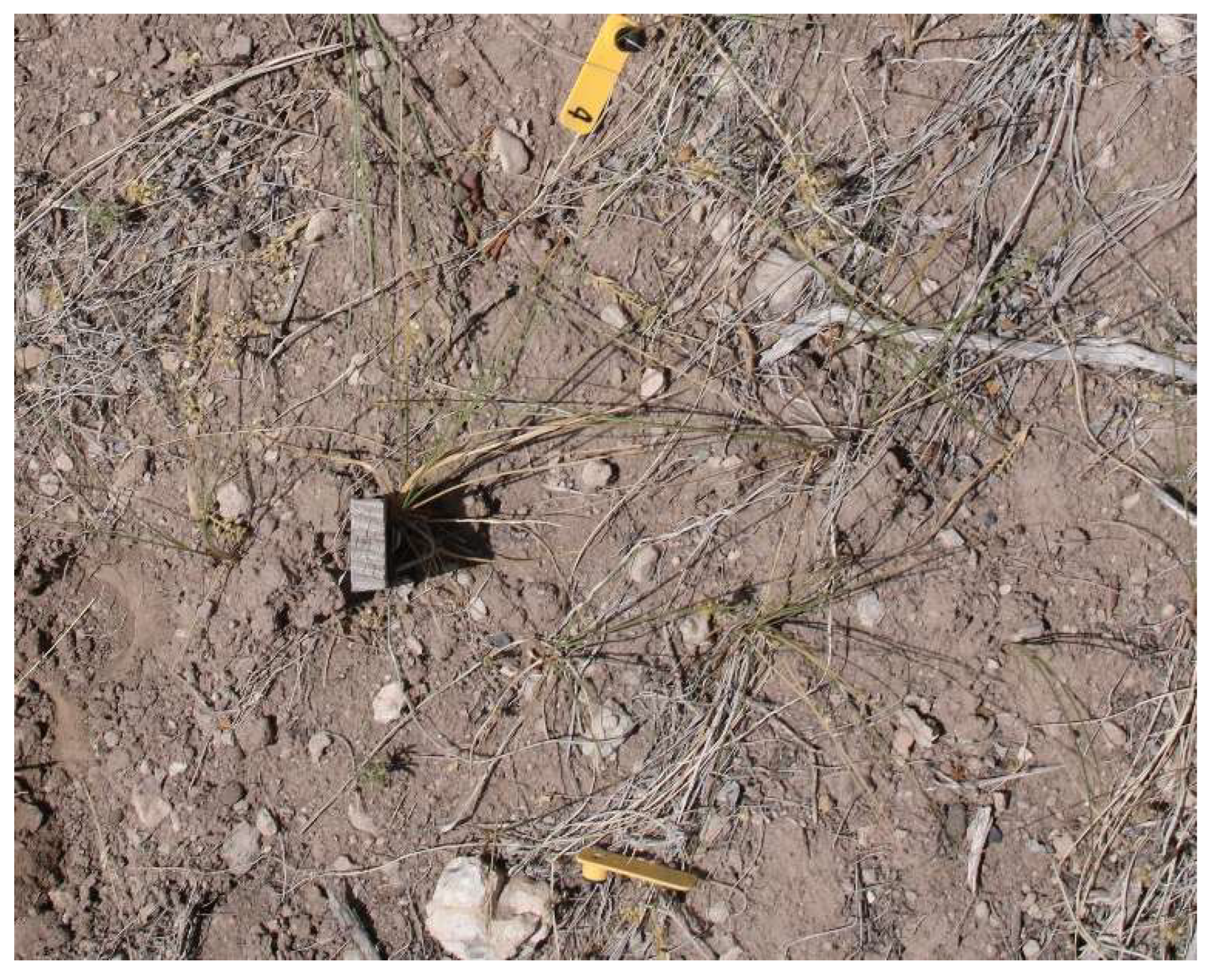
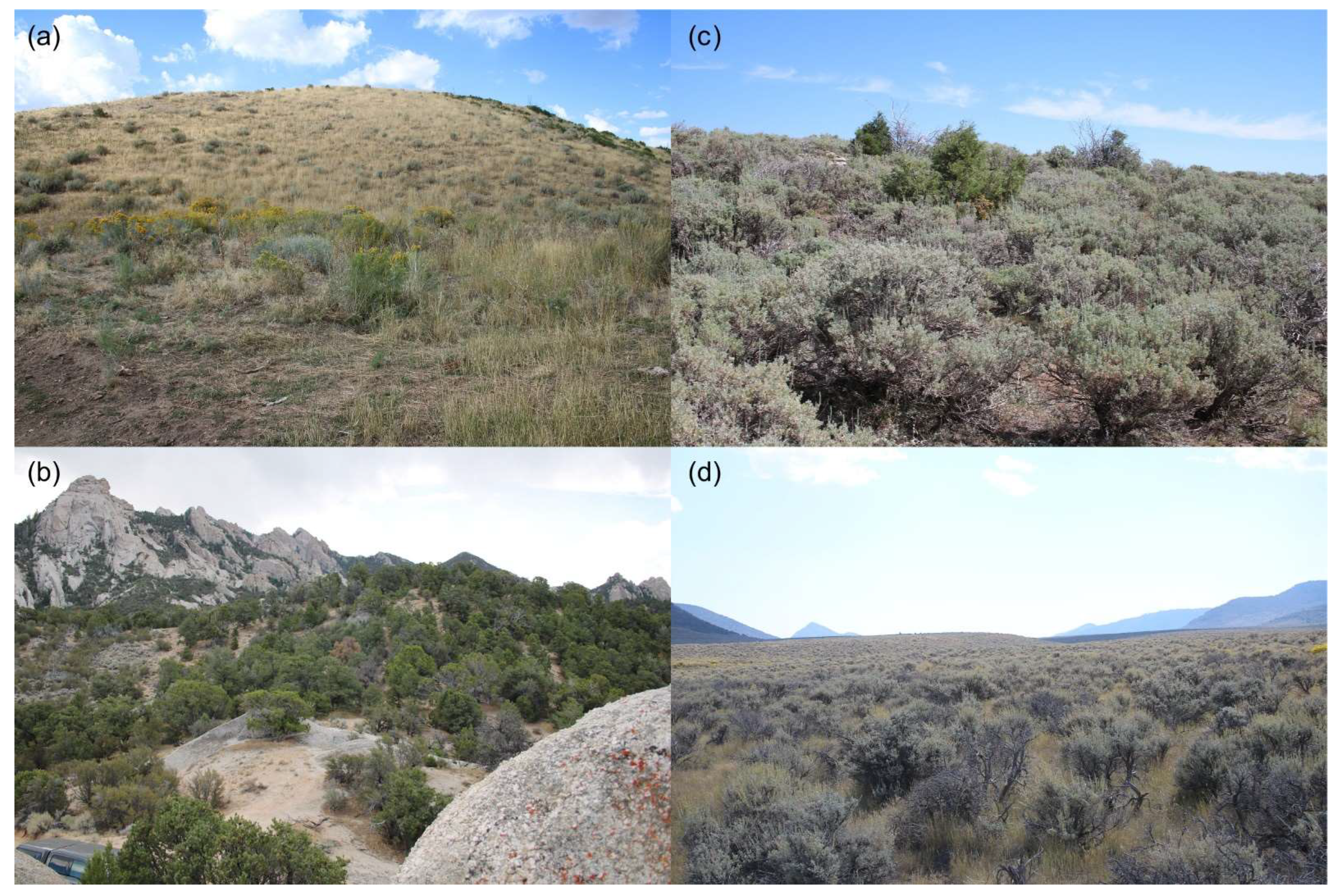
In June 2012, we set up five arrays to monitor temperature at each of two regions: a set of five arrays in the Mineral Mountains near Beaver in southern Utah and a set of five in the Uintah Mountains near Vernal in northern Utah and Colorado (although two sites were technically in Colorado, we call the latter region northern Utah; Figure 1). All sites were rangeland, where livestock graze and where Mormon crickets had been observed banding within the past five years (Figure 2). Mormon crickets are large (approximately 2 g as adults) omnivorous katydids that do not have functional wings for flight. They migrate on the ground and lay eggs in soil at approximately 2.5 cm beneath ground level. Accordingly, we monitored temperatures at approximately 2.5 cm above and below ground level (T_air and T_soil, respectively).

In each array, a wooden stake (4 × 2 × 30 cm) was erected at a central location, and a stake was placed 50 m away from the central stake in each of the four cardinal directions (Figure 1). Recording T_air and humidity, a hygrochron ibutton (DS1923, Maxim Integrated, San Jose CA, USA; diameter 15 mm, height 6 mm) on a plastic fob was screwed to the north side of the stake 2.5 cm above ground level. Recording T_soil, a thermochron ibutton (DS1922) on a plastic fob was attached to the stake with a 38 cm wire and buried the length of the wire away at 2.5 cm beneath the surface. For each stake, latitude, longitude, and elevation were recorded (Topcon GPS with sub-meter accuracy), the steepest slope of a 10 × 4 × 165 cm wooden board centered at the stake was measured with an inclinometer (Ranger 15T, Silva-USA, Sandy, UT, USA), and the aspect of the slope was classified to eight magnetic compass points (declination ca. +10°). In total, there were 25 air sensors and 25 soil sensors placed in southern Utah and 25 of each placed in northern Utah. T_air and T_soil were logged at 7700 s, the maximum rate to record one year of data before overwriting. Sensors were downloaded annually in September for five years in southern Utah. Arrays in northern Utah were downloaded annually for nine years and continue to be monitored.

A proportion of ibuttons stopped logging each year because of corrosion, battery failure, and other causes, resulting in loss of the data for the entire year. In 2016, 46% of the ibuttons had stopped logging, and we did not analyze data for that year because of the gaps. We also terminated the arrays in southern Utah in September 2016. Occasionally, stakes broke, or soil monitors came out of the ground, typically due to livestock activities or thawing. We inspected the data and compared them to neighboring sensors to determine anomalies indicating when the accident occurred, and, when we felt confident, we recovered data prior to the accident. As both southern and northern Utah were monitored between 2011 and 2015, we analyzed data from those years separately from data collected in 2017–2020 when only northern Utah was monitored.

2.2. Modeling T_air and T_soil

T_air and T_soil at each stake were modeled with NichMapR version 3.2.0 [11,16]. For the base model, we entered the latitude, longitude, elevation, slope, and aspect of each site into the NichMapR package using the micro_usa() function. For T_air, we set the height to 2.5 cm. Other parameters were set to default values, including no shading by surrounding topography, hydraulic properties of loam-textured soil, and surface reflectivity of 0.15 [16]. We lacked slope at four sites, which were set to 0. Output included T_air, T_soil at 0 and 2.5 cm, and snow depth each hour. In order to compare the modeled temperatures with empirical data that were collected less frequently, we used linear interpolation to estimate modeled temperature at the empirical time. We then calculated the root mean square deviance (RMSD_base) between modeled and empirical data sets. We also applied least-squares regression to relate empirical to modeled temperatures and report the intercept, slope, and variance explained (R²). In order to determine whether the two measures of deviance were directly proportional, we correlated the intercepts with RMSD_base.

2.3. Additions to the Base Model

Using the elevatr() package in R (v. 4.0), we used elevatr::get_elev_raster to collect a 5 × 5 raster around each stake. Digital elevations were extracted from the raster at 1/3 arc second or approximately 10 m resolution. Vertical accuracy of the digital elevation model was 0.35 m when compared with LIDAR surveyed points [17]. Slope and aspect were calculated using these small rasters at each stake with the raster::terrain() command.

Using the same 5 × 5 raster, we adjusted the base model at each stake for topographic shading by local features. Horizon angle was calculated at each of 36 compass points (every 10°) using the digital elevation at the stake and the elevation of the surrounding raster points. From these 36 points, the horizon angles at 24 compass points were interpolated and added to the ‘hori’ parameter in micro_usa. The RMSD between empirical and modeled temperatures (RMSD_hori) was calculated and compared with RMSD_base.

For each stake, we adjusted the base model for five soil parameters downloaded for Utah and Colorado (for the two sites in Colorado located a few km east of the Utah state border) from the SSURGO database of the National Resources Conservation Service (usda.nrcs.gov). The map unit key (mukey) closest to each stake was extracted using the soilDB::SoilWeb_spatial_query command. From the nearest soil horizon data, a weighted mean of each soil parameter for the top 10 cm of the horizon was calculated and added to nichMapR: albedo (called REFL in micro_usa), bulk density (BD), air entry potential (PE), saturated conductivity (KS), and Campbell’s soil b (BB). For calculating RMSD with the soil parameters (RMSD_soil), we focused on one site per array, except for one array, at which we modeled all five sites. RMSD_soil was compared with RMSD from the base model.

In the base model, roughness length was 0.004 m, which was an intermediate value for tilled soils (0.002 to 0.006 m [18]). Sagebrush, which was found on all of the arrays in northern Utah, had a roughness length of 0.02 m [19]. The roughness length for grasses was also 0.02 m for a canopy of 0.07 to 0.14 m [20], which was a reasonable range of heights for the grasses that dominate arrays in southern Utah. Hence, we modeled the air and soil temperatures with a roughness length of 0.02 m, calculated the RMSD (RMSD_ruf), and compared these with RMSD_base for both soil and air.

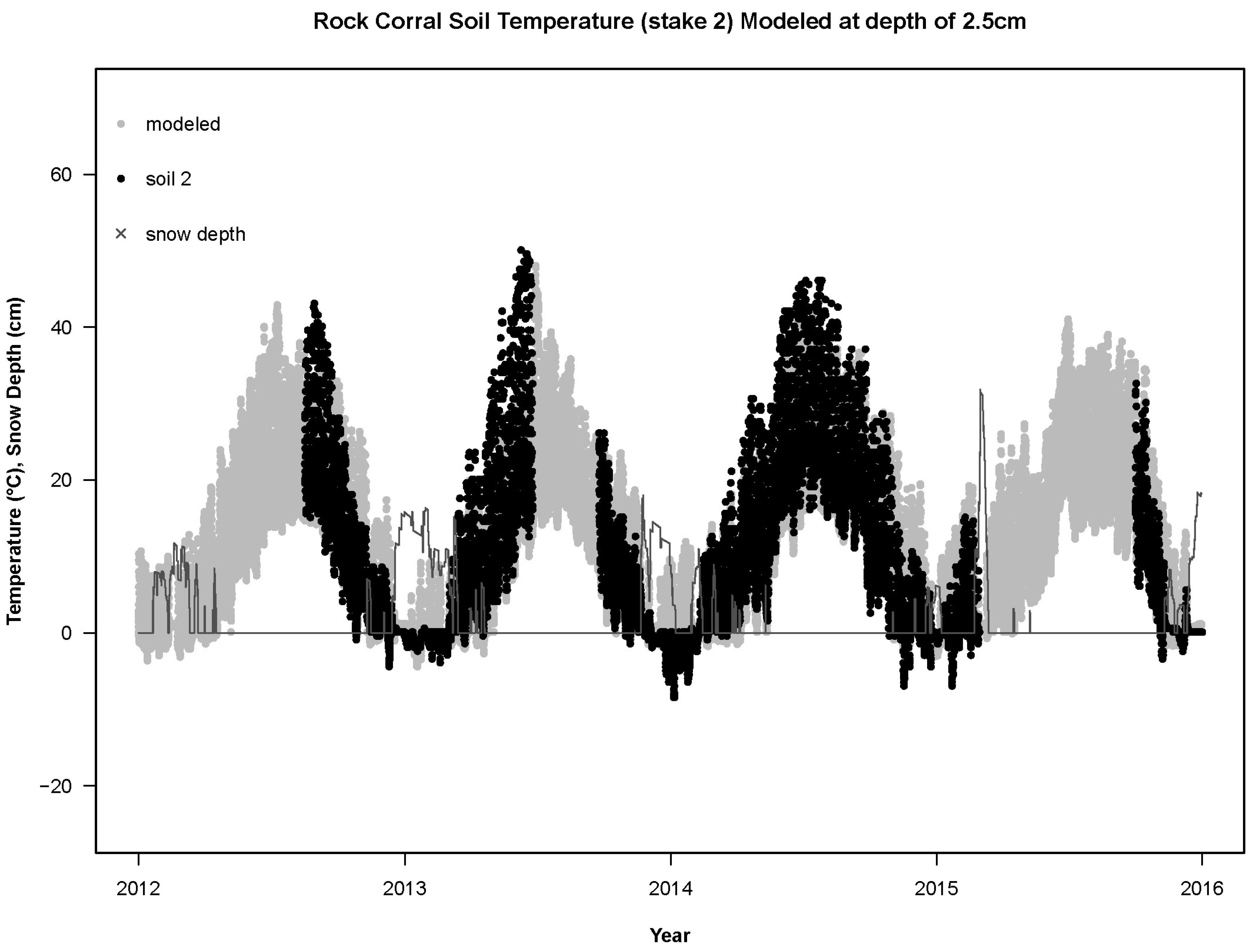
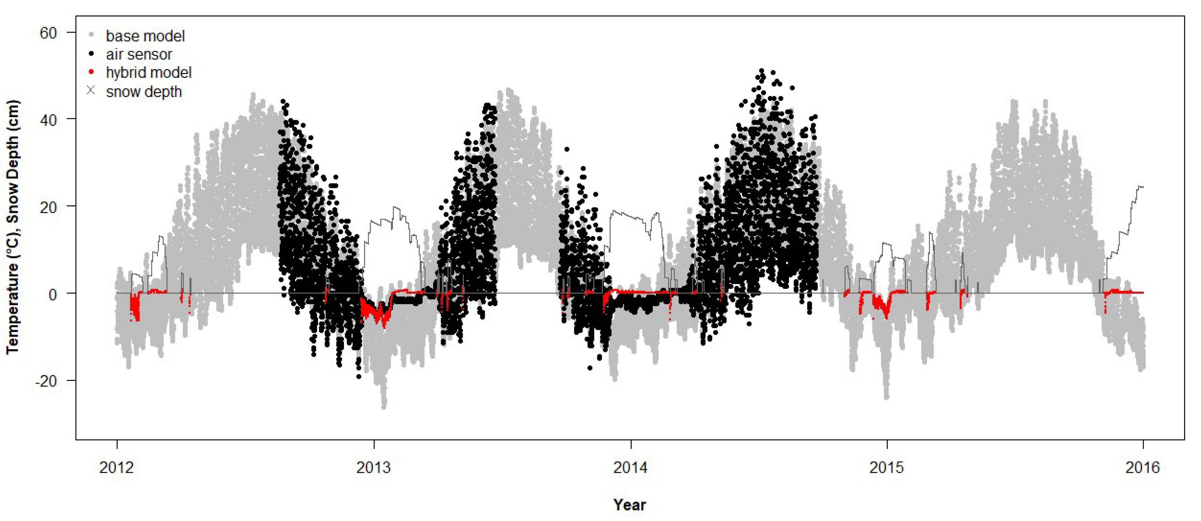
NichMapR accounted for snow depth when modeling T_soil but not T_air. We created a hybrid model that replaced T_air at 2.5 cm with T_soil at 0 cm depth when the snow depth output from NichMapR was 3 cm or greater (i.e., sufficient to cover the sensor). RMSD between empirical and modeled temperatures (RMSD_hybrid) was then calculated and compared with RMSD from the base model.

3. Results

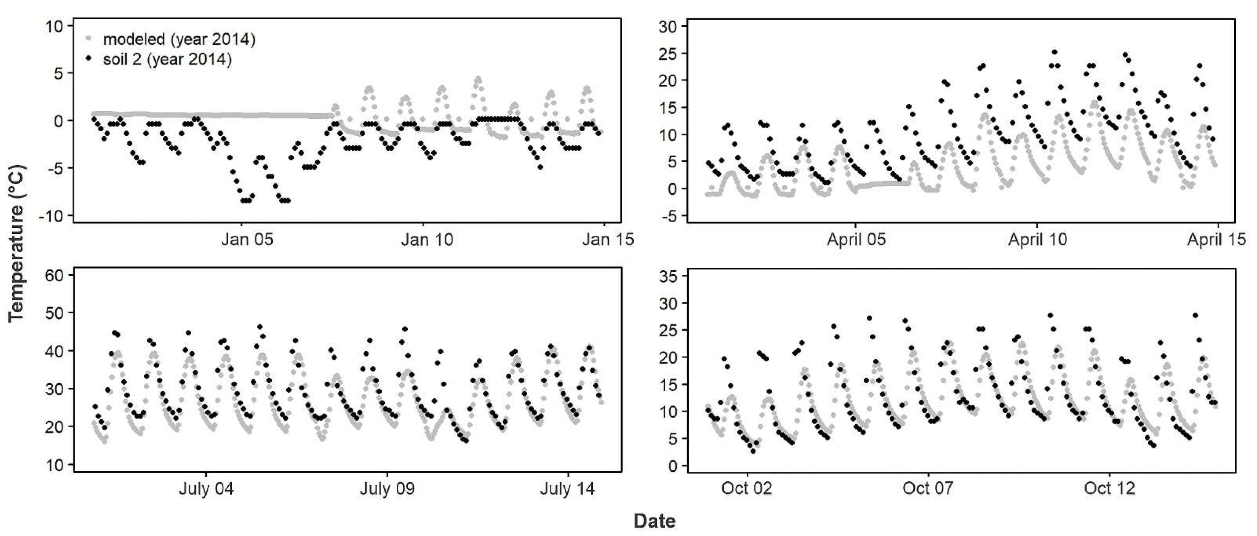
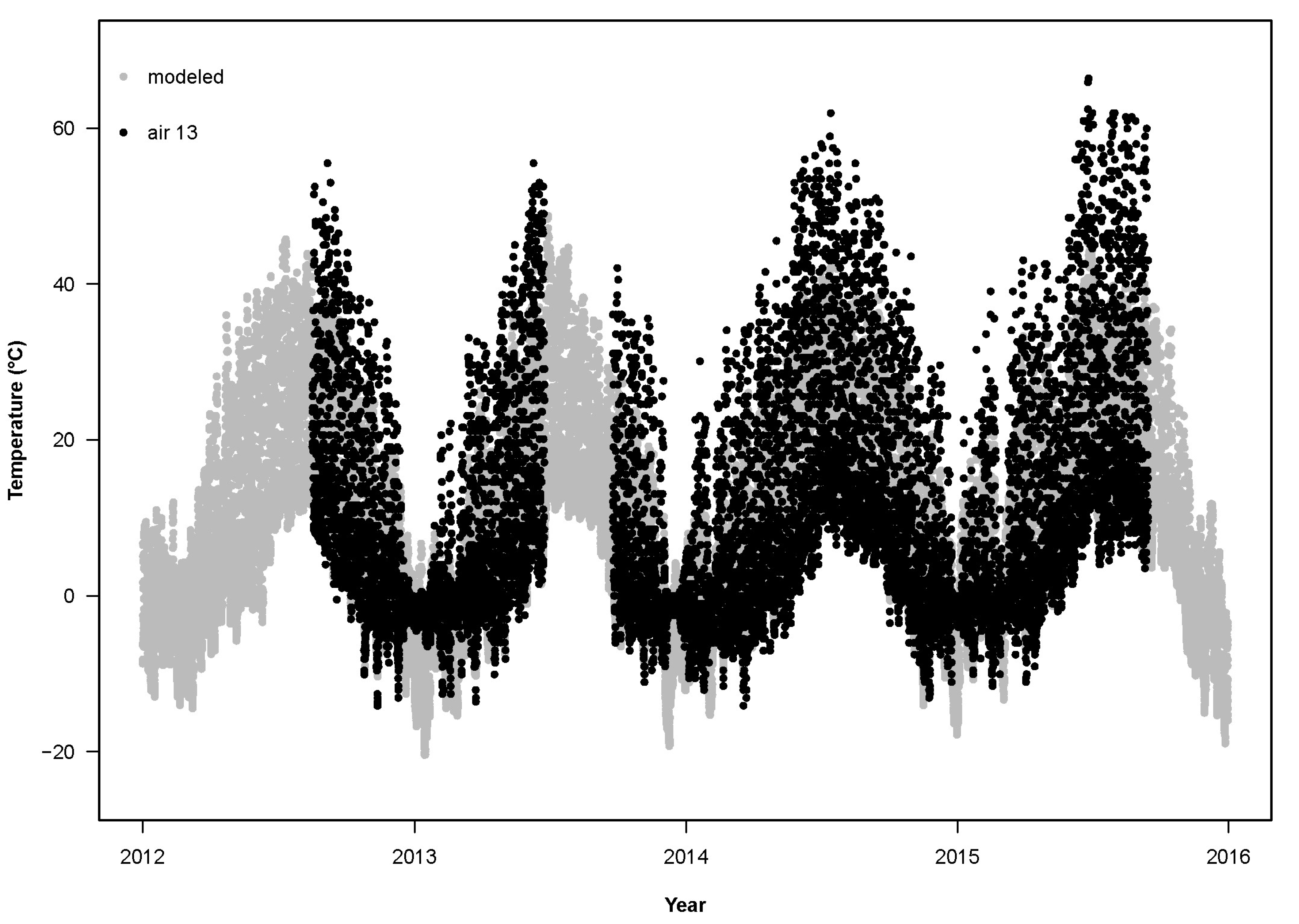
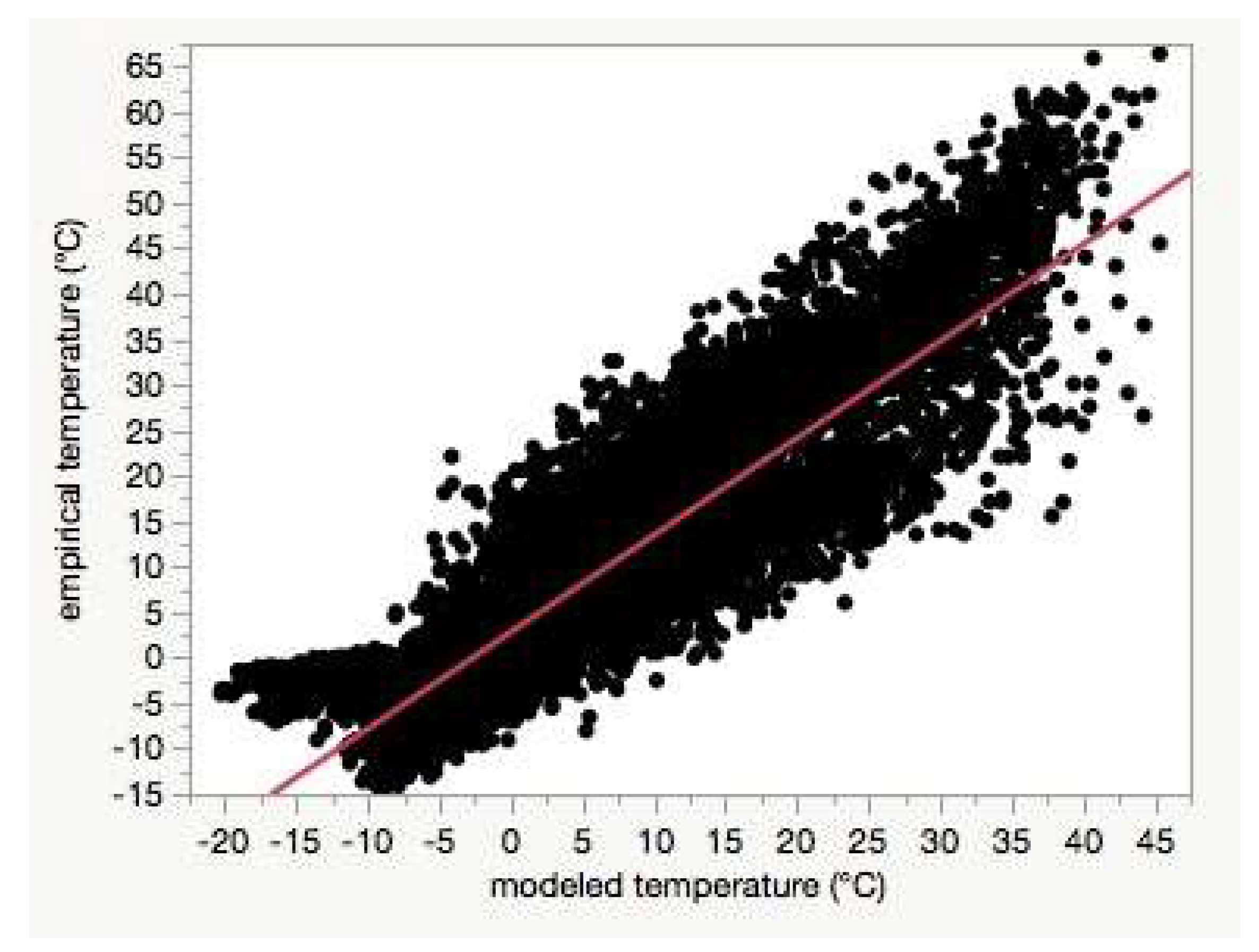
For the years 2012–2015, the RMSD between the sensors and the base model (RMSD_base) was not significantly different from a normal distribution (Shapiro–Wilk W = 0.97, p = 0.0501). 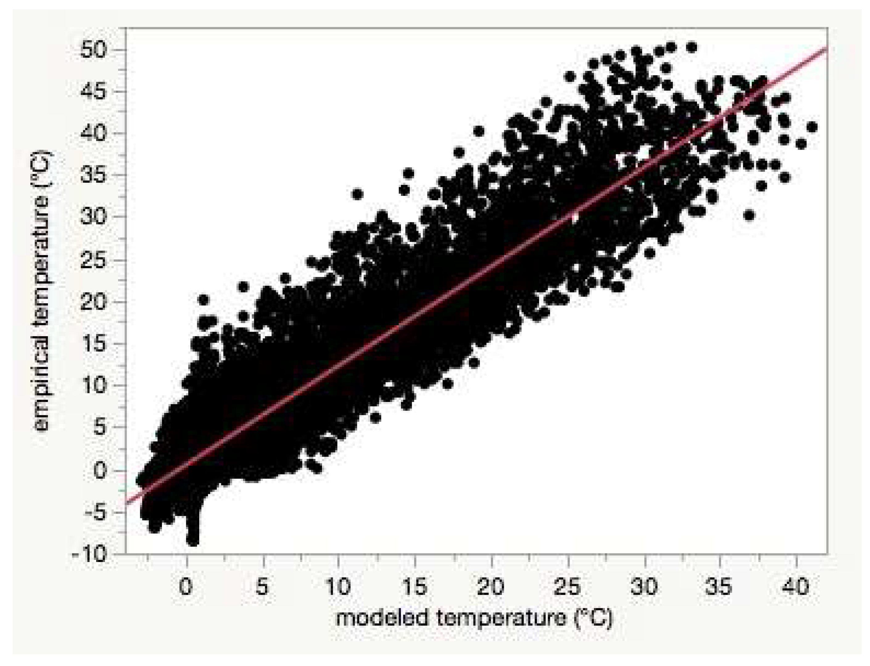The empirical T_air differed from the modeled T_air (Figure 3, Figure 4 and Figure 5) by more than the empirical T_soil differed from the modeled T_soil (F_1,84 = 148.8, p < 0.0001; average RMSD_base for T_air: 7.4 °C, n = 49; for T_soil: 4.4 °C, n = 37; Figure 6, Figure 7 and Figure 8). Using least-squares regression to estimate the linear relationship between empirical and modeled air temperatures for each site (e.g., Figure 4), the RMSD_base was positively correlated with the intercepts (Pearson’s r = 0.67, p < 0.0001, Table S1).

3.1. Effects of Digital Elevation Model Estimates of Slope and Aspect

The RMSD with the digital elevation model measurements of slope and aspect (RMSD_DEM) was not significantly different from a normal distribution (n = 20, Shapiro–Wilk W = 0.95, p = 0.41). The RMSD_DEM was not affected by whether the sensor was in air or soil (ANCOVA, F = 0.3, p = 0.59) and resulted in very little change relative to the RMSD of the base model (RMSD_DEM = 0.20 + 0.98 × RMSD_base, R² = 0.99, p < 0.0001). Although the slope derived from the digital elevation model (DEM) increased less steeply than the slope measured locally (slope_DEM = 2.4 + 0.4 × slope_local), the modeled temperatures constructed with digital elevations measured remotely were not much different than those modeled with ground measurements of the slope and aspect.

3.2. Shading Effects Due to Surrounding Topography

The RMSD for the horizon modification to the base model (RMSD_hori) was significantly different from a normal distribution (n = 86, Shapiro–Wilk W = 0.97, p = 0.045). Thr RMSD_hori resulted in very little change relative to RMSD_base for both T_air (RMSD_hori = −0.12 + 1.01 × RMSD_base) and T_soil (RMSD_hori = 0.01 + 0.99 × RMSD_base).

3.3. Effects of Soil Parameters from Empirical Soil Database SSURGO

The RMSD for the soil parameter modification to the base model was not significantly different from a normal distribution (n = 27, Shapiro–Wilk W = 0.96, p = 0.48). The RMSD for the soil parameter modification (RMSD_soil) was significantly related to the RMSD_base (F = 54.2, p < 0.0001) and also affected by the sensor location (F = 13.6, p = 0.0011; air: 8.0, soil: 9.6 °C). Incorporating mapped soil parameters made modeled temperatures less similar to empirical data than the base model, with the relation between modeled soil temperature and empirical data particularly worsening (on average, T_air models were 19% poorer, whereas T_soil models were 86% poorer than the RMSD_base model).

3.4. Effects of Roughness Length

For the years 2012–2015, the RMSD between the sensors and the temperatures modeled with the roughness length modification (RMSD_ruf) was not significantly different from a normal distribution for air or soil (Shapiro–Wilk W = 0.97, p > 0.31). The RMSD_ruf resulted in very little change relative to the RMSD_base for both T_air (RMSD_ruf = −0.23 + 1.07 × RMSD_base) and T_soil (RMSD_ruf = −0.02 + 0.99 × RMSD_base). On average, the RMSD_ruf was 0.3 °C (3.7%) poorer for air temperature and 0.1 °C (1.7%) improved for soil temperature relative to RMSD_base.

3.5. Effects of Snow on Air Temperature

The RMSD for the hybrid modification to the base model (RMSD_hybrid), which only modified T_air, was not significantly different from a normal distribution (n = 49, Shapiro–Wilk W = 0.99, p = 0.98). The RMSD_hybrid was linearly related to RMSD_base and showed an improvement of 8% on average (RMSD_hybrid = 1.09 × RMSD_base −1.23, R² = 0.82, p < 0.0001). Forty-two sites saw an improvement between model temperature and empirical T_air, with the greatest change in the RMSD being 31% (Figure 9), whereas only seven sites saw agreement between model temperature and empirical T_air worsen, with the greatest by 9% (Figure 10). Both the RMSD_hybrid for T_air and the RMSD_base for T_soil were independent of the sample size (p = 0.652 and 0.961, respectively). The RMSD_hybrid was positively correlated with the intercept of the regression of empirical temperature on the hybrid-modeled T_air (Pearson’s r = 0.57, p < 0.0001).

As the hybrid model resulted in a substantial improvement in the simulated T_air data, we investigated the effects of aspect and slope on model and empirical data agreement using the RMSD_hybrid for T_air and the RMSD_base for T_soil. The aspect was categorized into four compass points: 316–45° = N, 46–135° = E, 136–225° = S, and 226–315° = W. For 2012–2015, the RMSD_base was directly proportional to slope, whereas the RMSD_base did not vary among aspects (ANCOVA: slope F_1,21 = 10.8, p = 0.0035; aspect F_3,21 = 0.67, p = 0.578; after interaction p = 0.39 was pooled with error). The addition of flat areas as a fifth category did not change the result qualitatively (slope F_1,29 = 8.6, p = 0.0064; aspect F_4,29 = 0.58, p = 0.678, interaction pooled with error). The RMSD_hybrid was independent of slope, whereas it was significantly affected by the aspect (ANCOVA: slope F_1,30 = 0.34, p = 0.567; aspect F_3,30 = 4.50, p = 0.010; after interaction p = 0.58 was pooled with error). The post hoc multiple comparison of the means indicated that the empirical and modeled T_air agreed best on the northern aspects and worst on the eastern aspects (E^a = 7.8, W^a = 7.2, S^a = 6.9, N^b = 5.8 °C). The addition of flat areas resulted in the RMSD_hybrid being independent of the slope and aspect (ANCOVA: slope F_1,39 = 0.54, p = 0.468; aspect F_4,39 = 2.52, p = 0.056; interaction pooled with error).

For 2017–2020, the RMSD_hybrid model showed improvement over the RMSD_base at 22 of the 25 sites (RMSD_hybrid = 1.10 × RMSD_base − 1.42, R² = 0.92, p < 0.0001). By combining aspects into four compass points, we found that neither the RMSD_base for T_soil nor the RMSD_hybrid were significantly affected by slope or aspect (ANCOVA, RMSD_base: slope F_1,14 = 0.27, p = 0.849, aspect F_3,14 = 0.02, p = 0.882, interaction p = 0.404 pooled with error; RMSD_hybrid: slope F_1,14 = 0.57, p = 0.642, aspect F_3,14 = 1.87, p = 0.192, interaction p = 0.702 pooled with error). The addition of flat areas as a fifth class did not qualitatively alter these results.

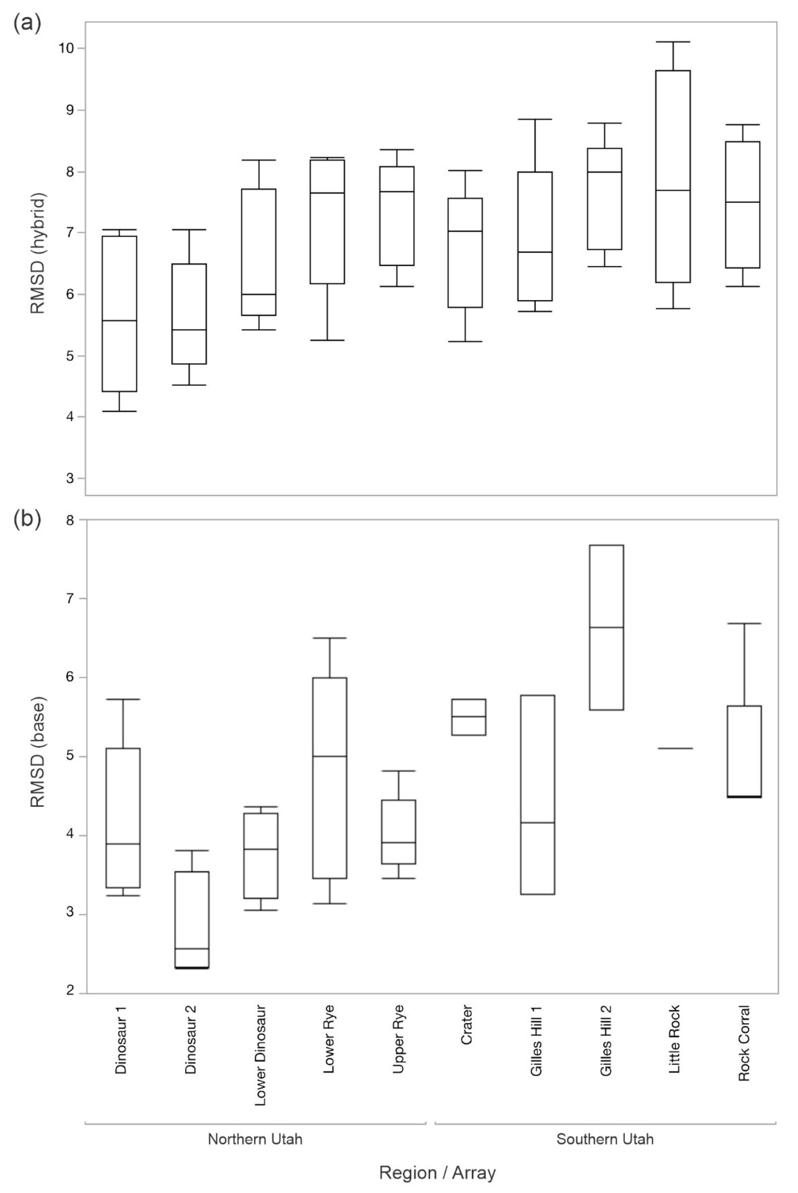
For 2012-2015, the RMSD_hybrid was significantly different among the topographic assemblage as defined by the array of sensors (F_9,39 = 2.16, p = 0.0469). Little Rock had the greatest RMSD_hybrid and Dinosaur 2 the least (Figure 11). The arrays were significantly different in the RMSD_base for T_soil (F_9,27 = 3.67, p = 0.0041), with Gilles Hill 2 having the greatest RMSD and Dinosaur 2 the least (

Table 1. RMSD_hybrid for air temperature and RMSD_base for soil temperature for two four-year time periods are compared among arrays located in Utah.

Region	Array	Mean RMSDhybrid 2012–2015 *	Mean RMSDbase 2012–2015 *	Mean RMSDbase 2017–2020 *
Northern Utah	Dinosaur 1	5.66 b	4.21 a,b,c	5.12 a,b
Northern Utah	Dinosaur 2	5.63 b	2.93 c	5.37 a,b
Northern Utah	Lower Dinosaur	6.54 a,b	3.83 b,c	5.76 a,b
Northern Utah	Upper Rye	7.36 a	4.07 a,b,c	6.69 a
Northern Utah	Lower Rye	7.27 a	4.83 a,b,c	4.04 b
Southern Utah	Gilles Hill 1	6.90 a,b	4.45 a,b,c
Southern Utah	Gilles Hill 2	7.64 a	6.67 a
Southern Utah	Crater	6.75 a,b	5.54 a,b,c
Southern Utah	Little Rock	7.88 a	5.14 a,b,c
Southern Utah	Rock Corral	7.47 a	5.00 a,b

* Different superscripts indicate significant differences among the means in post hoc comparisons.

). For 2017–2020, there was no significant relation between the RMSD_hybrid and the array (F_4,20 = 1.42, p = 0.265), but the arrays were significantly different in the RMSD_base for T_soil (F_4,20 = 3.85, p = 0.0187). Upper Rye had the greatest RMSD and Lower Rye the least (Table 1).

4. Discussion

Many organisms are affected by temperatures within 2.5 cm of the Earth’s surface both above and below ground [21,22]. Physical modeling of near-surface temperature between weather stations is logistically feasible, but we found that empirical data from two regions of Utah and Colorado differed from temperature data modeled with NichMapR by an average of 7.4 °C for air temperature and 4.4 °C for soil temperature. The modification of default parameters resulted in little improvement in error, suggesting that the modeled temperatures were remarkably insensitive to changes. The incorporation of snow cover into the modeled T_air generally made the modeled data more similar to the empirical temperatures (an average difference of 6.9 °C). These hybrid models were the most effective when NichMapR accurately modeled snow depth. In addition to regional variation in snowfall, snow depth was also affected by drift and other sources of wind-induced error. Topographic variation undoubtedly affected snow accumulation and melting.

The difference between the empirical and modeled temperatures was larger in T_air than T_soil. In early morning and late evening hours when the air sensor was not in the shade provided by the stake, heating of the silver metal sensor housing by sunlight [23] would introduce error to the empirical T_air but not T_soil and potentially contribute to the 2.5 °C difference in RMSD between the hybrid model for T_air and that for T_soil. As an aside, ground surface temperatures can be extremely inhospitable to an insect. In the tracking of a migratory band of Mormon crickets in Nevada in June 2008 [24], surface temperature, measured with an Omega thermocouple thermometer, exceeded 50 °C when the ambient temperature at 1.5 m above ground was only 28.3 °C and reached 59.6 °C when ambient temperature was 31.8 °C. These hand-collected data support the maximum temperatures recorded by the air sensors in Utah, which occasionally exceeded 60 °C (Figure 3, Figure 4 and Figure 10).

For the years 2012–2015, the empirical and modeled T_air were most alike on the northern aspect, where shading was greatest. In contrast, errors in T_soil increased with slope, which might have resulted from some loss of soil over the sensor due to erosion. Contrarily, these differences may have been due to the adverse effects of the slope and aspect on the accuracy of the modeled data themselves. Differential effects of the slope and aspect on T_soil and T_air, whether modeled or empirical, may explain why the RMSD_base for T_soil was not associated with the RMSD_hybrid for T_air (n = 36, r = 0.264, p = 0.12).

The shading from vegetation may have also contributed to differences between the empirical and modeled temperatures. In addition to the modeled temperatures, assuming 0% vegetation cover that we reported, NichMapR generated an output for 90% vegetation cover. However, most of the sites that we sampled were sparse in vegetation and were much nearer to the assumption of 0% cover. Even sagebrush and juniper (e.g., Figure 2) were spaced so that the canopy over the sensors was typically open. The average area of bare ground in a 50 × 50 cm square encompassing the air and soil temperature sensors in northern Utah was 81% (Figure 12). Although the temperature for vegetation cover in between 0 and 90% cover could be calculated by interpolation, the addition of any vegetation cover would decrease the modeled temperature and thus increase the RMSD between the modeled and empirical temperatures. The canopy photos that track the sun’s path provided precise measurements of incident sunlight, but we did not deem those to be necessary in the sparse vegetation.

In understanding the role of topography in climate refugia, modeled data would be the least biased if slope or aspect had no effects on their agreement with the empirical temperatures. Differences between empirical and modeled data for the years 2017–2020 were not affected by slope or aspect. Similarly, when flat areas were included in the empirical and modeled data for the years 2012–2015, neither slope nor aspect affected the RMSD_hybrid or RMSD_base, respectively. Hence, over a broadened topography, modeled temperatures were unbiased by slope and aspect in two discrete, four-year time spans.

For the years 2012–2015, the difference between the empirical and modeled soil temperature was greatest at Gilles Hill 2 and least at Dinosaur 2. These two sites also had significantly different RMSD_hybrid, with Dinosaur 2 being the lesser. The two topographic assemblages were very different: Gilles Hill 2 is a mountain grassland on volcanic soil in southern Utah, whereas Dinosaur 2 is a rocky outcropping on sedimentary soil in Dinosaur National Monument. The sites at Gilles Hill 2 face north or south, with steep slopes between 20 and 21°, whereas those in Dinosaur 2 face north or south, with shallower slopes ranging between 0 and 8°. For the years 2017–2020, Upper Rye had the greatest difference between empirical and modeled soil temperature, and Lower Rye had the least. However, these two topographic assemblages are very similar; both are relatively flat (facing east, south, or west from 0–7° for Lower Rye and facing east or south from 0–6° for Upper Rye), dark-soil grasslands interspersed with sagebrush on the Diamond Plateau in northern Utah, which makes the difference in the RMSD_base difficult to explain.

Despite the differences in the modeled and empirical temperatures that we highlighted over a nearly ten-year time period in Utah, the advantages of the modeled data far outweighed the inaccuracies when modeling demographics, range shifts, and other events on a regional scale. For example, the Mormon cricket outbreak of the first decade of this century encompassed 7.2 million acres, an area the size of West Virginia, spread over six states in the western United States [25,26], and it is not yet possible to measure near-surface microclimate on that broad a spatial scale. However, an understanding of biological phenomena will be much more accurate with empirical measures of T_air and T_soil by an array of sensors on a local scale and the near-surface empirical data expanded to landscape and regional scales with the remote sensing of topography [27]. For example, we are currently investigating the egg diapause of Mormon crickets, which can be prolonged for several years (Figure 12, [28,29]), while simultaneously measuring T_air and T_soil with the sensor arrays in northern Utah and Colorado described in this paper. Empirical temperatures give the most accurate measurements of heat accumulation over time for predicting temperature-dependent biological processes, such as degree days for egg development in soil. Despite differences with empirical temperatures, temperatures modeled with nichMapR at the height of the organism are much more accurate than simply using temperatures from weather stations at 1.5 to 2 m above the ground surface for calculating degree–day accumulation.

Future projections of spatial and temporal variations in microclimate availability can only be modeled from macroclimate projections. In order to understand the ecological consequences of climate change, biophysical models that downscale climate to ecologically relevant spatial and temporal scales need to be created to understand changes in niche structure [30]. To achieve the widest applications possible, biophysical models need to be validated with empirical data from a wide variety of altitudes, latitudes, soil types, topographies that organisms currently inhabit, and where their ranges might expand to in the future. This study of two regions of Utah contributes to that effort.