Article

Comparison between Parametric and Non-Parametric Supervised Land Cover Classifications of Sentinel-2 MSI and Landsat-8 OLI Data

by
Giuseppe Mancino
1,*,
Antonio Falciano
1,
Rodolfo Console
1,2 and
Maria Lucia Trivigno
1
1
Centro di Geomorfologia Integrata per l’Area del Mediterraneo (CGIAM), Via F. Baracca 175, 85100 Potenza, Italy
2
Istituto Nazionale di Geofisica e Vulcanologia (INGV), Via di Vigna Murata 605, 00143 Roma, Italy
*
Author to whom correspondence should be addressed.
Geographies 2023, 3(1), 82-109; https://doi.org/10.3390/geographies3010005
Submission received: 24 November 2022 / Revised: 5 January 2023 / Accepted: 8 January 2023 / Published: 12 January 2023
(This article belongs to the Special Issue A GIS Spatial Analysis Model for Land Use Change (Volume II))

Abstract

:
The present research aims at verifying whether there are significant differences between Land Use/Land Cover (LULC) classifications performed using Landsat 8 Operational Land Imager (OLI) and Sentinel-2 Multispectral Instrument (MSI) data—abbreviated as L8 and S2. To comprehend the degree of accuracy between these classifications, both L8 and S2 scenes covering the study area located in the Basilicata region (Italy) and acquired within a couple of days in August 2017 were considered. Both images were geometrically and atmospherically corrected and then resampled at 30 m. To identify the ground truth for training and validation, a LULC map and a forest map realized by the Basilicata region were used as references. Then, each point was verified through photo-interpretation using the orthophoto AGEA 2017 (spatial resolution of 20 cm) as a ground truth image and, only in doubtful cases, a direct GPS field survey. MLC and SVM supervised classifications were applied to both types of images and an error matrix was computed using the same reference points (ground truth) to evaluate the classification accuracy of different LULC classes. The contribution of S2′s red-edge bands in improving classifications was also verified. Definitively, ML classifications show better performance than SVM, and Landsat data provide higher accuracy than Sentinel-2.

1. Introduction

The Earth’s study by using remote sensing technologies has acquired more and more importance in recent decades, and, at present, most of the payloads of the new satellite missions are equipped with dedicated sensors for Earth observation (EO), enabling the scientific community to take advantage of these data sources for a wide range of application fields. The remote sensing images coming from satellite sensors allow us to obtain a global view of the Earth, with the possibility of observing and studying even very remote and inaccessible areas of the globe, where classical investigations would be extremely onerous if not impossible. Currently, the satellite missions for the EO purpose are numerous and diversified, and, therefore, they have review times in the same area remarkably close together, with the possibility of the continuous monitoring of natural and anthropic phenomena [1,2].
Scientific research has considerably expanded the areas of application of remote sensing thanks to the different spectral, geometric, and temporal resolution characteristics of airborne and satellite sensors. The sectors range from morphological ones (realization of digital elevation models—DEM, digital surface models—DSM, topography, etc.) to geological ones (recognition of rock types, soil studies, monitoring of degradation phenomena such as landslides, erosion, desertification, etc.) [3,4,5], from the study of the quality of lakes [6,7] and the dynamism of inland waters [8] to oceanography studies [9]. Applications also concern land consumption (urban sprawl, urban structure and density, detection of unauthorized constructions, road infrastructures) [10,11], the monitoring and management of natural and anthropogenic disasters (earthquakes, hurricanes, landslides, wildfires, pollution, etc.), biochemical processes [12], and the monitoring of the conservation levels of monumental and archaeological sites [13].
Agriculture and forestry represent historical remote sensing fields, which are still expanding [14,15]. The first concerns various sectors ranging from crop classification and phenological cycles to the presence of water stress, infestations, etc. [16,17]. In the forestry sector, the fields of application are very broad and range from forest species classification to vegetation dynamics, forest recolonization processes, deforestation [18,19,20], the identification of tree biomass, and other forest variables [21,22]. Further areas of investigation in forestry are net primary production [23,24,25], forest plantations [26], fire monitoring and detection [27] and the characteristics of wildfires [28,29], and anthropogenic stress on the environment [30].
One of the application fields of remote sensing, historically the most dated and widely used, concerns the realization of LULC maps. Recently, LULC maps have become increasingly important in various sectors, including sustainable land management, landscape ecology, research on climate change, etc. [31,32,33]. Land Use and Land Cover Change (LULCC) maps help us to better understand the environmental processes related to the water cycle, biochemical cycles, and energy exchange. Moreover, they represent a piece of important information to better understand the biodiversity alterations and the presence of environmental stresses possibly related to natural or anthropic factors. Land cover has also been recognized as an Essential Climate Variable (ECV) and proposed as a Satellite Remote Sensing Essential Biodiversity Variable [34]. Land cover characterization with high thematic and spatial levels (spatial resolution less than or equal to 30 m) allows the Earth’s surface monitoring on a comparable scale to that of human activity [35].
In recent years, there has been an explosion in the availability of remote sensing data at medium–high resolution mounted on different platforms, and, at the same time, the methods and techniques for the realization of land cover maps have been refined and expanded. The realization of LULC maps through remote sensing involves a series of phases, including the selection of the remotely sensed data (mission, sensor, spectral bands, etc.), the identification of ground truth for the application of the classification algorithm, and ground surveys for the validation of the method and the possible selection of the algorithm that has the best performance. In the literature, there are many studies on LULC classification techniques through the use of supervised and unsupervised algorithms, per-pixel or object-based [36,37].
A meta-analysis of pixel-based supervised techniques for land cover classification performed by Khatami et al. [38] reveals that the inclusion of ancillary data, textures, and multitemporal images allows for a significant improvement in the accuracy of the classification. However, ancillary data are not always available and the processing of multitemporal data requires greater accuracy in data processing and a much higher investment in terms of time and human resources. Furthermore, as shown in the work of Khatami et al. [38], the most efficient contribution to the improvement of the goodness of the classification is provided by the texture. In recent years, also as a consequence of the effects of climate change, land use has tended to change very rapidly [39], so it is often necessary, for the correct management of natural resources, to provide updates with very close temporal steps. Among other factors, the traditional techniques that involve continuous field surveys turn out to be very onerous [40]. Moreover, the maps of LULC and LULCC made on a global scale or for very large geographical areas (continental and even national), using the data [41,42] of satellites for EO, turn out to be of insufficient precision (considering the very wide geographic scope) and accuracy (as a consequence of the resolution of the minimum mapped unit). The resolution of the pixel appears to be excessively broad in these areas and for these sensors, so the percentage of mixed pixels, i.e., areas that include more land use types, is decidedly considerable [43]. Ultimately, these products are too coarse for analysis on a local and national scale and their reliability has often been questioned [44]. Technologies based on remote sensing, however, represent the most efficient and least expensive way, considering the free availability of images, to monitor the changes that occur on Earth.
The current open availability of medium–high-resolution satellite images allows for obtaining reliable land use maps at the local or regional level and in application fields ranging from urban planning to the agricultural sector and the management of natural resources [45]. Already since 2008, the US Geological Survey (USGS) policy on open data [46] has led to a drastic increase in the use of Landsat images in the scientific community, with an ever-increasing demand for Landsat mission data over the years [39]. The launch in 2013 of the Landsat 8 satellite with OLI and TIRS sensors on board, with better spectral characteristics than those of the previous Landsat missions, has contributed to further increasing the use of these data for obtaining LULC both on a local scale and in much broader areas [47]. On 27 September 2021, the new Landsat 9 satellite was also launched into orbit, with the same optical characteristics as Landsat 8 OLI, which will therefore ensure an increase in the repetitiveness in the same area. The open data policy has also had repercussions for other space agencies. The European Space Agency (ESA) has launched satellites for EO, Sentinel-1, -2, and -3, that provide free satellite images for the scientific community, government agencies, the private sector, etc. [48,49,50]. ESA data are acquired in the microwave (Sentinel-1) and optical (Sentinel-2 and -3) electromagnetic spectrum [49]. The Sentinel-2A satellite was launched in June 2015, while Sentinel-2B was launched on 7 March 2017. Thanks to these twin satellites, a high revisit is ensured (approx. 2–3 days). The images have a swath width of 290 km and provide multispectral images in 13 bands at different spatial resolutions. They include 10 m resolution bands (four bands, three in the visible and one in the near-infrared) and 20 m resolution bands (red-edge and two bands in the short-wave infrared), as well as 60 m bands for atmospheric correction [48].
The studies comparing Sentinel-2 (S2) with Landsat 8 (L8) found that S2 improved the spatial and spectral capabilities in identifying different grassland management techniques [51], in the estimation of tree cover and the leaf area index (LAI) [52], to improve the classification quality of built-up areas [11]. These comparative studies attributed the best performance of the S2 to the inclusion of the three red-edge bands of the EM. These bands are allocated between the red and NIR bands and are characterized by an increase in the sharpness of the reflection on the vegetation [53]. Several studies have highlighted the importance of these bands in LAI estimation [53], in the identification of chlorophyll and nitrogen content in plants [54], and in the discrimination of different crop types by their sensitivity towards the structural diversity of leaves and foliage [55]. Vegetation indices have also been developed, based on the red-edge band, which has proven to be efficient for the early diagnosis of stress symptoms in forest stands, ensuring timely intervention and the protection of forest resources [56]. The inclusion of the red-edge bands in a classification scheme [57] has positively influenced the discrimination capacity of the various land use classes by improving the accuracy of the LULC classification. Previously [58], comparing the accuracy between classifications with the use of Compact Airborne Spectrographic Imager (CASI) data, with sixteen spectral bands, and Landsat TM data, it has been shown that the implementation of the red-edge band classification algorithm leads to an improvement in accuracy.
Numerous classification techniques have been developed over the years; among those that use the pixel as a basic analysis unit, there are unsupervised techniques (e.g., K-means and ISODATA) and supervised techniques (i.e., Maximum Likelihood, Minimum Distance, Artificial Neural Network, Decision Tree, Support Vector Machine, Random Forests) [40,59] and genetic algorithms [60]. Among the widely used non-parametric supervised techniques are machine learning, particularly Random Forests and SVM (Support Vector Machine) [61]. Hybrid classification techniques have also been processed [62], such as semi-supervised and a fusion of supervised and unsupervised learning.
The present study aimed to compare, using two of the most reliable classification algorithms, one parametric (Maximum Likelihood Classifier—MLC) and the other non-parametric (Support Vector Machine—SVM), the accuracy of LULC obtained from the data of the two Landsat 8 OLI and Sentinel-2 satellites. For the two sensors, the bands positioned in the same range of the electromagnetic spectrum were used, and, finally, it was verified whether and to what extent the implementation of the S2 red-edge bands leads to an improvement in the accuracy of the classification.

2. Materials and Methods

2.1. Study Area

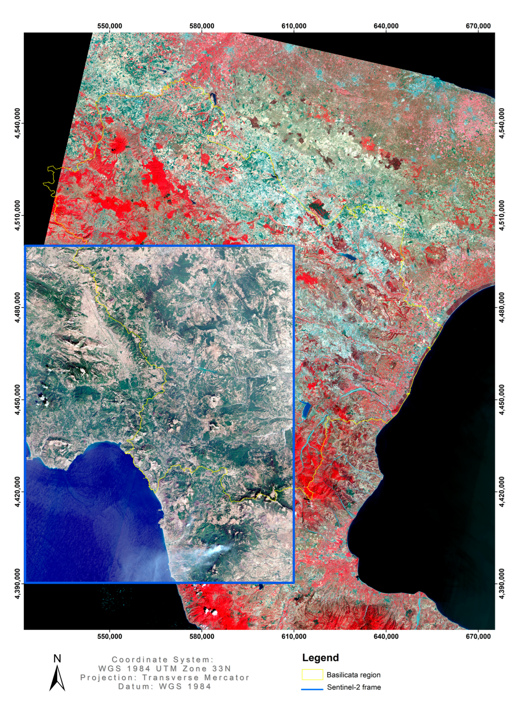
The area in question falls within the central–northern portion of the Basilicata region (Italy), also including the regional capital, and covers an area of ~36,000 ha (Figure 1). It is a large representative area, both in morphological and vegetational terms, of the hilly and mountainous landscape of Basilicata. From the orographic point of view, the area has considerable altimetric variability, with a minimum altitude value of ~546 m a.s.l. and a maximum of just over 1700 m a.s.l., with a difference in height, therefore, of over 1000 m. The most widespread altimetric range is the mountainous and high-mountainous one (over 75% of the area in question), with ~40% of the area in the range between 800 and 1000 m and ~35% over 1000 m. It is the area of the west and southwest of the study site, corresponding to the ridge of the Lucanian Apennines. Approximately a quarter of the entire surface is instead located in a hilly area, especially in the 600–800 m range. To this altimetric variability corresponds the high variability of the slopes, with areas of approx. 20% with slopes greater than 45°. The slope values are, however, generally high, and the flat or sub-flat surfaces (i < 5°) affect approx. 5% of the entire study area. The morphological and therefore climatic variability corresponds to the variability of land uses.
The area is mainly occupied by forest types, which affect over 65% of the entire study site. There are mainly broad-leaved forests (~50% of the entire area) and areas consisting of thermophilous shrubs (~12%), in various successional stages and, therefore, with various levels of density. Coniferous forests occupy an area of ~1000 ha, attributable to reforestation mainly with Pinus nigra or Pinus halepensis. Broad-leaved forests are mostly made up of mesophilous oak forests (with a prevalence of Turkey oak) and, at higher altitudes, of beech trees. Less frequently, the thermophilous oak woods with downy oak (Quercus pubescens) prevalent are found in the vegetation belt below the oak forests (Quercus cerris). Finally, along the riverbeds, hygrophilous broad-leaved trees are present, with mainly poplars and willows. The pastures occupy an area of ~2800 ha, equal to almost 8% of the entire surface of the study area. Crops mainly consist of non-irrigated arable land, especially wheat. On the other hand, permanent crops affect a small area (~1.3% of the entire area) and are attributable to olive groves and, very secondarily, to vineyards and orchards.

2.2. Satellite Data

To compare the classifications, the Landsat 8 OLI and Sentinel-2 images described below were acquired. The L8 image was downloaded from the Earth Explorer portal of the United States Geological Survey (USGS), https://earthexplorer.usgs.gov/ (accessed on 10 November 2022), while the S2 image was acquired, again free of charge, from the ESA Sentinel data hub, https://scihub.copernicus.eu/dhus/#/home (accessed on 10 November 2022). The L8 scene falls into path 32 and row 188, while the Sentinel-2A image falls into tile 33TWE (Figure 2). The Landsat OLI image was acquired on 18 August 2017, while the Sentinel-2 one was obtained on 26 August 2017. The images are therefore temporally very close, although, in the classifications, the perfect synchrony is not so important as to invalidate a comparison [63].
The images described above were suitably pre-processed: in particular, cloud cover removal and atmospheric correction were carried out on the scenes acquired. To remove the clouds from the Sentinel-2 scene, the IdePix algorithm (version 3.0) was used, contained within ESA’s Sentinel Application Platform (SNAP) application for managing the images of the Copernicus mission. For the Landsat 8 OLI images, the Fmask procedure was used [64], which is particularly suitable for processing the cloud cover of Landsat images [65]. The atmospheric correction was subsequently carried out. The Sentinel-2 images have been corrected with the Sen2Cor algorithm available within the SNAP application that allows atmospheric correction starting from the Top-of-Atmosphere (TOA) to obtain Bottom-of-Atmosphere (BOA) images. The model is based on an atmospheric correction algorithm of satellite images based on a radiative transfer model [66] and which also uses reflectance Lambert’s law. Essentially, Sen2Cor uses an adapted version of Atmospheric and Topographic Correction (ATCOR), with look-up tables generated through the libRadtran software package for radiative transfer calculations. On the other hand, Landsat OLI images were corrected by applying the 6SV algorithm [67], which is proven to be one of the most efficient algorithms for the correction of the spectral bands of different sensors [68].
The next operation consisted of the co-registration of the Landsat 8 OLI and Sentinel-2 images. Numerous studies have highlighted an erroneous co-registration between the two satellites due to residual geolocation errors on which the Global Land Survey images are based [69] for the georeferencing of Landsat ones. To remedy this issue, the OLI images were co-registered with the Sentinel ones, through the selection of ground control points (GCP) using the orthophoto of the Basilicata region produced by the Agricultural Supply Agency (AGEA) in 2017, with a spatial resolution of 0.20 m. Subsequently, a further selection of GCPs was made on the orthophoto of the study area to refine the co-registration of the images. Root mean square (RMS) errors in the study area range from 0.09 to 0.12 pixels. Co-registration is a fundamental operation because only accurate spatial correspondence between images allows the execution of correct multi-sensor comparisons [70]. Finally, to allow correct comparability of the images of the two satellites, the 10 m bands of S2 (visible and NIR) and those at 20 m (red-edge bands and bands 11 and 12 of the SWIR) were resampled at 30 m, the resolution of the OLI bands. The S2 bands at 10 m were resampled with the boxcar method, while the S2 bands at 20 m were resampled using an area-weighted average method [71]. For the comparison between the two sensors, the bands that had very similar characteristics in terms of bandwidth and center band were selected.
The bands shown in Table 1 were selected for comparison, with the same classification algorithm, between sensors L8 and S-2. The selected bands are the most similar, between the two sensors, in terms of positioning in the electromagnetic spectrum, evaluated in terms of bandwidth and center-band value. To verify the contribution in improving the accuracy levels of the tested classifiers, the red-edge bands were also implemented for Sentinel-2 to evaluate, with the same classification algorithm, the contribution of these bands (bands 5, 6, and 7), located between the red and the NIR, not present in the Landsat OLI images.

2.3. Legend Definition and Selection of Ground Truths

The tested classifiers are of the supervised type and therefore require the implementation of ground truth. To identify the land use categories and then to fine-tune the classes to be considered in testing the various classifiers and the performance of the two different sensors, two maps were used, developed for the Basilicata region: a land use map that uses the Corine Land Cover legend and the regional forest map. Although the first also considers the forest types, the second map, due to the method with which it was made, presents levels of precision and accuracy [72], for the forest uses, which are decidedly higher than the first. The careful analysis of the two maps, therefore, led to the identification of the legend shown in Table 2.
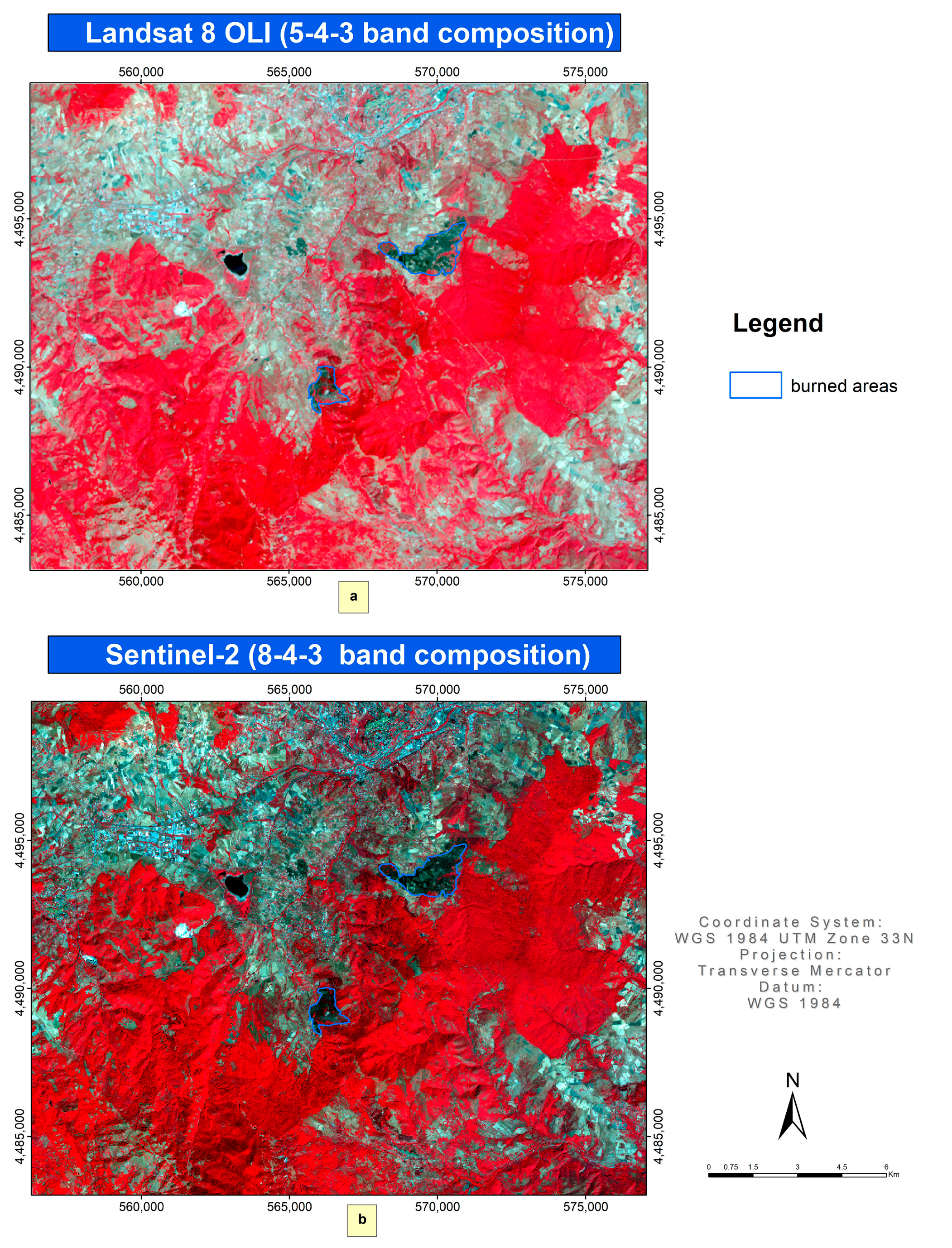
The burned areas were not present in the maps used, but a visual analysis of the satellite images in various compositions (especially near-infrared composition) highlighted the presence of burnt areas. The overlapping, in fact, reflected the burned areas of the Anti Incendio Boschivo (AIB) layer of the Basilicata region. Figure 3 confirms the presence of two wildfires that occurred on 9 August 2017 and 15 August 2017, respectively.
For each of the land use classes, several ground truths were selected and used both in the implementation phase of the classification algorithm (training site) and for the validation of the accuracy of the maps obtained (validation). In particular, the selected training sites amounted to 308, distributed almost in percentage according to the extent of the various classes of LULC.
For each of these training sites, whose LULC attribute was extracted from the land use map, the correctness of the attribution was first verified, for the forest types, using the forest map of the Basilicata region. In the extraction of the points from the polygons of the land use map, foresight was taken to select them at a distance of not less than 45 m from the boundary between one land use class and another, in such a way that the pixels of the images from the satellite belonged, as far as possible, to a pure class. Furthermore, the condition of a minimum distance between the points of 45 m meant that, for each pixel, only one ground truth could fall. Subsequently, for each of these points, they were verified by photointerpretation, overlapping the vector file of the training sites on the AGEA orthophoto from 2017 of the Basilicata region (with a resolution of 20 cm). Thus, the procedure allowed for the precise attribution of the training sites to the various land uses. Only for 19 of these points, there was ambiguity in the attribution to the LULC class. To identify the exact class of land use for these points, verification in the field via GPS was necessary. The same procedure was used for the ground truth points used in the validation phase. In this case, 165 control points were randomly selected and subjected to verification for the training sites. For 12 points, there were difficulties in assigning the land use class and therefore the survey in the field was carried out using GPS. It is a well-established practice to choose training sites from pre-existing land use maps [73], but these must be of high quality [74], and it is important, in any case, to verify, although the procedure can be expensive, the congruence of the training with the real land use. The sampling approaches, protocols, and designs for the collection of calibration and validation data have gradually matured over time [2,40,75], with particular emphasis on the type of application that these data are intended for, such as time series analysis [76] or studies on classification techniques [77]. However, the focal point remains the choice of a good number of training sites of excellent quality and a good sampling design, as unbalanced samples can lead to substantial errors [78], especially with spatial data of high geometric resolution. It has even been shown [61], by testing various types of classifiers, that the size and quality of the sample of training sites have a greater impact on the accuracy than the classification algorithms used. Moreover, the quality of the training sites themselves is more important in SVM than their number [79]. An old rule of thumb applies to ML classification according to which the number of training sites must be at least ten times the number of classes. Instead, for SVM classifications and machine learning in general, numerous studies have established that SVM requires, to obtain good results in terms of accuracy, a lower sample size [61,80], although this algorithm also requires good training quality in terms of correct attribution to the various classes [81]. Therefore, as previously mentioned, particular attention was paid to the selection of the ground truth and the correct identification of land use, which proved to be a crucial phase [82] for obtaining good-accuracy LULC maps. The solution adopted to avoid excessive reductions in the classification accuracy due to unbalanced training data, which in any case also negatively affects SVM [83], consisted of the choice of equalized stratified random sampling [63].

2.4. The Classification Algorithms

Two of the most widely used pixel-based classification algorithms [59], which generally provide better results in terms of accuracy, were tested: Maximum Likelihood Classifier (MLC) [14] and Support Vector Machine (SVM), a machine learning technique [59]. In addition to the careful choice of training sites, the appropriate choice of classification methods is also decisive for obtaining good-quality land use maps [84]. No post-processing procedures (e.g., filtering) were applied to the classifications obtained, to avoid the application of this type of procedure affecting the correctness of the comparison between classifiers [85]. The classifications shown in Table 3 were implemented and compared.
The “S2-MLC-with-RE” and “S2-SVM-with-RE” classifications provided for the implementation of the red-edge bands to verify the contribution of the same in improving the accuracy of the classification compared to “S2-MLC-without-RE” and “S2-SVM-without-RE”. Furthermore, “OLI-MLC” vs. “OLI-SVM”, “S2-MLC-without-RE” vs. “S2-SVM-without-RE”, and “S2-MLC-with-RE” vs. “S2-SVM-with-RE” provided information on the best-performing classification algorithm.
MLC represents one of the most used methods among the parametric classification approaches. In this type of approach, it is assumed that the data are distributed according to a predefined probability model and the parameters of this distribution depend on the input data of the training sites. In MLC, in particular, the unknown pixels are assigned to the specific class using the probability of the contours around the training area using the maximum likelihood approach. MLC requires a sufficient number of ground truths to be able to estimate the mean vector and the population variance/covariance matrix. The pixels are assigned to each class based on the threshold value provided by the user. If the probability value of the class is lower than the threshold value set by the user, the pixels are not classified [86]. In the case study, all the pixels were forced to belong to some class in such a way as not to have unclassified pixels. MLC is considered, among the supervised classifiers of the parametric type, the one that provides the best results [84]. Machine learning algorithms, typically non-parametric, do not make assumptions regarding the distribution of input data and are flexible and robust concerning the non-linear and noisy relationships between input characteristics and land use classes. Ultimately, these algorithms do not make assumptions about the normality of distribution and find more and more space in the remote sensing literature [59,87].
SVM is a widely used algorithm as it has high potential for complex and high-dimensional data, i.e., many predictive variables [61,79,88] and with unbalanced datasets [89,90]. The advantage of SVM is to provide good accuracy even with a rather small number of training sites [80,91]. The SVM algorithm [92] is a supervised machine learning classifier, trained for the optimal identification of the separation hyperplane, by maximizing the boundaries between classes [90]. The identified hyperplanes not only maximize the distance between the classes but are such that they do not include any points between them [61]. The points closest to the hyperplane are called support vectors [93]. For the identification of non-linearly separable classes, four kernel functions are often used in SVM: linear, polynomial, radial basis function (RBF), and sigmoid. RBF was chosen for this work due to its superiority as demonstrated in several studies (e.g., [14,61]). This function has two user-defined parameters that can affect the accuracy of the classification [94]: cost (C), a value used to adapt to classification errors in the training site dataset, and gamma (g), which influences the shape of the separation hyperplane:
K x i x j = e x p g x i x j 2
where K is the RB kernel, x i x j are two samples (feature vectors in some input space), and g is a free parameter. For a more correct comparison between images from different sources, the default values of the parameters were used in this work; in particular, for g, the default setting is given by the inverse of the number of calculated attributes. The default value of C is equal to 100. Among other aspects, according to Melgani and Bruzzone [95] and Maxwell et al. [63,96], the parameter optimization procedures may not lead to significantly different results in the accuracy of the classifications.
For the accuracy assessment of the classifications, one of the most commonly used approaches in classifications from satellite data was used: the error matrix [75]. The evaluation of accuracy is significant only when it is designed in a transparent and statistically defensible way. The resolution of the error matrix provides evaluation elements on Overall Accuracy (OA), User’s Accuracy (UA), Producer’s Accuracy (PA), Omission Error (OE), Commission Error (CO), and the Kappa coefficient [75,80,97,98,99].
An OE occurs when a pixel is assigned to the wrong class, while a CE arises when a pixel of another class is assigned to the class in question. The OE for each class, whose complement is called PA, is calculated as the ratio between the pixels of the main diagonal of the error matrix and the total pixels recognized as belonging to that particular class. Instead, the CE, whose complement is called UA, is defined as the ratio between the pixels on the diagonal and the sum of the row elements corresponding to a certain class. The OA of a confusion matrix is the ratio between the number of correctly classified pixels and the number of all ground truth pixels Nt:
O A = 1 N t i = 1 r n i
The Kappa coefficient is a measure of the overall agreement statistic of an error matrix and is recognized as a powerful method of measuring errors and comparing the differences between various error matrices [99]. Its formulation is as follows:
K = N i n m i , i 1 n ( G i C i )   N 2 1 n ( G i C i )
where i is the class number, n is the total number of classes, N is the total number of classified values compared to truth values, mi,i is the number of values belonging to the truth class i that has also been classified as class i, Gi is the total number of truth values belonging to class i, and Ci is the total number of predicted values belonging to class i.

3. Results

Preliminarily, as suggested by various authors [100], an analysis of the separability of training sites was conducted using the Jeffries–Matusita distance test (J–M). The value of J–M theoretically ranges from 0 to 2.0, and values above 1.8 indicate statistically good separability [101]. The data analysis showed good separability between the different land use categories for both Landsat 8 OLI and Sentinel-2 images, with values higher than 1.8. Only for some categories, the separability was not statistically significant (Table 4).
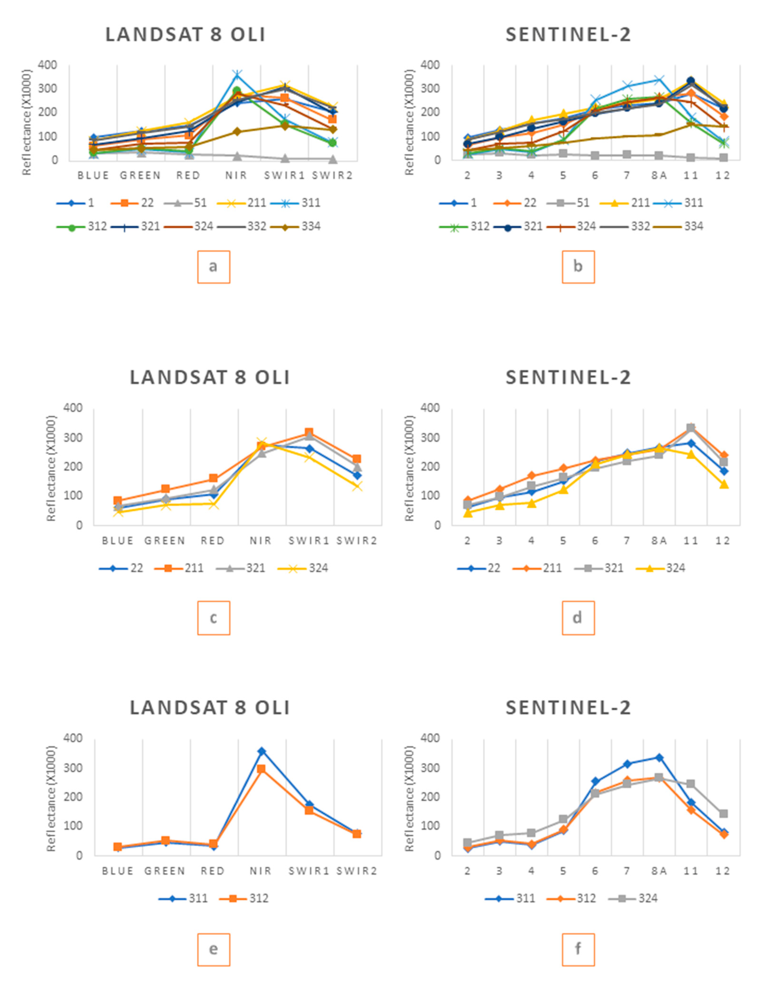
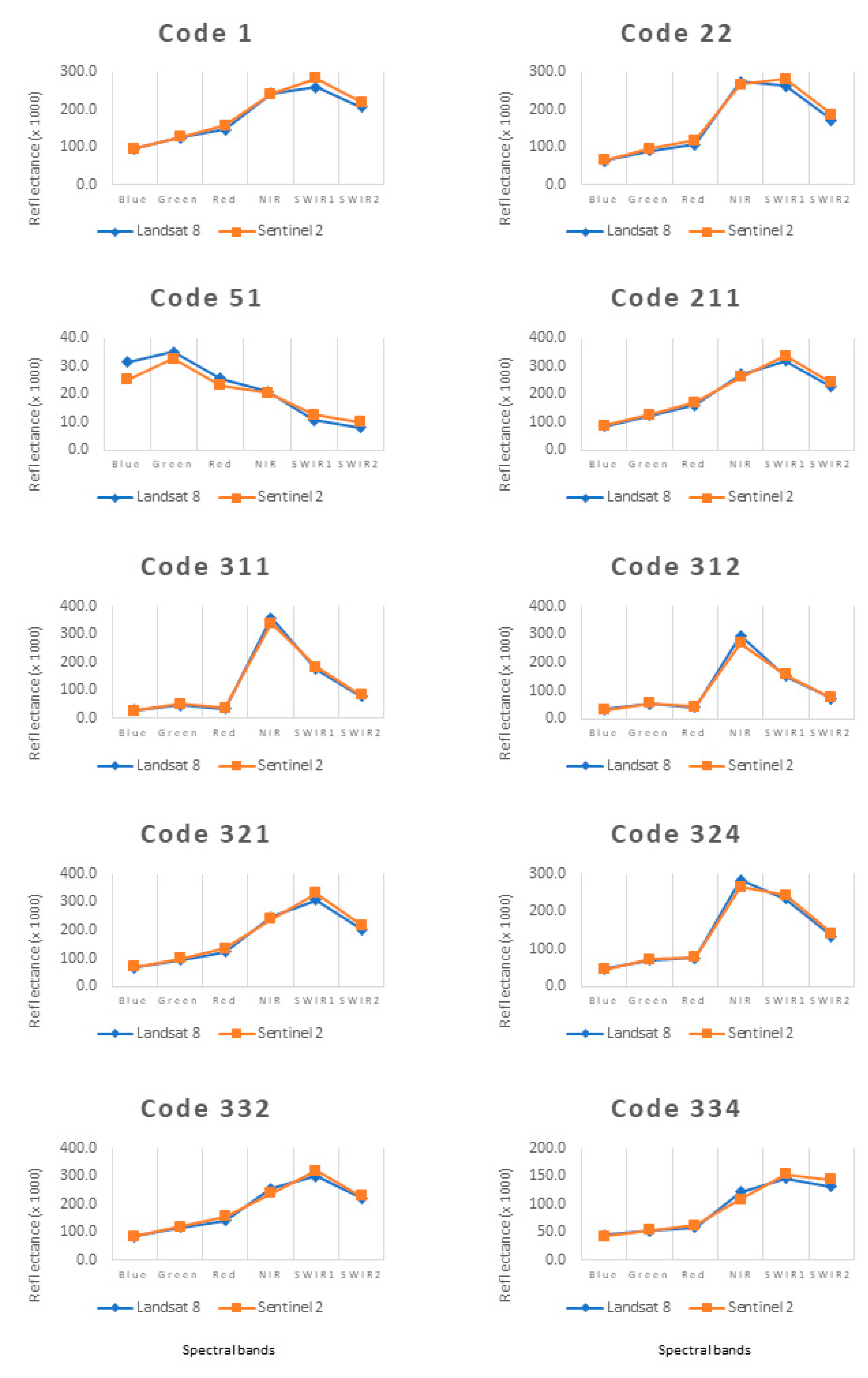
For both Landsat 8 and Sentinel-2, the most confused categories are arable crops (cereal crops) with natural grasslands. Analyzing the spectral trends (Figure 4c,d), it can be seen that the response of the two land use classes, both for Landsat 8 and Sentinel-2, basically follows the same trend, and the two curves are very slightly different. Among other aspects, analyzing the spectral responses of these two categories (Figure 5) for the two sensors, it is evident that there is very little difference, especially in the spectral range up to NIR; only for SWIR1 and SWIR2, there is a difference, albeit modest, between the two sensors, with Sentinel-2 reflectance values greater than those of Landsat 8 OLI.
A particularly confused category, both with Landsat 8 and Sentinel-2, is “Permanent crops”, which is not discriminable, especially from “Arable land” and, secondarily, “Transitional woodland-shrub” and “Natural grasslands” (Figure 4c,d). Finally, there is confusion, both for L8 and for S2, between the “Broad-leaved forests” and the “Coniferous forests” classes. Analyzing the spectral trends between the two sensors (Figure 4e,f), they are almost similar in the two categories. A greater distinction between conifers and broad-leaved trees is identified in the NIR region. Such differences are almost similar in OLI and MSI, with higher reflectance values in broad-leaved trees than in conifers. In general, however, by comparing the Landsat 8 and Sentinel-2 values for the two forest types (Figure 5), it can be seen how the trends overlap, with a slight difference in the NIR, where Sentinel shows slightly higher reflectance values than OLI. Finally, it should be noted that in S2, unlike L8, broad-leaved forests are confused not only with conifers but also with the “Transitional woodland-shrub” class (Figure 4f).
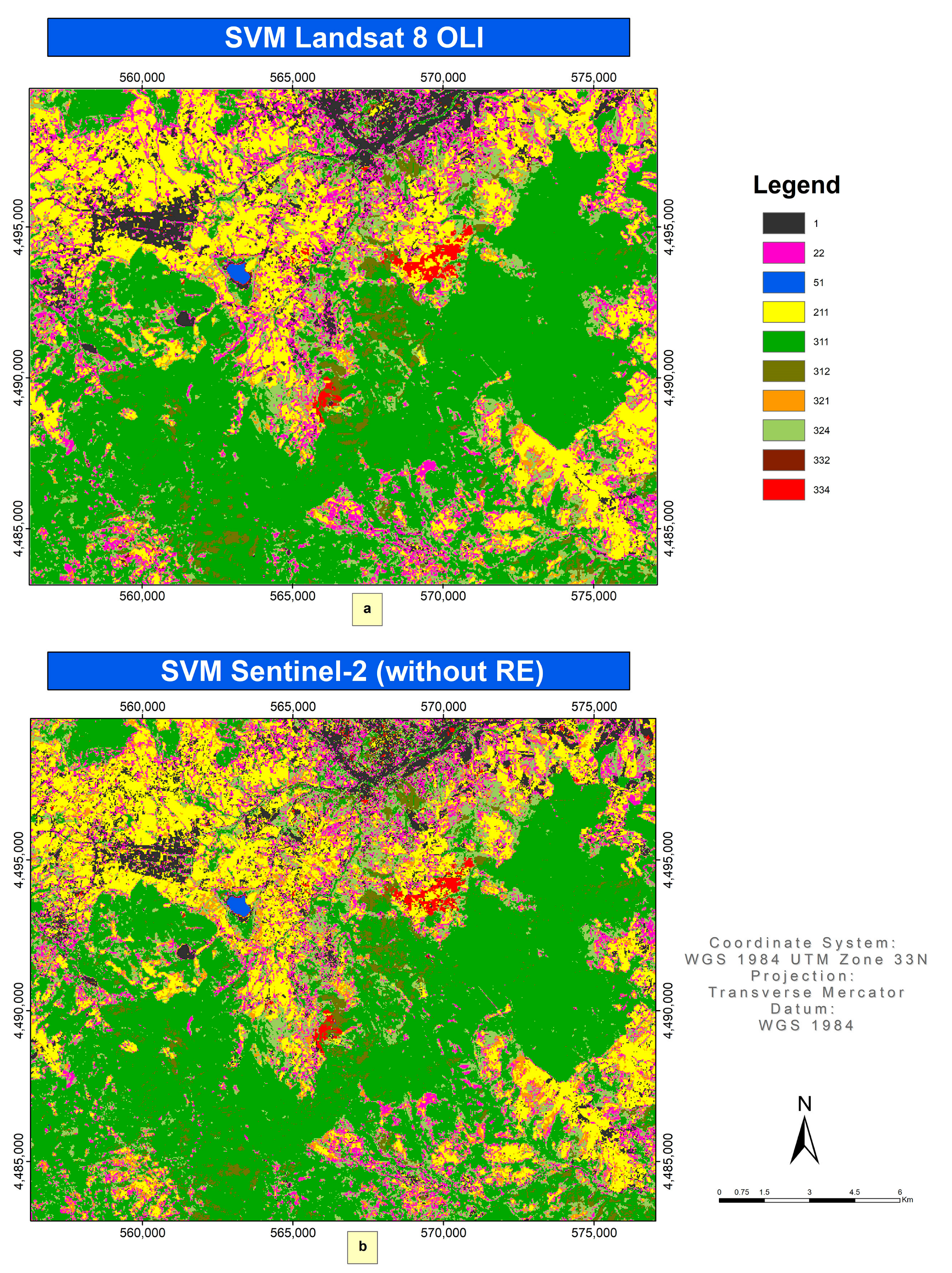
The results of all the classifications described above are reported in Figure 6, Figure 7 and Figure 8.
Analyzing the different land use classes for the different classifications, it is evident that the classifiers that show the least divergent area percentages with regard to the land use map of the Basilicata region (Table 2) are “OLI-MLC” and “OLI-SVM”, while the major differences are found with “S2-MLC-without-RE” and “S2-MLC-with-RE”. In the latter, the addition of the RE bands did not always lead to an improvement in the percentage differences, such as for “Broad-leaved forest”. The SVM classifier conducted on the S2 bands, with and without the RE bands, shows quite small differences in terms of areas. For all classifiers, the greatest percentage differences with respect to the reference map relate to the following two land use classes: “Permanent crops” and “Broad-leaved forest”. The “Permanent crops” are not very present in the study area, as they occupy an area of just over 1%, while all the classifiers report areas of around 10%. The minor deviations are provided by the classifiers that use the S2 bands, particularly by “S2-SVM-without-RE”, which presents minor differences, ~7%, compared to the reference map. Woody crops are often confused with deciduous trees, especially with forests undergoing natural expansion at their edges. The lower density of forest cover leads to confusion with tree crops (orchards, olive groves, and vineyards). Further, the percentage areas of “Broad-leaved forest” are underestimated, as all classifiers exhibit a percentage area around 40%, against ~50% of the reference map. Minor deviations, of ~6%, are reported by “OLI-SVM” and also the other SVM classifiers are better than the MLC classifications in terms of percentage areas. This is probably due to the well-known minor fragmentation of SVM classifications compared to MLC and to the choice not to apply, for a more correct comparison, any filter to the MLC classifications. Even the “Coniferous forests”, although not very present, are generally well discriminated, with deviations of 1–2% in all classifiers, especially those using the S2 bands. “OLI-MLC” also shows minor area differences (~1%) compared to the reference map for the categories “Transitional woodland-shrub” and, above all, “Natural grasslands”. In the latter case, the ability to discriminate, compared to the other classifiers, is significant: “OLI-MLC” overestimates by ~2%, while “OLI-SVM” underestimates by more than 5%. For this land use type, the situation is analogous with the classifiers using the S2 bands, i.e., smaller deviations of MLC compared to SVM, with slight improvements when also using the RE bands. The “Non-irrigated arable land”, which, according to the reference map, occupies an area of ~19%, is generally underestimated in the MLC classifications (differences of ~5–6%), while the differences with the SVM classifiers are very limited. This result is analogous to that of deciduous forests, i.e., the greater fragmentation of the MLC classifications, which manage to capture differences in cover within areas attributable to other land uses. Finally, all the classifiers show very small deviations for “Burnt areas” (0–0.1%), “Inland waters” (0.2–0.3%), and “Bare rocks” (0–2%). Moreover, the “Artificial surfaces“ are generally well distinguished, with a better discriminatory capacity for the S2 bands and the MLC classifiers. The addition of the RE bands leads to practically zero differences compared to the reference map.
To test the accuracy of the classifications, the confusion matrix and its synthetic indexes (UA, PA, OA, Kappa coefficient) were used. The analysis of OA and K (Table 5 and Figure 9) has shown that the classification that provides the best results in terms of accuracy is the MLC classification applied on Landsat 8 OLI data, which presents OA = 89%, and K = 0.87. The SVM classification with OLI data has lower accuracy values than MLC, with OA = 0.79 and therefore with a significant deterioration in performance.
Classifications made with Sentinel-2 data provide lower performance than Landsat 8 and, among these, the best performance is obtained for those that adopt MLC as a classification algorithm. MLC, in fact, with the S-2, without the red-edge bands, has an OA equal to 81.6% (for a K = 0.79), while the homologous one with SVM has accuracy of 72.3%, with a substantial difference in performance efficiency. MLC with Landsat compared to the corresponding classification (using the same bands) has a total accuracy level, compared to Sentinel-2, greater than approximately 8%. The worst results are provided by the SVM classifiers using the Sentinel-2 bands. The addition of the red-edge bands to the SVM classifier does not significantly improve the overall accuracy, recording an increase in OA of ~1%.
The MLC classifier, therefore, has the best performance with both Landsat and Sentinel-2 bands, with better performance using the Landsat bands than the homologous Sentinel-2 bands. For Sentinel-2, adding red-edge bands to the MLC classifier improves the accuracy by ~5%, testifying to the importance of these bands in the discrimination of certain vegetation types. The total accuracy of the “S2-MLC-with-RE” classifier is very close to that of the MLC classifier with Landsat bands, while showing the latter’s performance to be better, with an OA difference of just over 2%. By analyzing the confusion matrices of the various experiments in more detail, it can be seen that in the ML classifications (both with Landsat and Sentinel-2), the classes that are not confused (Producer’s Accuracy = 100%) are “Water bodies” (code 51), “Bare rocks” (code 332), and “Burnt areas”, which therefore have an excellent capacity for discrimination concerning other land use classes. The “OLI-MLC” classifier also performs well for other land uses (especially for all forest lands and “artificial surfaces”). The greatest confusion is for “Non-irrigated arable land”, with a PA = ~65%, confused above all with “Natural grasslands” (code 321) and, secondarily, with “Permanent crops” (code 22). As mentioned, the discrimination capacity of forest lands is very good, with accuracy generally higher than 95%. Only the “Broad-leaved forests” have lower accuracy (~90%) and are confused with the other forest categories, especially with the transitional woodland-shrub (code 324) and, secondarily, with conifers. The natural grasslands (code 321) also show good interpretative capacity (PA = ~97%) and are confused only with the burnt areas.
The homologous classification conducted using the Sentinel-2 bands (“S2-MLC-without-RE”) has, as mentioned, a total accuracy value lower than the previous one of ~ 8%. Moreover, in this case, the land use classes with a discriminatory capacity equal to 100% are the “Water bodies” (code 51), the “Bare rocks” (code 332), and the “Burnt areas” (code 334). “Non-irrigated arable land” (code 211) has the same level of accuracy as the homologous classification with Landsat 8, resulting, together with the “Permanent crops”, in the most confused class. The latter, compared to the “OLI-MLC” classifier, has an error of ~25% more and are confused above all with “Transitional woodland-shrub”, but also with non-irrigated arable land and bare rocks. The classifier also shows a substantial worsening for all forest categories compared to “OLI-MLC”. Only the “Broad-leaved forests” have almost comparable values, with differences of ~3%, while the other categories recorded substantial worsening. The “Coniferous Forests”, in particular, show levels of confusion of ~17% more than the previous classifier and are mainly confused with the “Transitional woodland-shrub” (code 324) and with the “Broad-leaved forests”. The discrimination capacity of “artificial surfaces” also worsens significantly (reduction in PA of around 8%).
The implementation of the red-edge bands in the MLC classification (“S2-MLC-with-RE”) leads to an increase in OA of ~5%. Moreover, in this case, the PA equal to 100% concerns bare soils, burnt areas, and water bodies. Compared to the MLC classification without the red-edge bands, the accuracy of all land use classes has improved, for the “Permanent crops” (code 22) in particular. The latter recorded an increase in accuracy equal to ~17% and are here confused only with arable land and shrubs, while in “S2-MLC-without”, they were confused with many other land use categories. The forest lands have also undergone an improvement in accuracy. Only the “Broad-leaved forests” have worsened slightly (reduction in accuracy of around 3%), confused with the “Transitional woodland-shrub”. The discrimination capacity of “Coniferous forests”, thanks to the inclusion of red edges, has increased considerably (~17%) and they are confused only with broad-leaved forests and no longer, as in “S2-MLC-without-RE”, even with shrubs. The natural grasslands show the same levels of accuracy, but, in this case, they are confused only with arable land and no longer also with bare rocks. The accuracy in identifying the “Transitional woodland-shrub” class has also improved (~3%), but, above all, the classes with which they are confused have been greatly reduced. In general, the introduction of red edges in the MLC classifier improves the OA and the accuracy of each class and significantly reduces the number of classes with which a given land use is confused. The SVM classifications all show worse performance than MLC and, among these, the one with the highest overall accuracy is the one conducted with Landsat data, although it shows a decrease in OA of ~14%. Many classes in “OLI-SVM” show a decrease in accuracy compared to “OLI-MLC”—in particular, the natural grasslands (code 321), the bare rocks (code 332), and the transitional woodland-shrub (code 324). Much improved, however, is the discrimination capacity of arable land (accuracy greater than approximately 20% compared to “OLI-MLC”), which is not confused with grasslands. Forest lands also show a better PA, albeit slightly, as they are less confused with conifers. SVM classifiers with Sentinel-2 bands have overall accuracy of just over 70%, nor does the inclusion of the red-edge bands in the classifier much improve the OA.

4. Discussion

Various studies have compared the performance of non-parametric classifiers, both with each other and in comparison with other parametric classifiers, in many territorial areas and for different types of classification ranging from agricultural to forestry areas to LULC [37,40,102], without reaching an unambiguous consensus on the performance of the various classification procedures. Several studies have compared the performance, of the same classifier, between spectral information deriving from different sensors and, in recent years, more specifically between data from the Landsat mission and the Copernicus Sentinel-2 data. Again, the studies do not reach an unambiguous consensus, attributing, in some cases, better performance to Landsat and, in others, to Sentinel data.
Most likely, this depends on several factors, including the characteristics of the study area, the type and quality of remote sensing data, the choice of LULC classes, and the selection of the related training sites. In the same in-depth review by Lu et al. [103], comparing different parametric and non-parametric classifiers, they conclude that the performance of the different classifiers depends on the datasets used. Some studies, in this regard, have shown how the addition of the Sentinel-2 red-edge bands to the various classifiers improves the discrimination capacity of the different land use classes, particularly of plant physiognomies and, above all, forest species. Some authors [28,104] have identified, with different classifiers, that the performance, using Landsat 8 and Sentinel-2, is very similar when using comparable bands between the two sensors, but that adding red edges to Sentinel data provides better results than Landsat.
Analyses conducted on classifications in Central Europe [55,101] have shown how the implementation of the red edge in classifiers can improve the discrimination capacity of forest stands. Previous studies [57,90] have highlighted the importance of red edges in distinguishing crops from the forest and that the entire dataset of Sentinel-2 bands leads to the discrimination of forest species [105,106] with levels of accuracy always very high, above 80%. Some authors [107] have highlighted, using Landsat 8, the importance of SWIR bands, together with NDVI, in the distinction of crops. The inclusion of NDVI in the classification, while it might be useful using OLI, would be redundant with Sentinel-2, where the radiometric input of the red-edge region is sufficient to improve the accuracy of the classification [28].
Immitzer et al. [17] demonstrated the good ability of Sentinel-2 to separate different land use classes, as well as to classify different forest types. The most important bands were SWIR, red, and NIR. The importance of NIR and SWIR for the classification of forest species has been highlighted among other aspects in other studies [17,101,105]. Immitzer et al. [17] conclude that the NIR band is the most important for the separation between conifers and broad-leaved forests, while the SWIR bands are more important for the identification of different forest species. Some authors [105] have identified that the narrower NIR band (8A), in Sentinel-2, is more important in the classification of the wider NIR band (band 8), and have highlighted the importance of red-edge bands in improving the classification accuracy.
Griffiths et al. [15], for the mapping of agricultural areas in Germany, using Landsat OLI and Sentinel-2 multitemporal data, obtained good results, with accuracy greater than 80%, demonstrating how the inclusion in the Random Forest (RF) classification processes of the red-edge bands lead to a slight improvement in overall performance, especially for classes concerning crops. For forests, numerous studies [78,108] have identified the importance of the visible and near-infrared bands in forest classification. Further studies [101] have highlighted the importance of the red-edge bands in the classification of various forest types. These studies highlight the remarkable potential of red-edge bands in forest classification compared to past multispectral sensors without these bands [109,110]. Of the red-edge bands, band 5 (705 nm) is important to distinguish various types of herbaceous crops [111], band 6 to better discriminate natural grasslands from herbaceous crops, and finally band 7 (783 nm) to better separate forest species. Korhonen et al. [52] identified that the red-edge bands, together with the SWIR bands, are the most significant for the discrimination of forest types in the boreal area. Similar results were also obtained by Persson et al. [105]. The importance of the SWIR bands (centered at 1610 nm and 2190 nm, band 11 and band 12, respectively) could be due to their ability to detect the variability of the water content of the different forest species and, therefore, to help discriminate them better [112]. As for the types of classifiers, also in this case, as mentioned, there is no agreement on which ones, with the same input data, provide better performance. SVM can provide, according to some authors [59], by its high ability to generalize complex characteristics, generally better results than parametric classifiers. Goodin et al. [113], using Landsat 8 data, identified overall accuracy of 88%, while Mansaray et al. [114] recorded, with SVM using Landsat 8 and Sentinel-1 and Sentinel-2, accuracy of 93.4%. Khatami et al. [38] found that SVM is the most efficient machine learning algorithm in many applications, outperforming RF, neural networks, and decision trees. Abdi [82] also identified, by comparing four non-parametric algorithms, the best performance of SVM compared to other machine learning classifiers. According to Adam et al. [90] and Li et al. [115], machine learning algorithms (SVM and RF in particular) provide comparable results in terms of accuracy, while Zhang and Xie [116] and Maxwell et al. [96,117] found SVM to perform better than RF. Gong et al. [118] and Yu et al. [119], comparing different parametric and non-parametric classifiers, come to the same conclusion, namely the better accuracy of the SVM classifications.
Furthermore, this classifier provides better performance through a pixel-based approach rather than an object-based one. The conclusions reached by other authors are the opposite: Nivedita Priyadarshini et al. [120], testing Sentinel-2 using different unsupervised and supervised classification algorithms (including MLC and SVM), have reported that MLC shows better performance in terms of accuracy, obtaining OA = 89.3% and OA = 75.6% for MLC and SVM, respectively. Nezhad M. et al. [121] also identified MLC’s performance is always higher than that of SVM in the classification of urban and periurban areas of the city of Rome using Sentinel-2 multitemporal images.
The present study always shows better results for MLC classifications than SVM, with differences, using Landsat 8 OLI images, of ~11%. Using the Sentinel-2 bands, without the red edges, the difference is ~10%. If we also input the red edges, the difference between MLC and SVM increases considerably (the MLC is better than SVM by ~15%), because, while, in MLC, the implementation of the red edge improves the accuracy, in SVM, it even worsens it, albeit slightly. The difference in accuracy between ML and SVM could also be because SVM does not use all the data from the training sample but only a subset that defines the boundary or margin conditions (support vector). This would suggest [63] that, in SVM, the strategy for collecting training sites should focus not on typical pixels but on pixels that could be spectrally confused with other classes. Furthermore, the quality of training sites plays a fundamental role in ML classifications—more so than their number—which, paradoxically, could lead to the well-known Hughes effect [122], i.e., a reduction in accuracy with increasing sample dimensionality.
The training sites were chosen, in the study site, with an almost balanced criterion, to take into account the percentage distribution of the different land use classes, and selected in such a way as to select pure pixels, and this could have influenced the greater accuracy of the MLC classifications versus the corresponding SVM ones. Finally, it must be said that the choice not to optimize the parameters of the tested classifiers, without, therefore, the iterative search for the best value of the parameters, could have affected the accuracy of the classification. The choice, however, was imposed by the need for a fair comparison between classifiers without introducing a priori knowledge [82]. In general, it can be said that the most confused classes, both among the classifiers taken into consideration and considering the data of the two different sensors, are between non-irrigated arable land (code 211) and natural grasslands (code 321), as already identified in previous studies [17]. Probably, the choice of a mono-temporal image is not able to fully distinguish between the various land use classes, particularly between crops and between these and natural grasslands. A careful choice that takes into account the phenology of the prevalent herbaceous crops could allow better discrimination of these with pastures. It is also possible that the optimal choice, depending on the land use classes present in the study area, of a single image, could allow for obtaining results very similar to multitemporal images throughout the year [123]. In the case in question, the images in August coincide with the wheat harvest, which has already taken place, whose plant residues can be radiometrically confused with the natural herbaceous vegetation. In this case, the choice of an image of June (or the beginning of July), when the wheat growth is at its maximum stage, would probably be able to better discriminate the two land use classes. Similarly, images acquired in spring would probably better differentiate forest species [55,105].
The image acquired in August, while allowing a very satisfactory distinction between forest classes (especially with ML), presents some confusion between conifers and broad-leaved trees. Probably, a spring image, when the broad-leaved trees are not in full growth, would allow a better distinction between the two forest categories [124]. Furthermore, topographic correction would also improve the separability between conifers and deciduous trees, allowing us to reduce the confusion between the deciduous trees on the slopes in shade with the conifers. Topographic correction can represent an important phase of pre-processing, especially in mountainous regions [84,125,126,127]. The inclusion of red edges with Sentinel-2 in the ML classifier improves the capacity for the discernment of forest categories, particularly of conifers and shrublands [52,57,105]. Forkuor et al. [111] even go so far as to conclude that the red-edge bands are the most important for LULC, providing very similar levels of accuracy to the entire Sentinel-2 dataset. Puletti et al. [101] identify, in the red edges acquired in the summer, the best ability to distinguish between conifers, broad-leaved trees, and mixed forests. Furthermore, broad-leaved forests tend to be confused with “transitional woodland-shrub”. This is believed to be related to the fact that the species referable to code 324, especially in an advanced successional stage, are always species referable to broad-leaved trees and therefore easily confused with “broad-leaved forests” (code 311). Ultimately, even greater accuracy results are to be expected using multitemporal data (seasonal images in various phenological stages) [17,28,84,128].

5. Conclusions

In this study, ML and SVM classifiers were compared using Landsat OLI and Sentinel-2 mono-temporal images (both acquired in August 2017) and testing both classifications that use comparable predictors (bands) between Landsat and Sentinel and classifications that consider also the Sentinel-2 red-edge bands among the predictive variables. Particular attention was paid to the selection of ground truth for both training and validation, this being a fundamental element, now widely recognized for obtaining good-quality classifications, and being more important also for the same classification algorithm. The results showed that ML classifications compared to SVM always provide higher levels of accuracy: with the OLI bands, we achieved accuracy of ~89%, while the SVM classification conducted with the same bands presents OA = ~78%. Then, the performance of the Landsat 8 OLI datasets and the Sentinel-2 ones always show the best efficiency for the Landsat data: the ML classifications on the datasets that use comparable bands between the two sensors show differences, in terms of total accuracy, of ~8%. Finally, it was verified that the contribution in the classifiers of the red-edge bands in the Sentinel-2 dataset improves, with ML, the accuracy by ~5%, with performance therefore very close (difference of ~2%) to that of the ML classification conducted with the Landsat bands.
Definitively, the study confirms the fact that there is no univocal consensus in the literature on the type of classifier to be used and on the type of image to be used. This depends on the land use classes taken into consideration, their spatial distribution, the number of predictors used, and the general characteristics of the study area. It is therefore important to try and test, through accuracy metrics, various types of classifiers (both machine learning and parametric) and various types of satellite images to produce the optimal result for the area of interest.

Author Contributions

Conceptualization, G.M.; methodology, G.M.; software, G.M. and A.F.; validation, G.M.; formal analysis, G.M.; investigation, G.M.; resources, M.L.T.; data curation, G.M. and A.F.; writing—original draft preparation, G.M.; writing—review and editing, G.M., A.F., M.L.T., and R.C.; visualization, G.M., A.F., and M.L.T.; supervision, G.M.; project administration and funding acquisition, M.L.T. and R.C. All authors have read and agreed to the published version of the manuscript.

Funding

The present work was a further result of the project “SPRINt” (2018-AMB-00120), financed by “Fondazione Con il Sud”. This research received no external funding.

Data Availability Statement

Not applicable.

Acknowledgments

We sincerely thank Maria Lucia Lucia for the careful reading of the manuscript and the valuable suggestions.

Conflicts of Interest

The authors declare no conflict of interest.

References

  1. Coppin, P.; Jonckheere, I.; Nackaerts, K.; Muys, B.; Lambin, E. Review ArticleDigital Change Detection Methods in Ecosystem Monitoring: A Review. Int. J. Remote Sens. 2004, 25, 1565–1596. [Google Scholar] [CrossRef]
  2. Hermosilla, T.; Wulder, M.A.; White, J.C.; Coops, N.C. Land Cover Classification in an Era of Big and Open Data: Optimizing Localized Implementation and Training Data Selection to Improve Mapping Outcomes. Remote Sens. Environ. 2022, 268, 112780. [Google Scholar] [CrossRef]
  3. van der Meer, F.D.; van der Werff, H.M.A.; van Ruitenbeek, F.J.A. Potential of ESA’s Sentinel-2 for Geological Applications. Remote Sens. Environ. 2014, 148, 124–133. [Google Scholar] [CrossRef]
  4. Ferrara, A.; Kosmas, C.; Salvati, L.; Padula, A.; Mancino, G.; Nolè, A. Updating the MEDALUS--ESA Framework for Worldwide Land Degradation and Desertification Assessment. Land Degrad. Dev. 2020, 31, 1593–1607. [Google Scholar] [CrossRef]
  5. Huang, W.; Ding, M.; Li, Z.; Zhuang, J.; Yang, J.; Li, X.; Meng, L.; Zhang, H.; Dong, Y. An Efficient User-Friendly Integration Tool for Landslide Susceptibility Mapping Based on Support Vector Machines: SVM-LSM Toolbox. Remote Sens. 2022, 14, 3408. [Google Scholar] [CrossRef]
  6. Stratoulias, D.; Balzter, H.; Sykioti, O.; Zlinszky, A.; Tóth, V. Evaluating Sentinel-2 for Lakeshore Habitat Mapping Based on Airborne Hyperspectral Data. Sensors 2015, 15, 22956–22969. [Google Scholar] [CrossRef] [Green Version]
  7. Hadjal, M.; Medina-Lopez, E.; Ren, J.; Gallego, A.; McKee, D. An Artificial Neural Network Algorithm to Retrieve Chlorophyll a for Northwest European Shelf Seas from Top of Atmosphere Ocean Colour Reflectance. Remote Sens. 2022, 14, 3353. [Google Scholar] [CrossRef]
  8. Tulbure, M.G.; Broich, M. Spatiotemporal Dynamic of Surface Water Bodies Using Landsat Time-Series Data from 1999 to 2011. ISPRS J. Photogramm. Remote Sens. 2013, 79, 44–52. [Google Scholar] [CrossRef]
  9. Hedley, J.; Roelfsema, C.; Koetz, B.; Phinn, S. Capability of the Sentinel 2 Mission for Tropical Coral Reef Mapping and Coral Bleaching Detection. Sentin. Missions—New Oppor. Sci. 2012, 120, 145–155. [Google Scholar] [CrossRef]
  10. Goldewijk, K.K. Estimating Global Land Use Change over the Past 300 Years: The HYDE Database. Glob. Biogeochem. Cycles 2001, 15, 417–433. [Google Scholar] [CrossRef]
  11. Pesaresi, M.; Corbane, C.; Julea, A.; Florczyk, A.; Syrris, V.; Soille, P. Assessment of the Added-Value of Sentinel-2 for Detecting Built-up Areas. Remote Sens. 2016, 8, 299. [Google Scholar] [CrossRef] [Green Version]
  12. Feddema, J.J.; Oleson, K.W.; Bonan, G.B.; Mearns, L.O.; Buja, L.E.; Meehl, G.A.; Washington, W.M. The Importance of Land-Cover Change in Simulating Future Climates. Science 2005, 310, 1674–1678. [Google Scholar] [CrossRef] [PubMed] [Green Version]
  13. Chen, S.; Xu, X.; Sun, K.; Dong, Y.; Yu, M.; Hu, Q.; Gong, J. New Archaeological Discoveries Based on Spatial Information Technology and Cultural Analysis: Taking the Study of the Spatial Relationship between Ancient Chinese Capitals and the Natural Environment as an Example. Remote Sens. 2022, 14, 3298. [Google Scholar] [CrossRef]
  14. Otukei, J.R.; Blaschke, T. Land Cover Change Assessment Using Decision Trees, Support Vector Machines and Maximum Likelihood Classification Algorithms. Int. J. Appl. Earth Obs. Geoinformation 2010, 12, S27–S31. [Google Scholar] [CrossRef]
  15. Griffiths, P.; Nendel, C.; Hostert, P. Intra-Annual Reflectance Composites from Sentinel-2 and Landsat for National-Scale Crop and Land Cover Mapping. Remote Sens. Environ. 2019, 220, 135–151. [Google Scholar] [CrossRef]
  16. Frampton, W.J.; Dash, J.; Watmough, G.; Milton, E.J. Evaluating the Capabilities of Sentinel-2 for Quantitative Estimation of Biophysical Variables in Vegetation. ISPRS J. Photogramm. Remote Sens. 2013, 82, 83–92. [Google Scholar] [CrossRef] [Green Version]
  17. Immitzer, M.; Neuwirth, M.; Böck, S.; Brenner, H.; Vuolo, F.; Atzberger, C. Optimal Input Features for Tree Species Classification in Central Europe Based on Multi-Temporal Sentinel-2 Data. Remote Sens. 2019, 11, 2599. [Google Scholar] [CrossRef] [Green Version]
  18. Kennedy, R.E.; Yang, Z.; Cohen, W.B.; Pfaff, E.; Braaten, J.; Nelson, P. Spatial and Temporal Patterns of Forest Disturbance and Regrowth within the Area of the Northwest Forest Plan. Remote Sens. Environ. 2012, 122, 117–133. [Google Scholar] [CrossRef]
  19. Sankey, T.; Donager, J.; McVay, J.; Sankey, J.B. UAV Lidar and Hyperspectral Fusion for Forest Monitoring in the Southwestern USA. Remote Sens. Environ. 2017, 195, 30–43. [Google Scholar] [CrossRef]
  20. Fassnacht, F.E.; Latifi, H.; Stereńczak, K.; Modzelewska, A.; Lefsky, M.; Waser, L.T.; Straub, C.; Ghosh, A. Review of Studies on Tree Species Classification from Remotely Sensed Data. Remote Sens. Environ. 2016, 186, 64–87. [Google Scholar] [CrossRef]
  21. Astola, H.; Häme, T.; Sirro, L.; Molinier, M.; Kilpi, J. Comparison of Sentinel-2 and Landsat 8 Imagery for Forest Variable Prediction in Boreal Region. Remote Sens. Environ. 2019, 223, 257–273. [Google Scholar] [CrossRef]
  22. Wittke, S.; Yu, X.; Karjalainen, M.; Hyyppä, J.; Puttonen, E. Comparison of Two-Dimensional Multitemporal Sentinel-2 Data with Three-Dimensional Remote Sensing Data Sources for Forest Inventory Parameter Estimation over a Boreal Forest. Int. J. Appl. Earth Obs. Geoinformation 2019, 76, 167–178. [Google Scholar] [CrossRef]
  23. Houghton, R.A.; House, J.I.; Pongratz, J.; van der Werf, G.R.; DeFries, R.S.; Hansen, M.C.; Le Quéré, C.; Ramankutty, N. Carbon Emissions from Land Use and Land-Cover Change. Biogeosciences 2012, 9, 5125–5142. [Google Scholar] [CrossRef] [Green Version]
  24. Karlson, M.; Ostwald, M.; Reese, H.; Sanou, J.; Tankoano, B.; Mattsson, E. Mapping Tree Canopy Cover and Aboveground Biomass in Sudano-Sahelian Woodlands Using Landsat 8 and Random Forest. Remote Sens. 2015, 7, 10017–10041. [Google Scholar] [CrossRef] [Green Version]
  25. Lin, S.; Li, J.; Liu, Q.; Li, L.; Zhao, J.; Yu, W. Evaluating the Effectiveness of Using Vegetation Indices Based on Red-Edge Reflectance from Sentinel-2 to Estimate Gross Primary Productivity. Remote Sens. 2019, 11, 1303. [Google Scholar] [CrossRef] [Green Version]
  26. Omruuzun, F.; Baskurt, D.O.; Daglayan, H.; Cetin, Y.Y. Utilizing Hyperspectral Remote Sensing Imagery for Afforestation Planning of Partially Covered Areas. In Proceedings of the Image and Signal Processing for Remote Sensing XXI; SPIE: Toulouse, France, 2015; Volume 9643, pp. 732–739. [Google Scholar]
  27. Filipponi, F. Exploitation of Sentinel-2 Time Series to Map Burned Areas at the National Level: A Case Study on the 2017 Italy Wildfires. Remote Sens. 2019, 11, 622. [Google Scholar] [CrossRef] [Green Version]
  28. Sothe, C.; Almeida, C.; Liesenberg, V.; Schimalski, M. Evaluating Sentinel-2 and Landsat-8 Data to Map Sucessional Forest Stages in a Subtropical Forest in Southern Brazil. Remote Sens. 2017, 9, 838. [Google Scholar] [CrossRef] [Green Version]
  29. Roteta, E.; Bastarrika, A.; Padilla, M.; Storm, T.; Chuvieco, E. Development of a Sentinel-2 Burned Area Algorithm: Generation of a Small Fire Database for Sub-Saharan Africa. Remote Sens. Environ. 2019, 222, 1–17. [Google Scholar] [CrossRef]
  30. Zarco-Tejada, P.J.; Hornero, A.; Beck, P.S.A.; Kattenborn, T.; Kempeneers, P.; Hernández-Clemente, R. Chlorophyll Content Estimation in an Open-Canopy Conifer Forest with Sentinel-2A and Hyperspectral Imagery in the Context of Forest Decline. Remote Sens. Environ. 2019, 223, 320–335. [Google Scholar] [CrossRef]
  31. Foley, J.A.; DeFries, R.; Asner, G.P.; Barford, C.; Bonan, G.; Carpenter, S.R.; Chapin, F.S.; Coe, M.T.; Daily, G.C.; Gibbs, H.K.; et al. Global Consequences of Land Use. Science 2005, 309, 570–574. [Google Scholar] [CrossRef]
  32. Roy, D.P.; Wulder, M.A.; Loveland, T.R.; Woodcock, C.E.; Allen, R.G.; Anderson, M.C.; Helder, D.; Irons, J.R.; Johnson, D.M.; Kennedy, R.; et al. Landsat-8: Science and Product Vision for Terrestrial Global Change Research. Remote Sens. Environ. 2014, 145, 154–172. [Google Scholar] [CrossRef] [Green Version]
  33. Xue, L.; Kappas, M.; Wyss, D.; Wang, C.; Putzenlechner, B.; Thi, N.P.; Chen, J. Assessment of Climate Change and Human Activities on Vegetation Development in Northeast China. Sensors 2022, 22, 2509. [Google Scholar] [CrossRef]
  34. Pettorelli, N.; Wegmann, M.; Skidmore, A.; Mücher, S.; Dawson, T.P.; Fernandez, M.; Lucas, R.; Schaepman, M.E.; Wang, T.; O’Connor, B.; et al. Framing the Concept of Satellite Remote Sensing Essential Biodiversity Variables: Challenges and Future Directions. Remote Sens. Ecol. Conserv. 2016, 2, 122–131. [Google Scholar] [CrossRef]
  35. Wulder, M.A.; White, J.C.; Goward, S.N.; Masek, J.G.; Irons, J.R.; Herold, M.; Cohen, W.B.; Loveland, T.R.; Woodcock, C.E. Landsat Continuity: Issues and Opportunities for Land Cover Monitoring. Remote Sens. Environ. 2008, 112, 955–969. [Google Scholar] [CrossRef]
  36. Nay, J.; Burchfield, E.; Gilligan, J. A Machine-Learning Approach to Forecasting Remotely Sensed Vegetation Health. Int. J. Remote Sens. 2018, 39, 1800–1816. [Google Scholar] [CrossRef]
  37. Li, M.; Ma, L.; Blaschke, T.; Cheng, L.; Tiede, D. A Systematic Comparison of Different Object-Based Classification Techniques Using High Spatial Resolution Imagery in Agricultural Environments. Int. J. Appl. Earth Obs. Geoinformation 2016, 49, 87–98. [Google Scholar] [CrossRef]
  38. Khatami, R.; Mountrakis, G.; Stehman, S.V. A Meta-Analysis of Remote Sensing Research on Supervised Pixel-Based Land-Cover Image Classification Processes: General Guidelines for Practitioners and Future Research. Remote Sens. Environ. 2016, 177, 89–100. [Google Scholar] [CrossRef] [Green Version]
  39. Wulder, M.A.; Masek, J.G.; Cohen, W.B.; Loveland, T.R.; Woodcock, C.E. Opening the Archive: How Free Data Has Enabled the Science and Monitoring Promise of Landsat. Remote Sens. Environ. 2012, 122, 2–10. [Google Scholar] [CrossRef]
  40. Wulder, M.A.; Coops, N.C.; Roy, D.P.; White, J.C.; Hermosilla, T. Land Cover 2.0. Int. J. Remote Sens. 2018, 39, 4254–4284. [Google Scholar] [CrossRef] [Green Version]
  41. Loveland, T.R.; Belward, A.S. The IGBP-DIS Global 1km Land Cover Data Set, DISCover: First Results. Int. J. Remote Sens. 1997, 18, 3289–3295. [Google Scholar] [CrossRef]
  42. Friedl, M.A.; Sulla-Menashe, D.; Tan, B.; Schneider, A.; Ramankutty, N.; Sibley, A.; Huang, X. MODIS Collection 5 Global Land Cover: Algorithm Refinements and Characterization of New Datasets. Remote Sens. Environ. 2010, 114, 168–182. [Google Scholar] [CrossRef]
  43. Cihlar, J. Land Cover Mapping of Large Areas from Satellites: Status and Research Priorities. Int. J. Remote Sens. 2000, 21, 1093–1114. [Google Scholar] [CrossRef]
  44. Fritz, S.; See, L.; Rembold, F. Comparison of Global and Regional Land Cover Maps with Statistical Information for the Agricultural Domain in Africa. Int. J. Remote Sens. 2010, 31, 2237–2256. [Google Scholar] [CrossRef]
  45. Li, J.; Roy, D. A Global Analysis of Sentinel-2A, Sentinel-2B and Landsat-8 Data Revisit Intervals and Implications for Terrestrial Monitoring. Remote Sens. 2017, 9, 902. [Google Scholar] [CrossRef] [Green Version]
  46. Woodcock, C.E.; Allen, R.; Anderson, M.; Belward, A.; Bindschadler, R.; Cohen, W.; Gao, F.; Goward, S.N.; Helder, D.; Helmer, E.; et al. Free Access to Landsat Imagery. Science 2008, 320, 1011. [Google Scholar] [CrossRef] [PubMed]
  47. Chen, J.; Chen, J.; Liao, A.; Cao, X.; Chen, L.; Chen, X.; He, C.; Han, G.; Peng, S.; Lu, M.; et al. Global Land Cover Mapping at 30m Resolution: A POK-Based Operational Approach. ISPRS J. Photogramm. Remote Sens. 2015, 103, 7–27. [Google Scholar] [CrossRef] [Green Version]
  48. Drusch, M.; Del Bello, U.; Carlier, S.; Colin, O.; Fernandez, V.; Gascon, F.; Hoersch, B.; Isola, C.; Laberinti, P.; Martimort, P.; et al. Sentinel-2: ESA’s Optical High-Resolution Mission for GMES Operational Services. Remote Sens. Environ. 2012, 120, 25–36. [Google Scholar] [CrossRef]
  49. Berger, M.; Moreno, J.; Johannessen, J.A.; Levelt, P.F.; Hanssen, R.F. ESA’s Sentinel Missions in Support of Earth System Science. Remote Sens. Environ. 2012, 120, 84–90. [Google Scholar] [CrossRef]
  50. Torres, R.; Snoeij, P.; Geudtner, D.; Bibby, D.; Davidson, M.; Attema, E.; Potin, P.; Rommen, B.; Floury, N.; Brown, M.; et al. GMES Sentinel-1 Mission. Remote Sens. Environ. 2012, 120, 9–24. [Google Scholar] [CrossRef]
  51. Sibanda, M.; Mutanga, O.; Rouget, M. Comparing the Spectral Settings of the New Generation Broad and Narrow Band Sensors in Estimating Biomass of Native Grasses Grown under Different Management Practices. GIScience Remote Sens. 2016, 53, 614–633. [Google Scholar] [CrossRef]
  52. Korhonen, L.; Hadi; Packalen, P.; Rautiainen, M. Comparison of Sentinel-2 and Landsat 8 in the Estimation of Boreal Forest Canopy Cover and Leaf Area Index. Remote Sens. Environ. 2017, 195, 259–274. [Google Scholar] [CrossRef]
  53. Filella, I.; Penuelas, J. The Red Edge Position and Shape as Indicators of Plant Chlorophyll Content, Biomass and Hydric Status. Int. J. Remote Sens. 1994, 15, 1459–1470. [Google Scholar] [CrossRef]
  54. Clevers, J.G.P.W.; Gitelson, A.A. Remote Estimation of Crop and Grass Chlorophyll and Nitrogen Content Using Red-Edge Bands on Sentinel-2 and -3. Int. J. Appl. Earth Obs. Geoinformation 2013, 23, 344–351. [Google Scholar] [CrossRef]
  55. Immitzer, M.; Vuolo, F.; Atzberger, C. First Experience with Sentinel-2 Data for Crop and Tree Species Classifications in Central Europe. Remote Sens. 2016, 8, 166. [Google Scholar] [CrossRef]
  56. Dotzler, S.; Hill, J.; Buddenbaum, H.; Stoffels, J. The Potential of EnMAP and Sentinel-2 Data for Detecting Drought Stress Phenomena in Deciduous Forest Communities. Remote Sens. 2015, 7, 14227–14258. [Google Scholar] [CrossRef] [Green Version]
  57. Schuster, C.; Förster, M.; Kleinschmit, B. Testing the Red Edge Channel for Improving Land-Use Classifications Based on High-Resolution Multi-Spectral Satellite Data. Int. J. Remote Sens. 2012, 33, 5583–5599. [Google Scholar] [CrossRef]
  58. Zarco-Tejada, P.J.; Miller, J.R. Land Cover Mapping at BOREAS Using Red Edge Spectral Parameters from CASI Imagery. J. Geophys. Res. Atmospheres 1999, 104, 27921–27933. [Google Scholar] [CrossRef]
  59. Mountrakis, G.; Im, J.; Ogole, C. Support Vector Machines in Remote Sensing: A Review. ISPRS J. Photogramm. Remote Sens. 2011, 66, 247–259. [Google Scholar] [CrossRef]
  60. Ishibuchi, H.; Nozaki, K.; Tanaka, H.; Hosaka, Y.; Matsuda, M. Empirical Study on Learning in Fuzzy Systems by Rice Taste Analysis. Fuzzy Sets Syst. 1994, 64, 129–144. [Google Scholar] [CrossRef]
  61. Huang, C.; Davis, L.S.; Townshend, J.R.G. An Assessment of Support Vector Machines for Land Cover Classification. Int. J. Remote Sens. 2002, 23, 725–749. [Google Scholar] [CrossRef]
  62. Alajlan, N.; Bazi, Y.; Melgani, F.; Yager, R.R. Fusion of Supervised and Unsupervised Learning for Improved Classification of Hyperspectral Images. Inf. Sci. 2012, 217, 39–55. [Google Scholar] [CrossRef]
  63. Maxwell, A.E.; Warner, T.A.; Fang, F. Implementation of Machine-Learning Classification in Remote Sensing: An Applied Review. Int. J. Remote Sens. 2018, 39, 2784–2817. [Google Scholar] [CrossRef] [Green Version]
  64. Zhu, Z.; Woodcock, C.E. Object-Based Cloud and Cloud Shadow Detection in Landsat Imagery. Remote Sens. Environ. 2012, 118, 83–94. [Google Scholar] [CrossRef]
  65. Zhu, Z.; Wang, S.; Woodcock, C.E. Improvement and Expansion of the Fmask Algorithm: Cloud, Cloud Shadow, and Snow Detection for Landsats 4–7, 8, and Sentinel 2 Images. Remote Sens. Environ. 2015, 159, 269–277. [Google Scholar] [CrossRef]
  66. Mayer, B.; Kylling, A. Technical Note: The LibRadtran Software Package for Radiative Transfer Calculations—Description and Examples of Use. Atmospheric Chem. Phys. 2005, 5, 1855–1877. [Google Scholar] [CrossRef] [Green Version]
  67. Vermote, E.F.; Tanre, D.; Deuze, J.L.; Herman, M.; Morcette, J.-J. Second Simulation of the Satellite Signal in the Solar Spectrum, 6S: An Overview. IEEE Trans. Geosci. Remote Sens. 1997, 35, 675–686. [Google Scholar] [CrossRef] [Green Version]
  68. Roy, D.P.; Kovalskyy, V.; Zhang, H.K.; Vermote, E.F.; Yan, L.; Kumar, S.S.; Egorov, A. Characterization of Landsat-7 to Landsat-8 Reflective Wavelength and Normalized Difference Vegetation Index Continuity. Remote Sens. Environ. 2016, 185, 57–70. [Google Scholar] [CrossRef] [Green Version]
  69. Storey, J.; Roy, D.P.; Masek, J.; Gascon, F.; Dwyer, J.; Choate, M. A Note on the Temporary Misregistration of Landsat-8 Operational Land Imager (OLI) and Sentinel-2 Multi Spectral Instrument (MSI) Imagery. Remote Sens. Environ. 2016, 186, 121–122. [Google Scholar] [CrossRef] [Green Version]
  70. Townshend, J.R.; Justice, C.O.; Gurney, C.; McManus, J. The Impact of Misregistration on Change Detection. IEEE Trans. Geosci. Remote Sens. 1992, 30, 1054–1060. [Google Scholar] [CrossRef] [Green Version]
  71. Claverie, M.; Ju, J.; Masek, J.G.; Dungan, J.L.; Vermote, E.F.; Roger, J.-C.; Skakun, S.V.; Justice, C. The Harmonized Landsat and Sentinel-2 Surface Reflectance Data Set. Remote Sens. Environ. 2018, 219, 145–161. [Google Scholar] [CrossRef]
  72. Mancino, G.; Nolè, A.; Ripullone, F.; Ferrara, A. Landsat TM Imagery and NDVI Differencing to Detect Vegetation Change: Assessing Natural Forest Expansion in Basilicata, Southern Italy. IForest—Biogeosciences For. 2014, 7, 75–84. [Google Scholar] [CrossRef] [Green Version]
  73. Wessels, K.J.; Van den Bergh, F.; Roy, D.P.; Salmon, B.P.; Steenkamp, K.C.; MacAlister, B.; Swanepoel, D.; Jewitt, D. Rapid Land Cover Map Updates Using Change Detection and Robust Random Forest Classifiers. Remote Sens. 2016, 8, 888. [Google Scholar] [CrossRef] [Green Version]
  74. Hermosilla, T.; Wulder, M.A.; White, J.C.; Coops, N.C.; Hobart, G.W. Disturbance-Informed Annual Land Cover Classification Maps of Canada’s Forested Ecosystems for a 29-Year Landsat Time Series. Can. J. Remote Sens. 2018, 44, 67–87. [Google Scholar] [CrossRef]
  75. Foody, G.M. Status of Land Cover Classification Accuracy Assessment. Remote Sens. Environ. 2002, 80, 185–201. [Google Scholar] [CrossRef]
  76. Pelletier, C.; Valero, S.; Inglada, J.; Champion, N.; Marais Sicre, C.; Dedieu, G. Effect of Training Class Label Noise on Classification Performances for Land Cover Mapping with Satellite Image Time Series. Remote Sens. 2017, 9, 173. [Google Scholar] [CrossRef] [Green Version]
  77. Millard, K.; Richardson, M. On the Importance of Training Data Sample Selection in Random Forest Image Classification: A Case Study in Peatland Ecosystem Mapping. Remote Sens. 2015, 7, 8489–8515. [Google Scholar] [CrossRef] [Green Version]
  78. Immitzer, M.; Atzberger, C.; Koukal, T. Tree Species Classification with Random Forest Using Very High Spatial Resolution 8-Band WorldView-2 Satellite Data. Remote Sens. 2012, 4, 2661–2693. [Google Scholar] [CrossRef] [Green Version]
  79. Su, L.; Huang, Y. Support Vector Machine (SVM) Classification: Comparison of Linkage Techniques Using a Clustering-Based Method for Training Data Selection. GIScience Remote Sens. 2009, 46, 411–423. [Google Scholar] [CrossRef]
  80. Foody, G.M.; Mathur, A. A Relative Evaluation of Multiclass Image Classification by Support Vector Machines. IEEE Trans. Geosci. Remote Sens. 2004, 42, 1335–1343. [Google Scholar] [CrossRef] [Green Version]
  81. Foody, G.; Pal, M.; Rocchini, D.; Garzon-Lopez, C.; Bastin, L. The Sensitivity of Mapping Methods to Reference Data Quality: Training Supervised Image Classifications with Imperfect Reference Data. ISPRS Int. J. Geo-Inf. 2016, 5, 199. [Google Scholar] [CrossRef]
  82. Abdi, A.M. Land Cover and Land Use Classification Performance of Machine Learning Algorithms in a Boreal Landscape Using Sentinel-2 Data. GIScience Remote Sens. 2020, 57, 1–20. [Google Scholar] [CrossRef] [Green Version]
  83. Stumpf, A.; Kerle, N. Object-Oriented Mapping of Landslides Using Random Forests. Remote Sens. Environ. 2011, 115, 2564–2577. [Google Scholar] [CrossRef]
  84. Lu, D.; Weng, Q. A Survey of Image Classification Methods and Techniques for Improving Classification Performance. Int. J. Remote Sens. 2007, 28, 823–870. [Google Scholar] [CrossRef]
  85. Phiri, D.; Morgenroth, J. Developments in Landsat Land Cover Classification Methods: A Review. Remote Sens. 2017, 9, 967. [Google Scholar] [CrossRef] [Green Version]
  86. Ahmad, A.; Quegan, S. Analysis of Maximum Likelihood Classification Technique on Landsat 5 TM Satellite Data of Tropical Land Covers. In Proceedings of the 2012 IEEE International Conference on Control System, Computing and Engineering, Penang, Penang, Malaysia, 23 November 2012; pp. 280–285. [Google Scholar]
  87. Belgiu, M.; Drăguţ, L. Random Forest in Remote Sensing: A Review of Applications and Future Directions. ISPRS J. Photogramm. Remote Sens. 2016, 114, 24–31. [Google Scholar] [CrossRef]
  88. Pal, M.; Mather, P.M. Support Vector Machines for Classification in Remote Sensing. Int. J. Remote Sens. 2005, 26, 1007–1011. [Google Scholar] [CrossRef]
  89. Ham, J.; Chen, Y.; Crawford, M.M.; Ghosh, J. Investigation of the Random Forest Framework for Classification of Hyperspectral Data. IEEE Trans. Geosci. Remote Sens. 2005, 43, 492–501. [Google Scholar] [CrossRef] [Green Version]
  90. Adam, E.; Mutanga, O.; Odindi, J.; Abdel-Rahman, E.M. Land-Use/Cover Classification in a Heterogeneous Coastal Landscape Using RapidEye Imagery: Evaluating the Performance of Random Forest and Support Vector Machines Classifiers. Int. J. Remote Sens. 2014, 35, 3440–3458. [Google Scholar] [CrossRef]
  91. Foody, G.M.; Mathur, A.; Sanchez-Hernandez, C.; Boyd, D.S. Training Set Size Requirements for the Classification of a Specific Class. Remote Sens. Environ. 2006, 104, 1–14. [Google Scholar] [CrossRef]
  92. Cortes, C.; Vapnik, V. Support-Vector Networks. Mach. Learn. 1995, 20, 273–297. [Google Scholar] [CrossRef]
  93. Yuan, T.; Lee, H.; Jung, H.C.; Aierken, A.; Beighley, E.; Alsdorf, D.E.; Tshimanga, R.M.; Kim, D. Absolute Water Storages in the Congo River Floodplains from Integration of InSAR and Satellite Radar Altimetry. Remote Sens. Environ. 2017, 201, 57–72. [Google Scholar] [CrossRef]
  94. Burges, C.J.C. A Tutorial on Support Vector Machines for Pattern Recognition. Data Min. Knowl. Discov. 1998, 2, 121–167. [Google Scholar] [CrossRef]
  95. Melgani, F.; Bruzzone, L. Classification of Hyperspectral Remote Sensing Images with Support Vector Machines. IEEE Trans. Geosci. Remote Sens. 2004, 42, 1778–1790. [Google Scholar] [CrossRef] [Green Version]
  96. Maxwell, A.E.; Strager, M.P.; Warner, T.A.; Zégre, N.P.; Yuill, C.B. Comparison of NAIP Orthophotography and RapidEye Satellite Imagery for Mapping of Mining and Mine Reclamation. GIScience Remote Sens. 2014, 51, 301–320. [Google Scholar] [CrossRef]
  97. Congalton, R.G. Assessing Landsat Classification Accuracy Using Discrete Multivariate Analysis Statistical Techniques. Photogramm. Eng. Remote Sens. 1983, 49, 1671–1678. [Google Scholar]
  98. Hudson, W.D.; Ramm, C.W. Correct Formulation of the Kappa Coefficient of Agreement. Photogramm. Eng. Remote Sens. 1987, 53, 421–422. [Google Scholar]
  99. Congalton, R.G. A Review of Assessing the Accuracy of Classifications of Remotely Sensed Data. Remote Sens. Environ. 1991, 37, 35–46. [Google Scholar] [CrossRef]
  100. Vaglio Laurin, G.; Puletti, N.; Hawthorne, W.; Liesenberg, V.; Corona, P.; Papale, D.; Chen, Q.; Valentini, R. Discrimination of Tropical Forest Types, Dominant Species, and Mapping of Functional Guilds by Hyperspectral and Simulated Multispectral Sentinel-2 Data. Remote Sens. Environ. 2016, 176, 163–176. [Google Scholar] [CrossRef] [Green Version]
  101. Puletti, N.; Chianucci, F.; Castaldi, C. Use of Sentinel-2 for Forest Classification in Mediterranean Environments. Ann. Silvic. Res. 2018, 42, 32–38. [Google Scholar] [CrossRef]
  102. Dalponte, M.; Bruzzone, L.; Gianelle, D. Tree Species Classification in the Southern Alps Based on the Fusion of Very High Geometrical Resolution Multispectral/Hyperspectral Images and LiDAR Data. Remote Sens. Environ. 2012, 123, 258–270. [Google Scholar] [CrossRef]
  103. Lu, D.; Li, G.; Moran, E.; Kuang, W. A Comparative Analysis of Approaches for Successional Vegetation Classification in the Brazilian Amazon. GIScience Remote Sens. 2014, 51, 695–709. [Google Scholar] [CrossRef]
  104. Topaloğlu, R.H.; Sertel, E.; Musaoğlu, N. Assessment of Classification Accuracies of Sentinel-2 and Landsat-8 Data for Land Cover/Use Mapping. In Proceedings of the The International Archives of the Photogrammetry, Remote Sensing and Spatial Information Sciences; Copernicus GmbH: Prague, Czech Republic, 2016; Volume XLI-B8, pp. 1055–1059. [Google Scholar]
  105. Persson, M.; Lindberg, E.; Reese, H. Tree Species Classification with Multi-Temporal Sentinel-2 Data. Remote Sens. 2018, 10, 1794. [Google Scholar] [CrossRef]
  106. Grabska, E.; Hostert, P.; Pflugmacher, D.; Ostapowicz, K. Forest Stand Species Mapping Using the Sentinel-2 Time Series. Remote Sens. 2019, 11, 1197. [Google Scholar] [CrossRef] [Green Version]
  107. Schultz, B.; Immitzer, M.; Formaggio, A.R.; Sanches, I.D.A.; Luiz, A.J.B.; Atzberger, C. Self-Guided Segmentation and Classification of Multi-Temporal Landsat 8 Images for Crop Type Mapping in Southeastern Brazil. Remote Sens. 2015, 7, 14482–14508. [Google Scholar] [CrossRef] [Green Version]
  108. Waser, L.T.; Küchler, M.; Jütte, K.; Stampfer, T. Evaluating the Potential of WorldView-2 Data to Classify Tree Species and Different Levels of Ash Mortality. Remote Sens. 2014, 6, 4515–4545. [Google Scholar] [CrossRef] [Green Version]
  109. Sellers, P.J. Canopy Reflectance, Photosynthesis and Transpiration. Int. J. Remote Sens. 1985, 6, 1335–1372. [Google Scholar] [CrossRef] [Green Version]
  110. Thenkabail, P.S.; Smith, R.B.; De Pauw, E. Hyperspectral Vegetation Indices and Their Relationships with Agricultural Crop Characteristics. Remote Sens. Environ. 2000, 71, 158–182. [Google Scholar] [CrossRef]
  111. Forkuor, G.; Dimobe, K.; Serme, I.; Tondoh, J.E. Landsat-8 vs. Sentinel-2: Examining the Added Value of Sentinel-2′s Red-Edge Bands to Land-Use and Land-Cover Mapping in Burkina Faso. GIScience Remote Sens. 2018, 55, 331–354. [Google Scholar] [CrossRef]
  112. Lukeš, P.; Stenberg, P.; Rautiainen, M.; Mõttus, M.; Vanhatalo, K.M. Optical Properties of Leaves and Needles for Boreal Tree Species in Europe. Remote Sens. Lett. 2013, 4, 667–676. [Google Scholar] [CrossRef]
  113. Goodin, D.G.; Anibas, K.L.; Bezymennyi, M. Mapping Land Cover and Land Use from Object-Based Classification: An Example from a Complex Agricultural Landscape. Int. J. Remote Sens. 2015, 36, 4702–4723. [Google Scholar] [CrossRef]
  114. Mansaray, L.R.; Wang, F.; Huang, J.; Yang, L.; Kanu, A.S. Accuracies of Support Vector Machine and Random Forest in Rice Mapping with Sentinel-1A, Landsat-8 and Sentinel-2A Datasets. Geocarto Int. 2020, 35, 1088–1108. [Google Scholar] [CrossRef]
  115. Li, M.; Im, J.; Beier, C. Machine Learning Approaches for Forest Classification and Change Analysis Using Multi-Temporal Landsat TM Images over Huntington Wildlife Forest. GIScience Remote Sens. 2013, 50, 361–384. [Google Scholar] [CrossRef]
  116. Zhang, C.; Xie, Z. Object-Based Vegetation Mapping in the Kissimmee River Watershed Using HyMap Data and Machine Learning Techniques. Wetlands 2013, 33, 233–244. [Google Scholar] [CrossRef]
  117. Maxwell, A.E.; Warner, T.A.; Strager, M.P.; Conley, J.F.; Sharp, A.L. Assessing Machine-Learning Algorithms and Image- and Lidar-Derived Variables for GEOBIA Classification of Mining and Mine Reclamation. Int. J. Remote Sens. 2015, 36, 954–978. [Google Scholar] [CrossRef]
  118. Gong, P.; Wang, J.; Yu, L.; Zhao, Y.; Zhao, Y.; Liang, L.; Niu, Z.; Huang, X.; Fu, H.; Liu, S.; et al. Finer Resolution Observation and Monitoring of Global Land Cover: First Mapping Results with Landsat TM and ETM+ Data. Int. J. Remote Sens. 2013, 34, 2607–2654. [Google Scholar] [CrossRef] [Green Version]
  119. Yu, L.; Liang, L.; Wang, J.; Zhao, Y.; Cheng, Q.; Hu, L.; Liu, S.; Yu, L.; Wang, X.; Zhu, P.; et al. Meta-Discoveries from a Synthesis of Satellite-Based Land-Cover Mapping Research. Int. J. Remote Sens. 2014, 35, 4573–4588. [Google Scholar] [CrossRef]
  120. Nivedita Priyadarshini, K.; Kumar, M.; Rahaman, S.A.; Nitheshnirmal, S. A Comparative Study of Advanced Land Use/Land Cover Classification Algorithms Using Sentinel-2 Data. Int. Arch. Photogramm. Remote Sens. Spat. Inf. Sci. 2018, XLII–5, 665–670. [Google Scholar] [CrossRef] [Green Version]
  121. Nezhad, M.M.; Heydari, A.; Fusilli, L.; Laneve, G. Land Cover Classification by Using Sentinel-2 Images: A Case Study in the City of Rome. In Proceedings of the the 4th World Congress on Civil, Structural, and Environmental Engineering, Rome, Italy, 1 April 2019. [Google Scholar]
  122. Hughes, G. On the Mean Accuracy of Statistical Pattern Recognizers. IEEE Trans. Inf. Theory 1968, 14, 55–63. [Google Scholar] [CrossRef] [Green Version]
  123. Feilhauer, H.; Thonfeld, F.; Faude, U.; He, K.S.; Rocchini, D.; Schmidtlein, S. Assessing Floristic Composition with Multispectral Sensors—A Comparison Based on Monotemporal and Multiseasonal Field Spectra. Int. J. Appl. Earth Obs. Geoinformation 2013, 21, 218–229. [Google Scholar] [CrossRef]
  124. Murthy, C.S.; Raju, P.V.; Badrinath, K.V.S. Classification of Wheat Crop with Multi-Temporal Images: Performance of Maximum Likelihood and Artificial Neural Networks. Int. J. Remote Sens. 2003, 24, 4871–4890. [Google Scholar] [CrossRef]
  125. Teillet, P.M.; Guindon, B.; Goodenough, D.G. On the Slope-Aspect Correction of Multispectral Scanner Data. Can. J. Remote Sens. 1982, 8, 84–106. [Google Scholar] [CrossRef] [Green Version]
  126. Richter, R. Correction of Atmospheric and Topographic Effects for High Spatial Resolution Satellite Imagery. Int. J. Remote Sens. 1997, 18, 1099–1111. [Google Scholar] [CrossRef]
  127. Hale, S.R.; Rock, B.N. Impact of Topographic Normalization on Land-Cover Classification Accuracy. Photogramm. Eng. Remote Sens. 2003, 69, 785–791. [Google Scholar] [CrossRef] [Green Version]
  128. Pasquarella, V.J.; Holden, C.E.; Woodcock, C.E. Improved Mapping of Forest Typfe Using Spectral-Temporal Landsat Features. Remote Sens. Environ. 2018, 210, 193–207. [Google Scholar] [CrossRef]
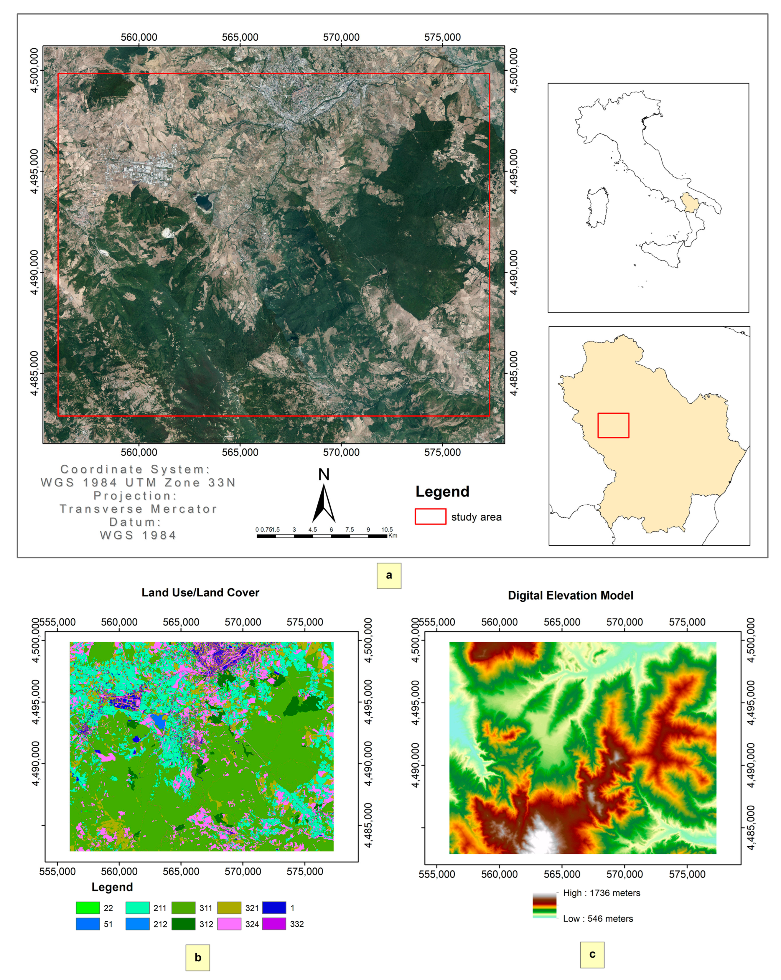
Figure 1. Maps of the study area: (a) Overview, (b) Land Use/Land Cover (class description: 1—Artificial surface, 22—Permanent crops, 51—Inland waters, 211—Non-irrigated arable land, 311—Broad-leaved forest, 312—Coniferous forest, 321—Natural grasslands, 324—Transitional woodland-shrub, 332—Bare rocks, 334—Burnt areas), (c) Digital Elevation Model.
Geographies 03 00005 g001
Figure 2. Sentinel-2 tile (in true color composition) overlapping the Landsat 8 OLI scene (in near-infrared composition).
Geographies 03 00005 g002
Figure 3. Burned areas overlapping (a) Landsat 8 (5-4-3) and (b) Sentinel-2 (8-4-3) false color composites covering the study area.
Geographies 03 00005 g003
Figure 4. Landsat 8 OLI and Sentinel-2 reflectance values ((a,b) for all and (cf) for some significant land use classes).
Geographies 03 00005 g004
Figure 5. Differences between the reflectance values, for different land use classes, between Landsat 8 OLI and Sentinel-2.
Geographies 03 00005 g005
Figure 6. MLC classifications with (a) Landsat 8 OLI and with (b) Sentinel-2 without red-edge bands.
Geographies 03 00005 g006
Figure 7. SVM classifications with (a) Landsat 8 OLI and with (b) Sentinel-2 without red-edge bands.
Geographies 03 00005 g007
Figure 8. (a) MLC and (b) SVM classifications with Sentinel-2 including red-edge bands.
Geographies 03 00005 g008
Figure 9. Accuracy (OA and K) for the different classifications tested.
Geographies 03 00005 g009
Table 1. Spectral bands of Landsat 8 OLI and Sentinel-2 MSI that were used for the comparison of classification algorithms.
Landsat 8 OLISentinel-2 MSI
BandWavelength
Range (nm)
Resolution (m)BandWavelength
Range (nm)
Resolution (m)
B2 (Blue)452.0–512.030B2459.4–525.410
B3 (Green)533.0–590.030B3541.8–577.810
B4 (Red)636.0–673.030B4649.1–680.110
B5 (NIR)851.0–879.030B8A852.2–875.220
B6 (SWIR 1)1566.0–1651.030B111568.2–1659.220
B7 (SWIR 2)2017.0–2294.030B122114.9–2289.920
B5 (Red-Edge)696.6–711.620
B6 (Red-Edge)733.0–748.020
B7 (Red-Edge)772.8–792.820
Table 2. Absolute and percentage area of LULC classes in the study area.
CodeDescriptionArea (ha)Area (%)
1Artificial surface18625.1
22Permanent crops4671.3
51Inland waters1250.3
211Non-irrigated arable land685418.9
311Broad-leaved forest18,42650.9
312Coniferous forest9962.8
321Natural grasslands27977.7
324Transitional woodland-shrub444612.3
332Bare rocks30.0
334Burnt areas2080.6
Total36,184100.0
Table 3. Classifications, algorithms, sensors, and bands used for the comparison tests.
ClassificationAlgorithmSensorBands Used
OLI-MLCMaximum Likelihood ClassifierLandsat 8 OLI2, 3, 4, 5, 6, 7
OLI-SVMSupport Vector MachineLandsat 8 OLI2, 3, 4, 5, 6, 7
S2-MLC-without-REMaximum Likelihood ClassifierSentinel-2 MSI2, 3, 4, 8A, 11, 12
S2-MLC-with-REMaximum Likelihood ClassifierSentinel-2 MSI2, 3, 4, 5, 6, 7, 8A, 11, 12
S2-SVM-without-RESupport Vector MachineSentinel-2 MSI2, 3, 4, 8A, 11, 12
S2-SVM-with-RESupport Vector MachineSentinel-2 MSI2, 3, 4, 5, 6, 7, 8A, 11, 12
Table 4. Jeffries–Matusita (J–M) distance values for the two sensors examined and for confused LULC classes.
Landsat 8 OLISentinel-2 MSI
ComparisonJ–M ValueComparisonJ–M Value
211 vs. 3211.4359211 vs. 3211.4611
22 vs. 2111.599522 vs. 2111.5570
311 vs. 3121.635322 vs. 3241.5951
22 vs. 3241.6379311 vs.3121.6440
22 vs. 3211.670122 vs. 3211.7678
311 vs. 3241.7960
Table 5. Classifications’ accuracy assessment.
Producer’s AccuracyUser’s Accuracy
LULC ClassesLULC Classes
Classification1225121131131232132433233412251211311312321324332334OA (%)K
OLI-MLC90.489.7100.065.289.695.795.897.0100.0100.097.981.3100.093.898.491.769.784.268.893.389.030.8745
OLI-SVM86.551.7100.084.891.065.229.275.845.585.780.460.0100.059.188.483.3100.062.5100.092.378.510.7183
S2-MLC-without-RE82.765.5100.065.286.678.391.781.8100.0100.0100.065.5100.083.395.172.068.873.052.493.381.610.7900
S2-MLC-with-RE86.582.8100.078.383.695.791.784.9100.0100.0100.077.4100.081.896.671.073.382.491.7100.086.770.8486
S2-SVM-without-RE80.862.1100.080.489.665.229.269.70.078.676.464.3100.054.484.575.070.065.70.091.772.260.6765
S2-SVM-with-RE80.862.1100.080.489.665.229.269.70.078.678.265.4100.052.882.276.580.062.2100.092.371.610.6683
Disclaimer/Publisher’s Note: The statements, opinions and data contained in all publications are solely those of the individual author(s) and contributor(s) and not of MDPI and/or the editor(s). MDPI and/or the editor(s) disclaim responsibility for any injury to people or property resulting from any ideas, methods, instructions or products referred to in the content.