

On the Use of MATLAB to Import and Manipulate Geographic Data: A Tool for Landslide Susceptibility Assessment

Abstract
:1. Introduction
2. Materials and Methods
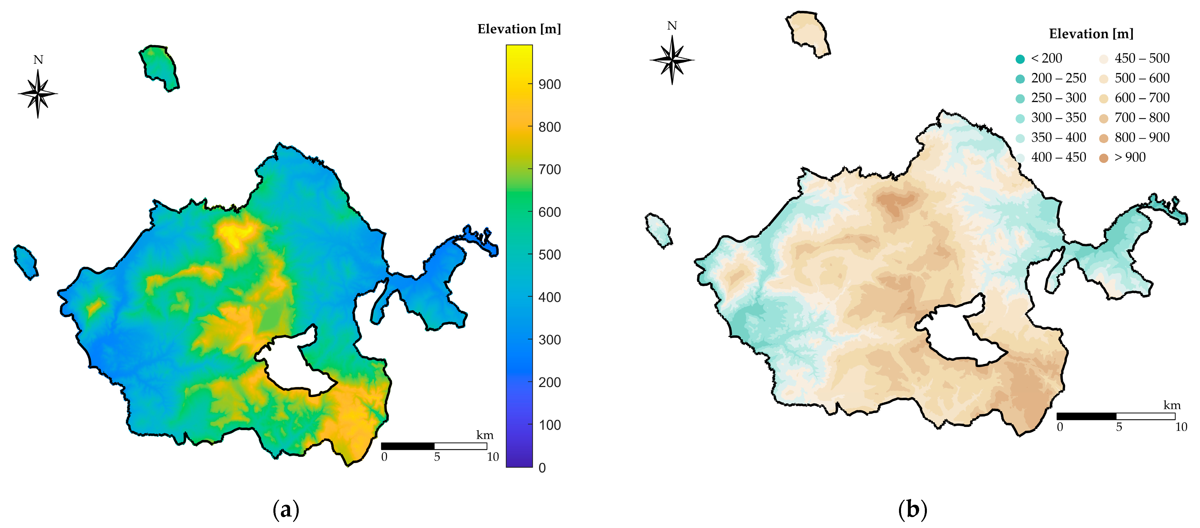
2.1. Digital Terrain Model (Raster File)
info = wmsinfo(UrlMap);
orthoLayer = info.Layer(1);
[E, R] = wmsread(orthoLayer, ‘LatLim’, [LatMin,LatMax], ‘LonLim’,[LongMin,LongMax], ‘CellSize’,CellExtent);
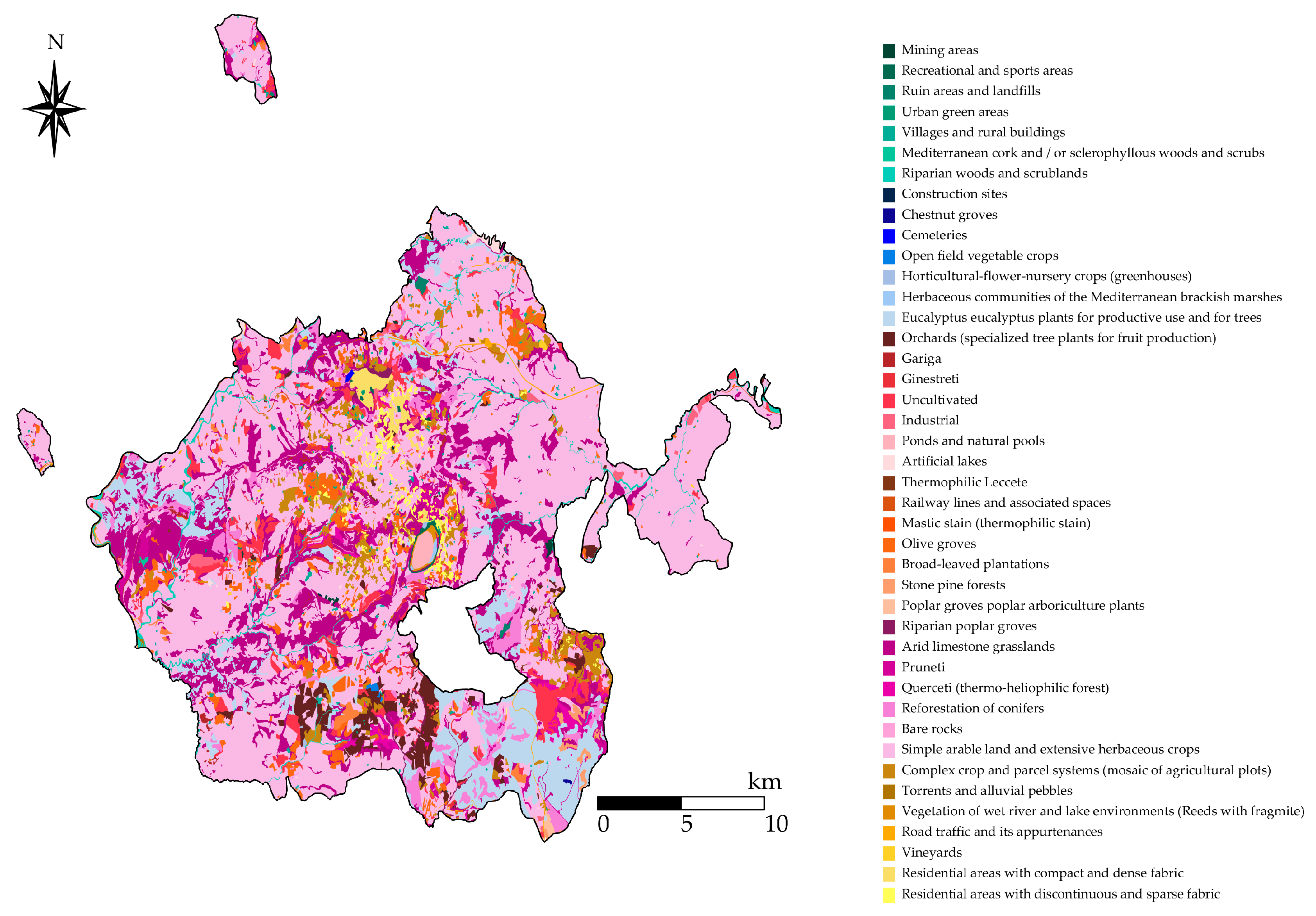
2.2. Lithology and Land Use Import (Shapefile)
cat(2,ReadShape.X), cat(2,ReadShape.Y))
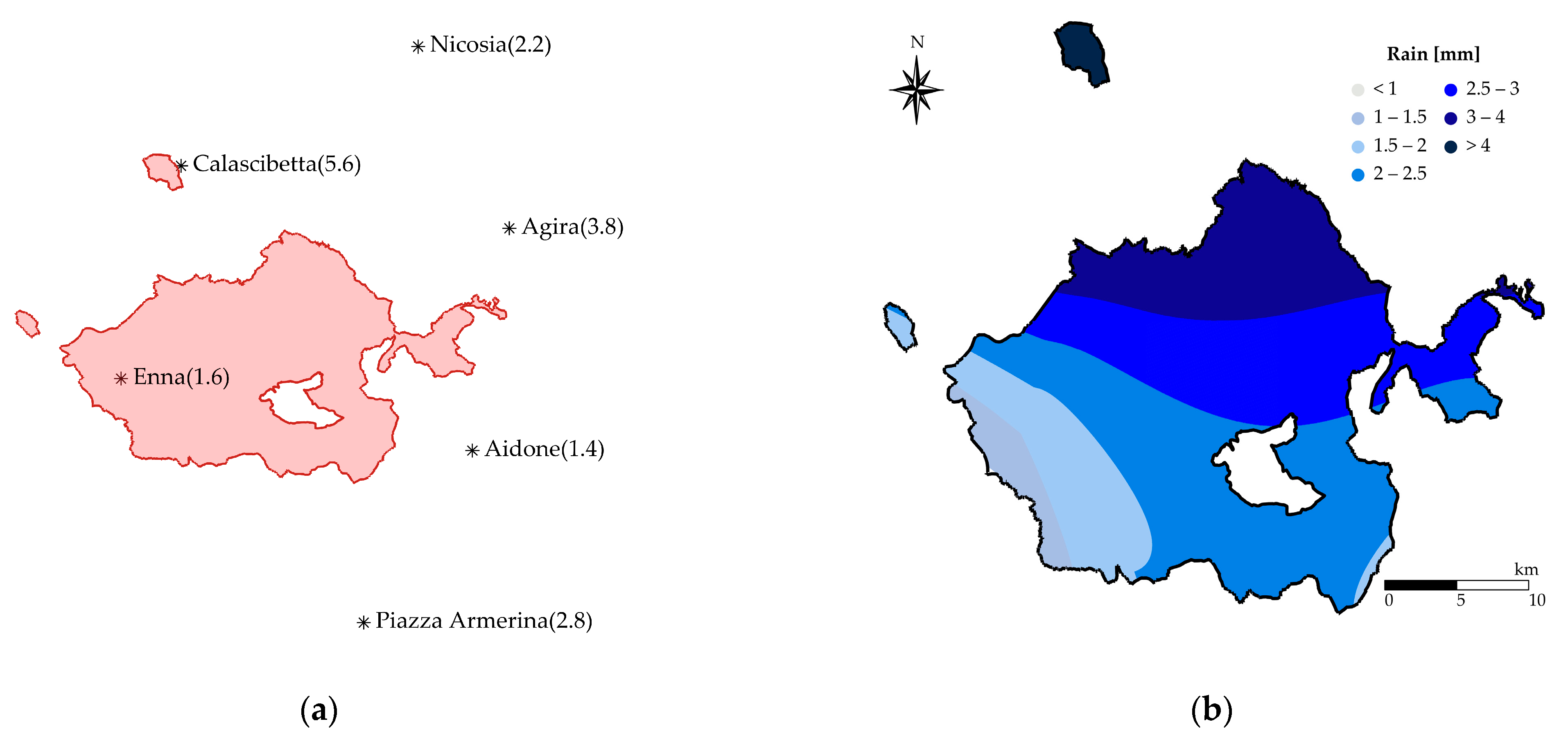
2.3. Rainfall (Point Data)
2.4. Other Useful Operations
2.4.1. Geoprocessing Procedures
2.4.2. Geometric Measurement
2.4.3. User-Defined Parameter Classification
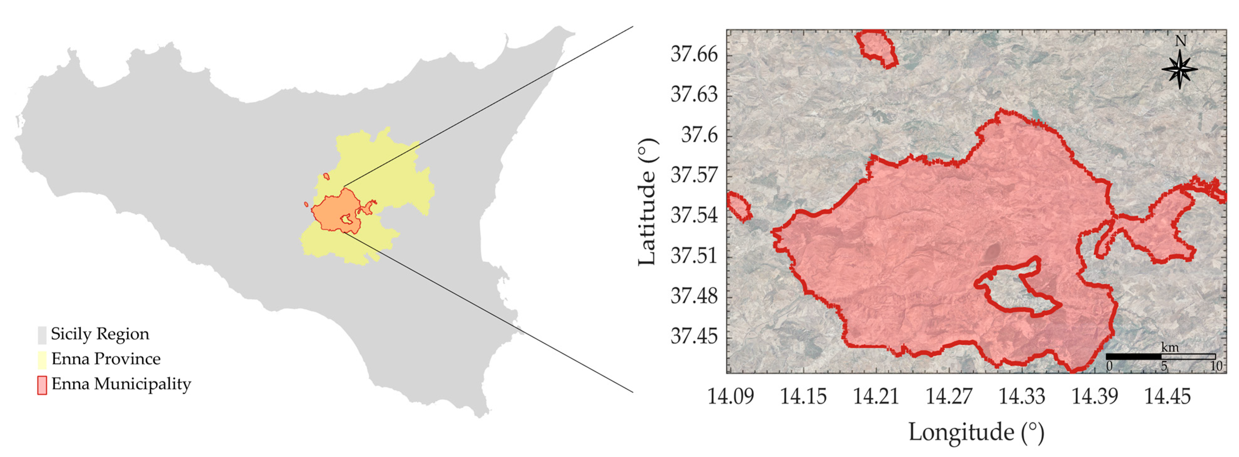
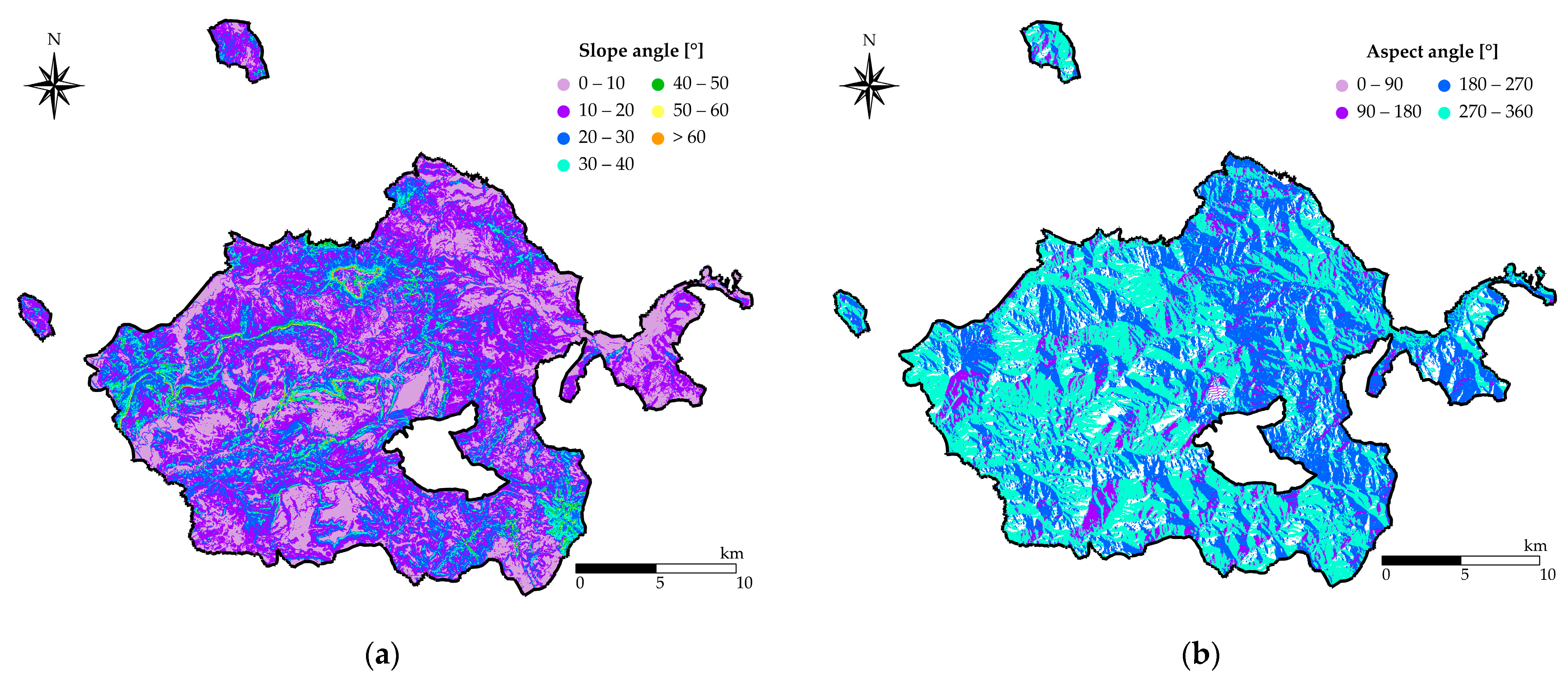
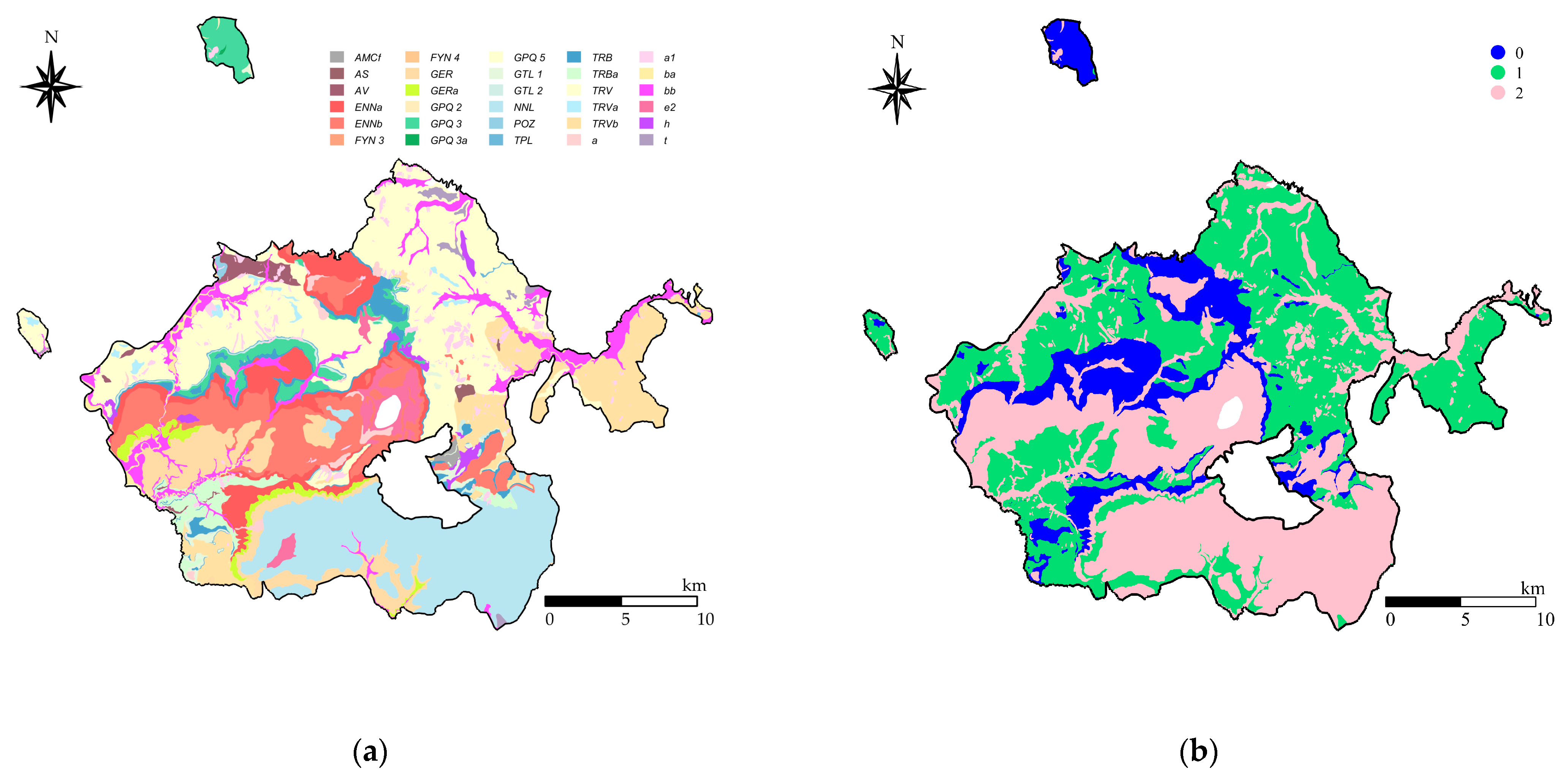
3. The Conditioning Factors for a Landslide Susceptibility Assessment of Enna Municipality (Sicily, Italy)
4. Discussion
Author Contributions
Funding
Institutional Review Board Statement
Informed Consent Statement
Data Availability Statement
Conflicts of Interest
References
- Varnes, D.J. Slope movement types and processes. In Landslides, Analysis and Control, Special Report 176: Transportation Research Board; Schuster, R.L., Krizek, R.J., Eds.; National Academy of Sciences: Washington, DC, USA, 1978. [Google Scholar]
- Haque, U.; Da Silva, P.F.; Devoli, G.; Pilz, J.; Zhao, B.; Khaloua, A.; Wilopo, W.; Andersen, P.; Lu, P.; Lee, J.; et al. The human cost of global warming: Deadly landslides and their triggers (1995–2014). Sci. Total Environ. 2019, 682, 673–684. [Google Scholar] [CrossRef] [PubMed]
- Shano, L.; Raghuvanshi, T.K.; Meten, M. Landslide susceptibility evaluation and hazard zonation techniques—A review. Geoenviron. Disasters 2020, 7, 18. [Google Scholar] [CrossRef]
- Roccati, A.; Paliaga, G.; Luino, F.; Faccini, F.; Turconi, L. GIS-Based Landslide Susceptibility Mapping for Land Use Planning and Risk Assessment. Land 2021, 10, 162. [Google Scholar] [CrossRef]
- Lee, S.; Pradhan, B. Landslide hazard mapping at Selangor, Malaysia using frequency ratio and logistic regression models. Landslides 2007, 4, 33–41. [Google Scholar] [CrossRef]
- Yalcin, A.; Reis, S.; Aydinoglu, A.C.; Yomralioglu, T. A GIS-based comparative study of frequency ratio, analytical hierarchy process, bivariate statistics and logistics regression methods for landslide susceptibility mapping in Trabzon, NE Turkey. Catena 2011, 85, 274–287. [Google Scholar] [CrossRef]
- Felicisimo, Á.M.; Cuartero, A.; Remondo, J.; Quirós, E. Mapping landslide susceptibility with logistic regression, multiple adaptive regression splines, classification and regression trees, and maximum entropy methods: A comparative study. Landslides 2012, 10, 175–189. [Google Scholar] [CrossRef]
- Li, L.; Lan, H.; Guo, C.; Zhang, Y.; Li, Q.; Wu, Y. A modified frequency ratio method for landslide susceptibility assessment. Landslides 2017, 14, 727–741. [Google Scholar] [CrossRef]
- Wang, Q.; Li, W. A GIS-based comparative evaluation of analytical hierarchy process and frequency ratio models for landslide susceptibility mapping. Phys. Geogr. 2017, 38, 318–337. [Google Scholar] [CrossRef]
- Mersha, T.; Meten, M. GIS-based landslide susceptibility mapping and assessment using bivariate statistical methods in Simada area, northwestern Ethiopia. Geoenviron. Disasters 2020, 7, 20. [Google Scholar] [CrossRef]
- Eiras, C.G.S.; Souza, J.R.G.; Freitas, R.D.A.; Barella, C.F.; Pereira, T.M. Discriminant analysis as an efficient method for landslide susceptibility assessment in cities with the scarcity of predisposition data. Nat. Hazards 2021, 107, 1427–1442. [Google Scholar] [CrossRef]
- Montrasio, L. Stability analysis of soil slip. In Proceedings of the International Conference Risk, Munich, Germany, 15–18 October 2000; Brebbia, C.A., Ed.; Wit Press, Southampton: Boston, MA, USA, 2000. [Google Scholar]
- Goetz, J.N.; Guthrie, R.H.; Brenning, A. Integrating physical and empirical landslide susceptibility models using generalized additive models. Geomorphology 2011, 129, 376–386. [Google Scholar] [CrossRef]
- Ghosh, S.; Carranza, E.J.M.; van Westen, C.J.; Jetten, V.G.; Bhattacharya, D.N. Selecting and weighting spatial predictors for empirical modeling of landslide susceptibility in the Darjeeling Himalayas (India). Geomorphology 2011, 131, 35–56. [Google Scholar] [CrossRef]
- Montrasio, L.; Valentino, R.; Losi, G.L. Towards a real-time susceptibility assessment of rainfall-induced shallow landslides on a regional scale. Nat. Hazards Earth Syst. Sci. 2011, 11, 1927–1947. [Google Scholar] [CrossRef] [Green Version]
- Montrasio, L.; Valentino, R.; Corina, A.; Rossi, L.; Rudari, R. A prototype system for space–time assessment of rainfall-induced shallow landslides in Italy. Nat. Hazards 2014, 74, 1263–1290. [Google Scholar] [CrossRef]
- Formetta, G.; Capparelli, G.; Versace, P. Evaluating performance of simplified physically based models for shallow landslide susceptibility. Hydrol. Earth Syst. Sci. 2016, 20, 4585–4603. [Google Scholar] [CrossRef] [Green Version]
- Gutiérrez-Martín, A. A GIS-physically-based emergency methodology for predicting rainfall-induced shallow landslide zonation. Geomorphology 2020, 359, 107121. [Google Scholar] [CrossRef]
- Medina, V.; Hürlimann, M.; Guo, Z.; Lloret, A.; Vaunat, J. Fast physically-based model for rainfall-induced landslide susceptibility assessment at regional scale. Catena 2021, 201, 105213. [Google Scholar] [CrossRef]
- Peng, L.; Niu, R.; Huang, B.; Wu, X.; Zhao, Y.; Ye, R. Landslide susceptibility mapping based on rough set theory and support vector machines: A case of the three gorges area, China. Geomorphology 2014, 204, 287–301. [Google Scholar] [CrossRef]
- Arnone, E.; Francipane, A.; Scarbaci, A.; Puglisi, C.; Noto, L.V. Effect of raster resolution and polygon-conversion algorithm on landslide susceptibility mapping. Environ. Model. Softw. 2016, 84, 467–481. [Google Scholar] [CrossRef]
- Ortiz, J.A.V.; Martínez-Graña, A.M. A neural network model applied to landslide susceptibility analysis (Capitanejo, Colombia). Geomat. Nat. Hazards Risk. 2018, 9, 1106–1128. [Google Scholar] [CrossRef] [Green Version]
- Chen, W.; Shahabi, H.; Shirzadi, A.; Hong, H.; Akgun, A.; Tian, Y.; Liu, J.; Zhu, A.; Li, S. Novel hybrid artificial intelligence approach of bivariate statistical-methods-based kernel logistic regression classifier for landslide susceptibility modeling. Bull. Eng. Geol. Environ. 2019, 78, 4397–4419. [Google Scholar] [CrossRef]
- Bragagnolo, L.; da Silva, R.V.; Grzybowski, J.M.V. Artificial neural network ensembles applied to the mapping of landslide susceptibility. Catena 2020, 184, 104240. [Google Scholar] [CrossRef]
- Sufi, F.K. AI-Landslide: Software for acquiring hidden insights from global landslide data using Artificial Intelligence. Softw. Impacts 2021, 10, 100177. [Google Scholar] [CrossRef]
- Kamran, K.V.; Feizizadeh, B.; Khorrami, B.; Ebadi, Y. A comparative approach of support vector machine kernel functions for GIS-based landslide susceptibility mapping. Appl. Geomat. 2021, 13, 837–851. [Google Scholar] [CrossRef]
- Ali, S.A.; Parvin, F.; Vojteková, J.; Costache, R.; Linh, N.T.T.; Pham, Q.B.; Vojtek, M.; Gigović, L.; Ahmad, A.; Ghorbani, M.A. GIS-based landslide susceptibility modeling: A comparison between fuzzy multi-criteria and machine learning algorithms. Geosci. Front. 2021, 12, 857–876. [Google Scholar] [CrossRef]
- Ma, Z.; Mei, G.; Piccialli, F. Machine learning for landslides prevention: A survey. Neural. Comput. Appl. 2021, 33, 10881–10907. [Google Scholar] [CrossRef]
- Pham, Q.B.; Achour, Y.; Ali, S.A.; Parvin, F.; Vojtek, M.; Vojteková, J.; Al-Ansari, N.; Achu, A.L.; Costache, R.; Khedher, K.M.; et al. A comparison among fuzzy multi-criteria decision making, bivariate, multivariate and machine learning models in landslide susceptibility mapping. Geomat. Nat. Hazards Risk. 2021, 12, 1741–1777. [Google Scholar] [CrossRef]
- Youssef, A.M.; Pourghasemi, H.R. Landslide susceptibility mapping using machine learning algorithms and comparison of their performance at Abha Basin, Asir Region, Saudi Arabia. Geosci. Front. 2021, 12, 639–655. [Google Scholar] [CrossRef]
- Rahaman, A.; Venkatesan, M.S.; Ayyamperumal, R. GIS-based landslide susceptibility mapping method and Shannon entropy model: A case study on Sakaleshapur Taluk, Western Ghats, Karnataka, India. Arab. J. Geosci. 2021, 14, 2154. [Google Scholar] [CrossRef]
- Zhao, P.; Masoumi, Z.; Kalantari, M.; Aflaki, M.; Mansourian, A. A GIS-Based Landslide Susceptibility Mapping and Variable Importance Analysis Using Artificial Intelligent Training-Based Methods. Remote Sens. 2022, 14, 211. [Google Scholar] [CrossRef]
- Carrara, A. A multivariate model for landslide hazard evaluation. Math. Geol. 1983, 15, 403–426. [Google Scholar] [CrossRef]
- Meijerink, A.M.J. Data acquisition and data capture through terrain mapping unit. Int. Comput. J. 1988, 1, 23–44. [Google Scholar]
- Pike, R.J. The geometric signature: Quantifying landslide terrain types from digital elevation models. Math. Geol. 1988, 20, 491–511. [Google Scholar] [CrossRef]
- Carrara, A.; Cardinali, M.; Detti, R.; Guzzetti, F.; Pasqui, V.; Reichenbach, P. GIS techniques and statistical models in evaluating landslide hazard. Earth Surf. Process. Landf. 1991, 16, 427–445. [Google Scholar] [CrossRef]
- Van Westen, C.J. Application of Geographical Information System to Landslide Hazard Zonation. Ph.D. Thesis, ITC Publication, Enschede, The Netherlands, 1993. [Google Scholar]
- Hearn, G.J.; Griffiths, J.S. Landslide hazard mapping and risk assessment. Geol. Soc. Spec. Publ. 2001, 18, 43–52. [Google Scholar] [CrossRef]
- Lee, S.; Min, K. Statistical analysis of landslide susceptibility at Yongin, Korea. Environ. Geol. 2001, 40, 1095–1113. [Google Scholar] [CrossRef]
- Ba, Q.; Chen, Y.; Deng, S.; Yang, J.; Li, H. A comparison of slope units and grid cells as mapping units for landslide susceptibility assessment. Earth Sci. Inform. 2018, 11, 373–388. [Google Scholar] [CrossRef]
- Hormann, K.; Agathos, A. The point in polygon problem for arbitrary polygons. Comput. Geom. 2001, 20, 131–144. [Google Scholar] [CrossRef] [Green Version]
- Kepner, J.; Kipf, A.; Engwirda, D.; Vembar, N.; Jones, M.; Milechin, L.; Gadepally, V.; Hill, C.; Kraska, T.; Arcand, W.; et al. Fast Mapping onto Census Blocks. In Proceedings of the 2020 IEEE High Performance Extreme Computing Conference, Waltham, MA, USA, 22–24 September 2020. [Google Scholar] [CrossRef]
- Engwirda, D. Locally-Optimal Delaunay-Refinement and Optimisation-Based Mesh Generation. Ph.D. Thesis, The University of Sydney, Sydney, Australia, 2014. Available online: http://hdl.handle.net/2123/13148 (accessed on 5 November 2021).
- Schlining, B.; Signell, R.; Crosby, A. Nctoolbox (2009), Github Repository. Available online: https://github.com/nctoolbox/nctoolbox (accessed on 10 September 2021).
- Cheng, M.; Wang, Y.; Engel, B.; Zhang, W.; Peng, H.; Chen, X.; Xia, H. Performance Assessment of Spatial Interpolation of Precipitation for Hydrological Process Simulation in the Three Gorges Basin. Water 2017, 9, 838. [Google Scholar] [CrossRef] [Green Version]
- Yoshpe, M. Distance from Points to Polyline or Polygon, MATLAB Central File Exchange. 28 January 2022. Available online: https://www.mathworks.com/matlabcentral/fileexchange/12744-distance-from-points-to-polyline-or-polygon (accessed on 10 January 2022).
- Castelli, F.; Castellano, E.; Contino, F.; Lentini, V. A Web-based GIS system for landslide risk zonation: The case of Enna area (Italy). In Proceedings of the 12th International Symposium on Landslides, Napoli, Italy, 12–19 June 2016. [Google Scholar]
- Castelli, F.; Freni, G.; Lentini, V.; Fichera, A. Modelling of a debris flow event in the Enna area for hazard assessment. In Proceedings of the 1st International Conference on the Material Point Method (MPM 2017), Delft, The Netherlands, 10–13 January 2017; Volume 175, pp. 287–292. [Google Scholar]
- Lentini, V.; Distefano, G.; Castelli, F. Consequence analyses induced by landslides along transport infrastructures in the Enna area (South Italy). Bull. Eng. Geol. Environ. 2019, 78, 4123–4138. [Google Scholar] [CrossRef]
- Ottens, H.F.L. GIS in Europe. In Proceedings of the II European Conference on GIS, Brussels, Belgium, 2–5 April 1991; Volume 1, pp. 1–9. [Google Scholar]


| Format | Function |
|---|---|
| .tif + .tfw | E = imread(‘.tif’) R = worldfileread(‘.tfw’, ‘planar’, size(E)) |
| .tif (GeoTiff) .asc | [E, R] = readgeoraster(‘.tif/.asc’, ‘OutputType’, ‘double’) |
| Lithological Code | Denomination | Description | Class |
|---|---|---|---|
| AMCf | Centuripe formation | Blue marly clay | 1 |
| AS | Scaly clay | Scaly clay | 1 |
| AV | Variegated clay | Variegated clay | 1 |
| ENNa | Enna formation | Marl and clayey marl | 0 |
| ENNb | Enna formation | Sand and Limestone | 2 |
| FYN3 | Numidian flysh | Blackish clay, brown clay and yellowish quartz sandstone | 1 |
| FYN4 | Numidian flysch | Quartz, kaolinitic mudstones and silty clay | 1 |
| GER | Geracello formation | Marly clay | 1 |
| GERa | Geracello formation | Sandy clay and clayey sand | 2 |
| GPQ2 | Pasquasia formation | Gypsum arenite | 2 |
| GPQ3 | Pasquasia formation | Marly gypsum | 0 |
| GPQ 3a | Pasquasia formation | Gypsum | 0 |
| GPQ5 | Pasquasia formation | Sandy-gypsum brownish clays | 1 |
| GTL1 | Cattolica formation | Limestone | 0 |
| GTL2 | Cattolica formation | Selenite | 0 |
| NNL | Lannari formation | Medium/fine-grained sand | 2 |
| POZ | Polizzi formation | Calciluties | 0 |
| TPL | Tripoli | Laminated diatomites | 0 |
| TRB | Trubi | Calcareous marl and marly limestone | 0 |
| TRBa | Trubi | Claystone breccias and brecciated clays | 1 |
| TRV | Terravecchia formation | Clayey marl and marly-silty clay | 1 |
| TRVa | Terravecchia formation | Conglomerates | 0 |
| TRVb | Terravecchia formation | Claystone breccias and brecciated clays | 1 |
| a | Colluvium deposits | Sand with many cobbles and boulders | 2 |
| a1 | Landslide deposits | Heterogeneous materials | 2 |
| ba | Alluvial deposits | Gravel, sand and clayey silt | 2 |
| bb | Recent alluvial deposits | Medium-fine grained sand | 2 |
| e2 | Lacustrine deposits | Sandy loam | 2 |
| h | Anthropic deposits | Gravel, sand, silt, clay | 2 |
| t | Alluvial terrace deposits | Gravel, sand, silt, clay | 2 |
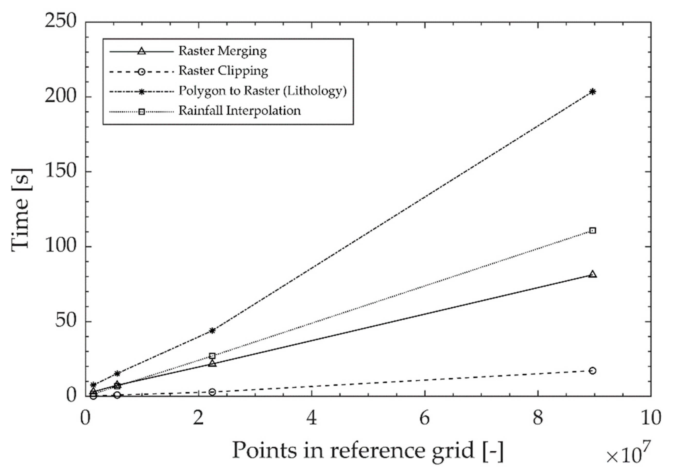
| Raster Samples (-) | Merging, Data Store in Cell Array and Computing of Geomorphology Parameters (s) | Clipping (s) | Polygon to Raster Conversion (inpoly) (s) | Rainfall Interpolation (s) |
|---|---|---|---|---|
| 83,656,084 (2 × 2 m) | 81.21 | 17.17 | 203.60 | 110.74 |
| 22,420,209 (4 × 4 m) | 21.70 | 2.95 | 43.92 | 27.01 |
| 5,609,137 (8 × 8 m) | 7.49 | 0.92 | 15.30 | 6.75 |
| 1,403,860 (16 × 16 m) | 3.13 | 0.28 | 7.59 | 1.75 |
Publisher’s Note: MDPI stays neutral with regard to jurisdictional claims in published maps and institutional affiliations. |
© 2022 by the authors. Licensee MDPI, Basel, Switzerland. This article is an open access article distributed under the terms and conditions of the Creative Commons Attribution (CC BY) license (https://creativecommons.org/licenses/by/4.0/).
Share and Cite
Gatto, M.P.A.; Misiano, S.; Montrasio, L. On the Use of MATLAB to Import and Manipulate Geographic Data: A Tool for Landslide Susceptibility Assessment. Geographies 2022, 2, 341-353. https://doi.org/10.3390/geographies2020022
Gatto MPA, Misiano S, Montrasio L. On the Use of MATLAB to Import and Manipulate Geographic Data: A Tool for Landslide Susceptibility Assessment. Geographies. 2022; 2(2):341-353. https://doi.org/10.3390/geographies2020022
Chicago/Turabian StyleGatto, Michele Placido Antonio, Salvatore Misiano, and Lorella Montrasio. 2022. "On the Use of MATLAB to Import and Manipulate Geographic Data: A Tool for Landslide Susceptibility Assessment" Geographies 2, no. 2: 341-353. https://doi.org/10.3390/geographies2020022
APA StyleGatto, M. P. A., Misiano, S., & Montrasio, L. (2022). On the Use of MATLAB to Import and Manipulate Geographic Data: A Tool for Landslide Susceptibility Assessment. Geographies, 2(2), 341-353. https://doi.org/10.3390/geographies2020022