Map Projections Classification

Abstract

Many books, textbooks and papers have been published in which the classification of map projections is based on auxiliary (developable) surfaces and projections are divided into conic, cylindrical and azimuthal projections. We argue that such a classification of map projections is unacceptable and give many reasons for that. Many authors wrote in more detail about the classification of map projections, and our intention is to give a new refined and rectified insight into the classification of map projections. Our approach can be included in map projection publications of general and thematic cartography. Doing this, misconceptions and unnecessary insistence on conceptuality instead of reality will be avoided.

1. Introduction

So far, many books and textbooks of general, thematic and even mathematical cartography have been published, as well as articles in journals, in which one of the classifications of map projections is based on auxiliary (developable) surfaces and projections are divided into conic, cylindrical and azimuthal projections. This classification is illustrated by images in which the surface of a cone and the surface of a cylinder or a plane touch or intersect the Earth’s sphere (Figure 1).

When searching for a term, many of us will first look for a solution on the Internet, and most often it will be Wikipedia. We can find this description there: “A fundamental projection classification is based on the type of projection surface onto which the globe is conceptually projected. The projections are described in terms of placing a gigantic surface in contact with the Earth, followed by an implied scaling operation. These surfaces are cylindrical (e.g., Mercator), conic (e.g., Albers), and plane (e.g., stereographic). Many mathematical projections, however, do not neatly fit into any of these three conceptual projection methods.” [1]. The same or very similar approach can be found in many references, e.g., in [2,3,4,5,6,7,8,9,10,11,12].

There are several reasons why this classification of map projections is not recommended.

1.1. History

• The authors of the oldest known cylindrical and conic projections did not define their projections using indirect, developable surfaces. For example, Mercator, in the 16th century, did not use a cylindrical surface to define the projection now called Mercator’s cylindrical projection, or Lambert, in the 18th century, did not use a conical surface to define the projection now called Lambert’s conformal conic projection. On the contrary, after deriving the equations of that projection, Lambert [13] mentioned that the map made in that projection could be folded into a cone.
• It seems that developable surfaces related to map projections appear for the first time in the second half of the 19th century. D’Avezac-Macaya [4] referred to “les projections perspectives, les developements de surfaces osculatrices ou pénétrantes”, that is, tangent or secant surfaces, specifically “les développements cylindriques” and “cóniques”, and the catch-all “les systèmes conventionneles”. Snyder [3] did not find any earlier cartographic references to developable surfaces. Let us mention the famous older authors who dealt with map projections, not to mention developable surfaces: Lambert [13], Euler [14], Lagrange [15], Gauss [16] and Tissot [17].

1.2. Conceptuality

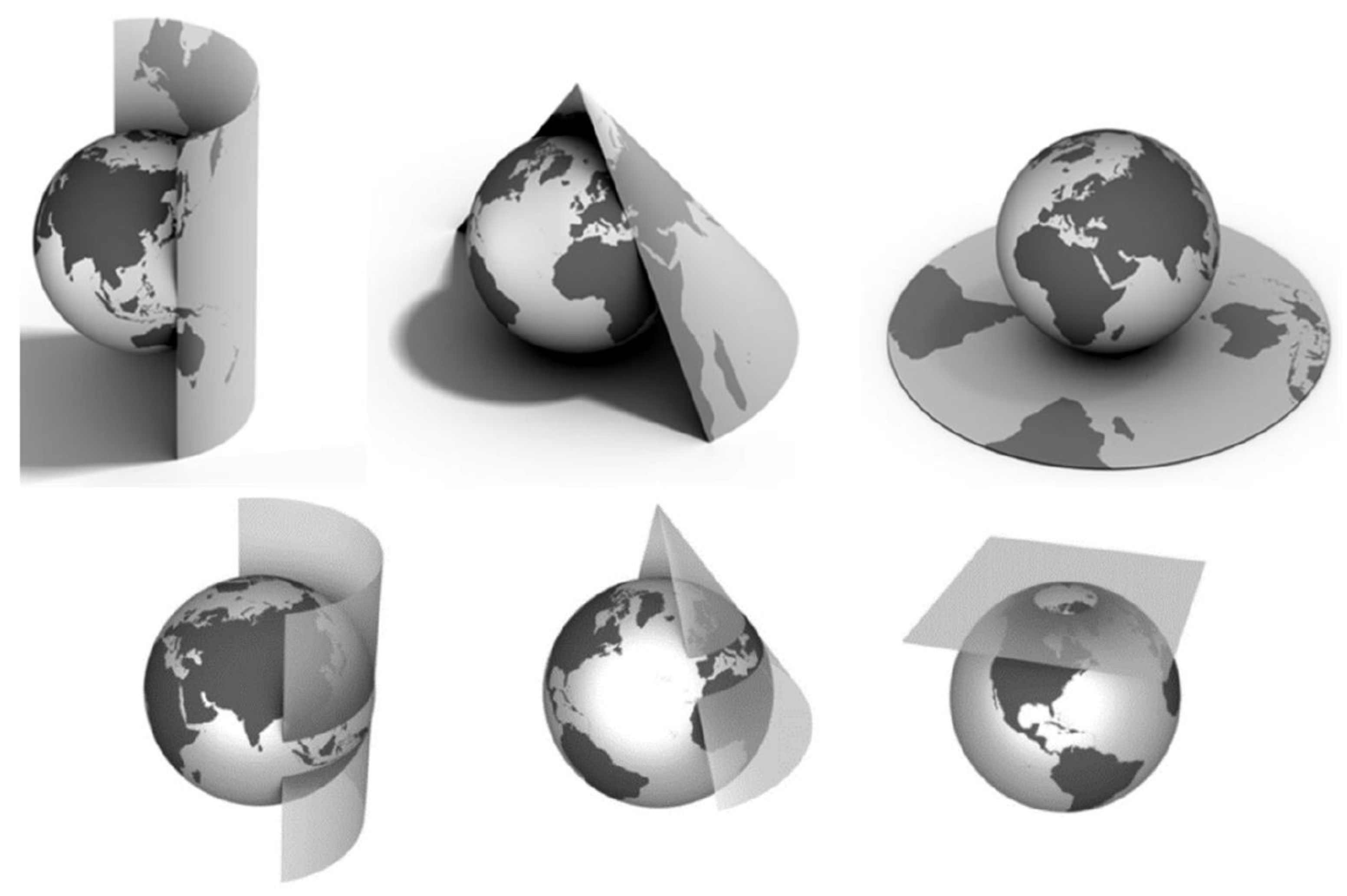
• One of the most common classifications, and the one principally used by Snyder [3], is based on association, at least conceptually, to a developable surface.
• Map projections are mappings of a curved surface, most often a sphere or ellipsoid, into a plane. The introduction of developable surfaces as intermediate surfaces and the interpretation according to which a sphere or ellipsoid is first mapped to such a surface which then develops into a plane is a fabrication that generally does not correspond to reality. It is usually justified by the term conceptual [2] and explained by the claim that map projections are easier to interpret in this way.
• “The reference globe and developable surfaces are conceptual aids that help illustrate the projection process, but they are not used to create projections today. Rather, the field of mathematics is utilized to create projections, and so it is important to understand some of the basic mathematical manipulations used to project the Earth onto a map.” [9]. The first part of the first sentence is questionable because developable surfaces are not used in the projection process, in general. The rest of the quotation we fully accept. As everybody can see, there are no developable surfaces in the whole chapter 8.3 of the cited book.
• “The classification of projections according to developable surfaces (cylinder, cone, and plane) is useful for the comprehension of selecting projections and their parameters. However, while developable surfaces are a useful conceptual tool, it needs to be emphasized that most map projections cannot be constructed geometrically but are instead defined mathematically” [18]. It remains unclear why Šavrič et al. [18] mentioned the classification of map projections using developable surfaces when they are not used in their Projection Wizard.
• “While the concept of developable surfaces provides a nice way to visualize the basics of map projections, as stated before, the transformation is really driven by mathematical equations” [10]. The basics of map projections are not connected to developable surfaces at all.

1.3. Prior Warning

• This approach to the classification of map projections is common. Map projections are typically classified according to the geometric surface from which they are derived: cylinder, cone or plane. However, such an approach is only correct at first glance. In fact, the opposite is true. Cylindrical projections are not called so because of the mapping on a cylindrical surface but because the map made in such a projection can be bent into a cylinder. Similarly, conic projections are not called so because of mapping to a conical surface but because a map made in a conic projection can be bent into a cone. More than 100 years ago, in a paper on map projections, Close and Clarke [19] wrote: “Conical projections are those in which the parallels are represented by concentric circles and the meridians by equally spaced radii. There is no necessary connexion between a conical projection and any touching or secant cone. The name conical is given to the group embraced by the above definition, because as is obvious, a projection so drawn can be round to form a cone.” In a well-known paper on the nomenclature and classification of map projections, Lee [20] explained: “Cylindric: projections in which the meridians are represented as a system of equidistant parallel straight lines, and the parallels by a system of parallel straight lines at right angles to the meridians.
  • Conic: projections in which the meridians are represented as...
  • Azimuthal: projections in which the meridians are represented as...

No reference has been made in the above definitions to cylinders, cones or planes. The projections are termed cylindric or conic because they can be regarded as developed on a cylinder or cone, as the case may be, but it is as well to dispense with picturing cylinders and cones, since they have given rise to much misunderstanding.”

1.4. Isometry

• Authors who nowadays describe map projections in great detail with the help of developable surfaces may not even be aware of the fact that, in this way, they introduce double mappings into the theory of map projections. First, the Earth’s sphere is mapped to the auxiliary developable surface, and then it is transformed in some way, e.g., by development, into a map in the plane. Double mappings have their role in the theory of map projections in some special cases, not in general. One should know that developing into a plane is isometry, i.e., such a mapping that preserves distances.
• The use of development surfaces in the definition of map projection is justified only for a small number of projections, projections in which the mapping is real and not conceptual to the corresponding developable surface. Namely, in addition to cylindrical and conic projections, there are many others, such as azimuthal, pseudocylindrical, pseudoconic, conditional, etc., which cannot be interpreted by mapping to a cylinder or cone surface. There are some attempts in that direction. For example, it is said that a pseudocylindrical projection is a mapping to a pseudocylinder but without saying what a pseudocylinder is [7]. Or that such a projection is interpreted as a mapping to an oval surface, without noticing that it is not a developable surface [8].
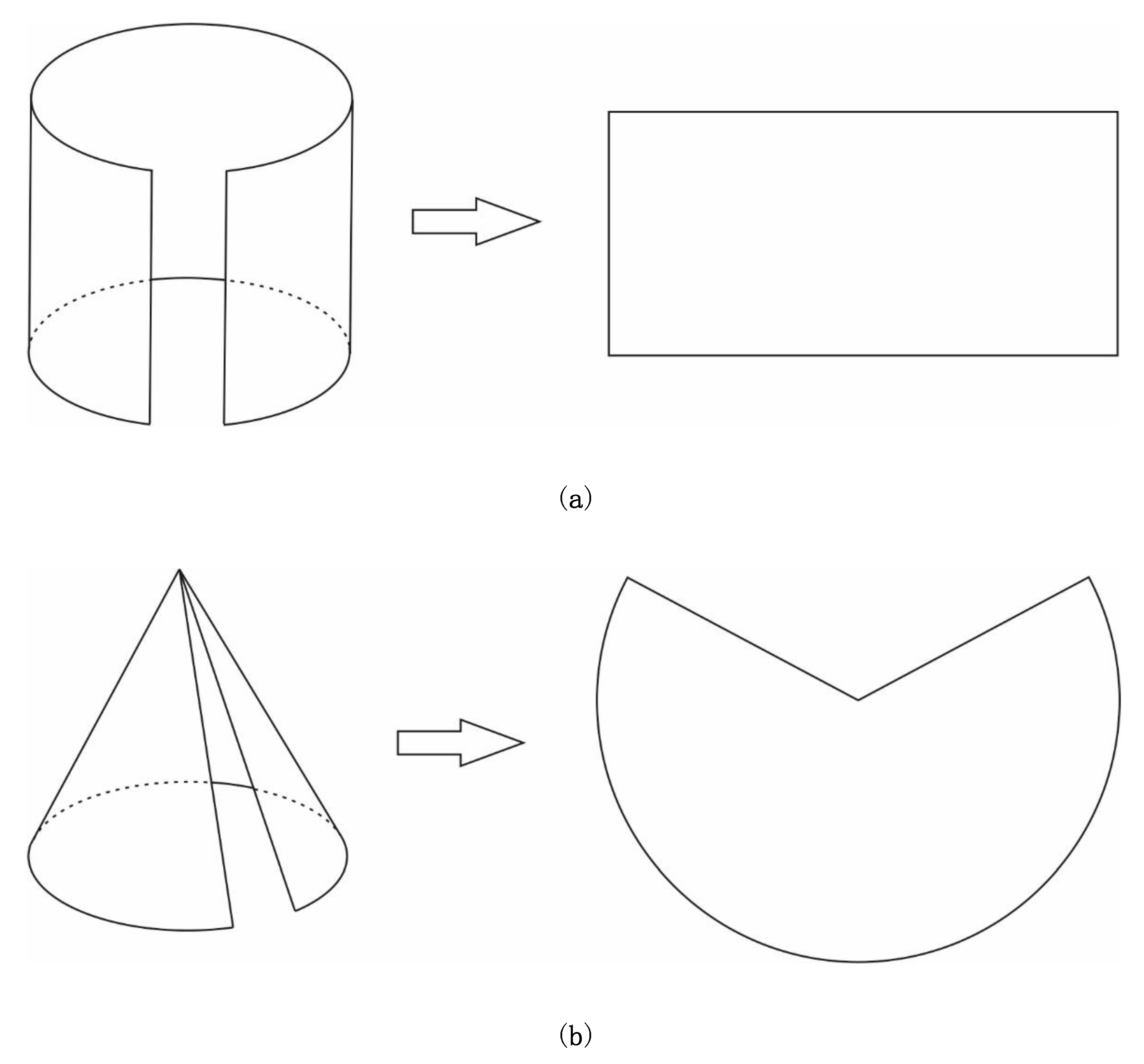
• In the context of the classification of projections into conical, cylindrical and azimuthal/plane, it is unnatural to use a plane as a developable surface. Namely, developing is isometry, and thus we see no purpose in developing plane into plane.
• Developing the auxiliary surface into a plane (Figure 2) preserves distances (isometry). This would then mean that the two selected parallels as standard parallels in all normal aspect projections are mapped to parallels that are at the same distance from each other. Is that possible? Of course not.

1.5. Standard vs. Secant Parallels

• Authors who perceive map projections as mappings with the help of an auxiliary surface regularly distinguish the case of touching and cutting. For them, as a rule, the cross-sectional curve is also a curve without deformations. They take that fact for granted, without proof. However, it has been shown that standard parallels and secant parallels are two different concepts and that they generally do not coincide [21,22,23].
• “Where the ellipsoid and the map projection surface touch, in this case, intersect, there is no distortion. However, between the standard lines the map is under the ellipsoid and outside of them the map is above it.” [5,6]. From this quote, it is clear that van Sickle did not distinguish between secant and standard parallels.
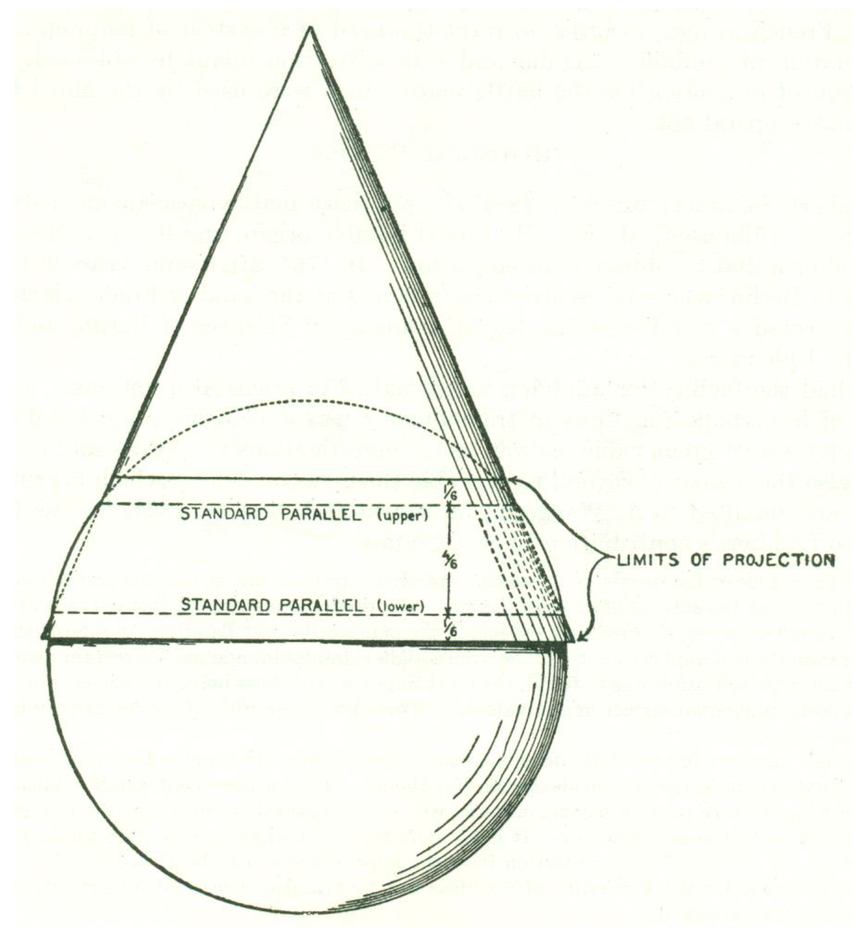
• The use of developable surfaces leads to secant projections, i.e., mappings on the auxiliary developable surface that intersects the mapped surface and thence the conclusion that azimuthal projections can have at most one standard parallel and conic at most two. This is wrong because there are azimuthal and conic projections with several standard parallels [24,25].
• It is generally accepted that a secant projection is a mapping on an auxiliary surface that intersects a sphere or an ellipsoid and that the intersections of the secant conic and cylindrical projection are without deformations (Figure 3). Thus, for example, in ESRI’s dictionary [11], we were able to read several years ago: “Secant projection: A projection whose surface intersects the surface of a globe. A secant conic or cylindrical projection, for example, is recessed into a globe, intersecting it at two circles. At the lines of intersection, the projection is free from distortion.” This definition is not good. First, the intersection of two second-order surfaces is a fourth-order curve that generally does not consist of two circles. However, this shortcoming could be corrected by specifying the mutual position of the surface of the cone or cylinder and the sphere. However, the claim that the line of intersection of two surfaces is free of deformation cannot be an integral part of the definition because, in addition to being a claim, it is generally erroneous. However, it is so ingrained that it is almost regularly taken as true without evidence. The cited webpage is no longer available, but ESRI retains the term secant projection within the definitions of cylindrical and conical projections [11].

1.6. Conclusions

• Instead of a conceptual approach that is also wrong in some parts, it is necessary to return to reality and not run away from mathematics. Let us just recall that the study of map projections was not so long ago called mathematical cartography.
• Explaining the mapping of a sphere or ellipsoid to the surface of a cylinder or cone is a convenient story, which, unfortunately, while avoiding the mathematical background of the process, leads to erroneous claims which, most likely, the authors are not aware of.
• It is possible to communicate perfectly without the introduction of auxiliary surfaces. A good example of this are the books by Bugayevskiy and Snyder [27], Bugayevskiy [28] and Kessler and Battersby [29].

D’Avezac de Castera-Macaya [4], Deetz and Adams [26], Maurer [30], Urmayev [31], Lee [20], Kavrayskiy [32], Tobler [33], Solov’ev [34], Richardus and Adler [35], Maling [36], Konusova [37], Starostin et al. [38], Vakhrameeva et al. [39], Snyder [40], Bugayevskiy and Snyder [27] and Kessler and Battersby [29], for example, wrote in more detail about the classification of map projections. Therefore, it is not our intention to give some new insights into the classification of projections but to write a text that can be included in the chapters on map projections in textbooks of general and thematic cartography and that everything is correct.

2. Map Projections Classification

There is an infinite number of different map projections, and several hundred are known [3]. To make them easier to study and therefore select for practical application, we divide them into groups.

As a basis for the division of map projections are usually taken:

• Properties of mapping or types of distortions;
• The shape of a (pseudo)graticule;
• Projection aspect, i.e., position of the axis of projection in relation to the axis of rotation of the sphere.

2.1. Classification of Map Projections According to Types of Distortions

According to the types of distortions, map projections are divided into these four groups: conformal (equiangular), equivalent (equal-area), equidistant in a certain direction (equal-length) and compromise. Let us define the local linear scale factor as usual:

$$c=\frac{ds\prime }{ds}$$

(1)

where ds′ is a differential of arc length in the plane of projection, and ds is the appropriate differential of arc length on the original surface, usually a sphere or ellipsoid. Analogously, the local area scale factor is

$$p=\frac{dp\prime }{dp}$$

(2)

where dp′ is a differential of an area in the plane of projection, and dp is the appropriate differential of the area on the original surface.

In conformal projections, the distortion of the angles is equal to zero, and the linear scale at a point is equal in all directions, i.e., it does not depend on the azimuth. Because angle distortion in the conformal projections is zero and the scale does not depend on the azimuth at each point, the similarity of the corresponding infinitesimal figures on the ellipsoid and in the plane is maintained, hence their name conformal, i.e., similar in form.

In equal-area projections, the equality of the area of the corresponding figures on the ellipsoid and in the projection is preserved. Therefore, in equal-area projections, the local area scale factor is equal to one in the entire map field.

In equidistant projections, the local linear scale factor is equal to one along one of the main directions, i.e., the directions along which the linear scale has the largest and smallest value. Equidistant projections are in the middle between conformal and equal-area projections by types and magnitudes of distortions. Namely, in equidistant projections, area distortions are smaller than in conformal projections, and angle distortions are smaller than in equal-area projections.

The group of compromise projections includes all those projections that are neither conformal nor equivalent nor equidistant.

2.2. Classification of Projections According to the Shape of the Pseudograticule

The network of pseudomeridians and pseudoparallels (pseudograticule) is obtained by rotating the network of meridians and parallels (graticule) to any other position (Figure 4 and Figure 5). It is obvious that if there is no mentioned rotation, then the pseudograticule coincides with the graticule.

The pseudograticule has the important property that, regardless of the position of the axis, i.e., the aspect of the projection mapped into the plane, it retains the characteristic shape for a particular group of projections and thus allows a unique definition of each group of projections. The following are definitions of the most important groups of projections using a pseudograticule [41,42].

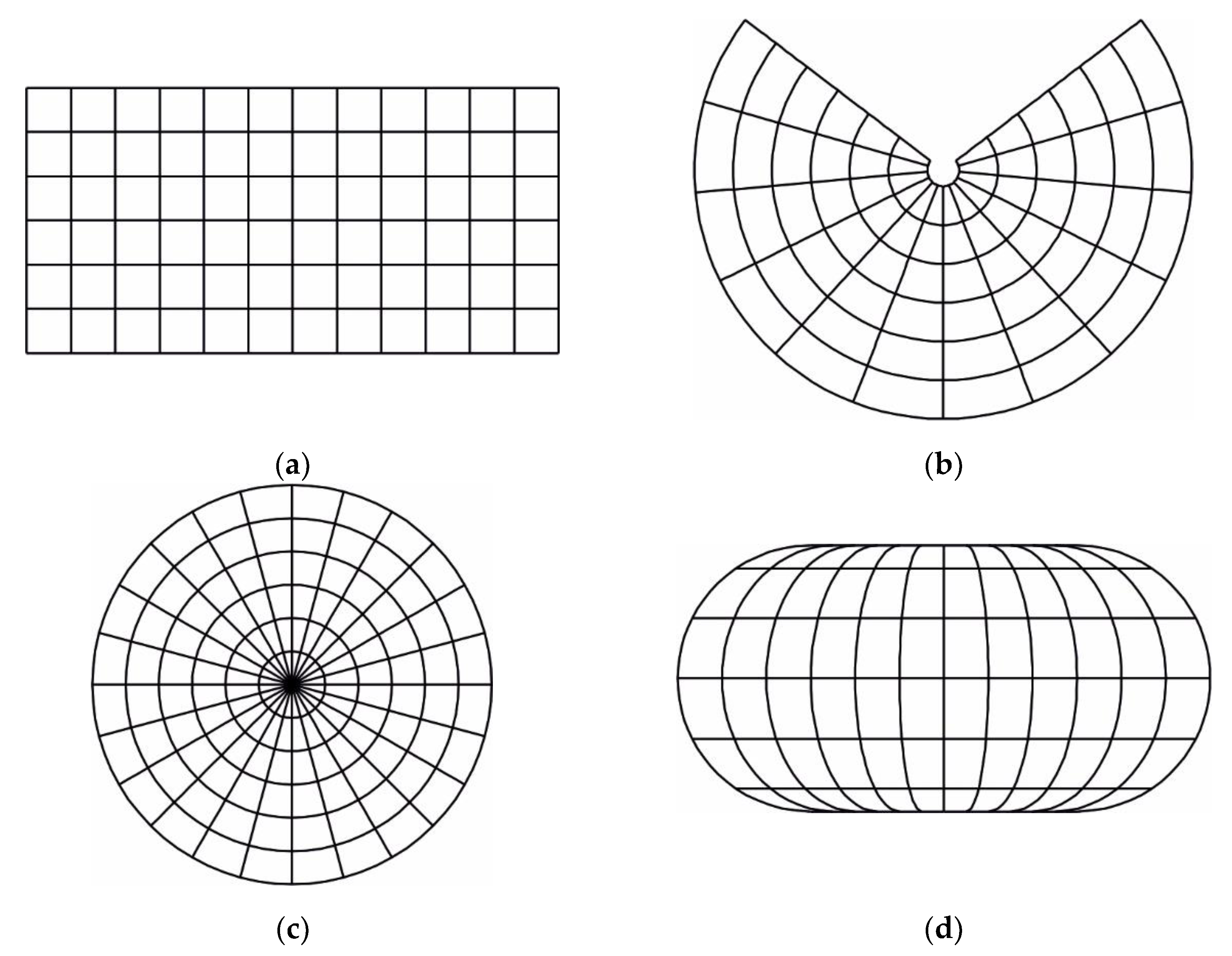
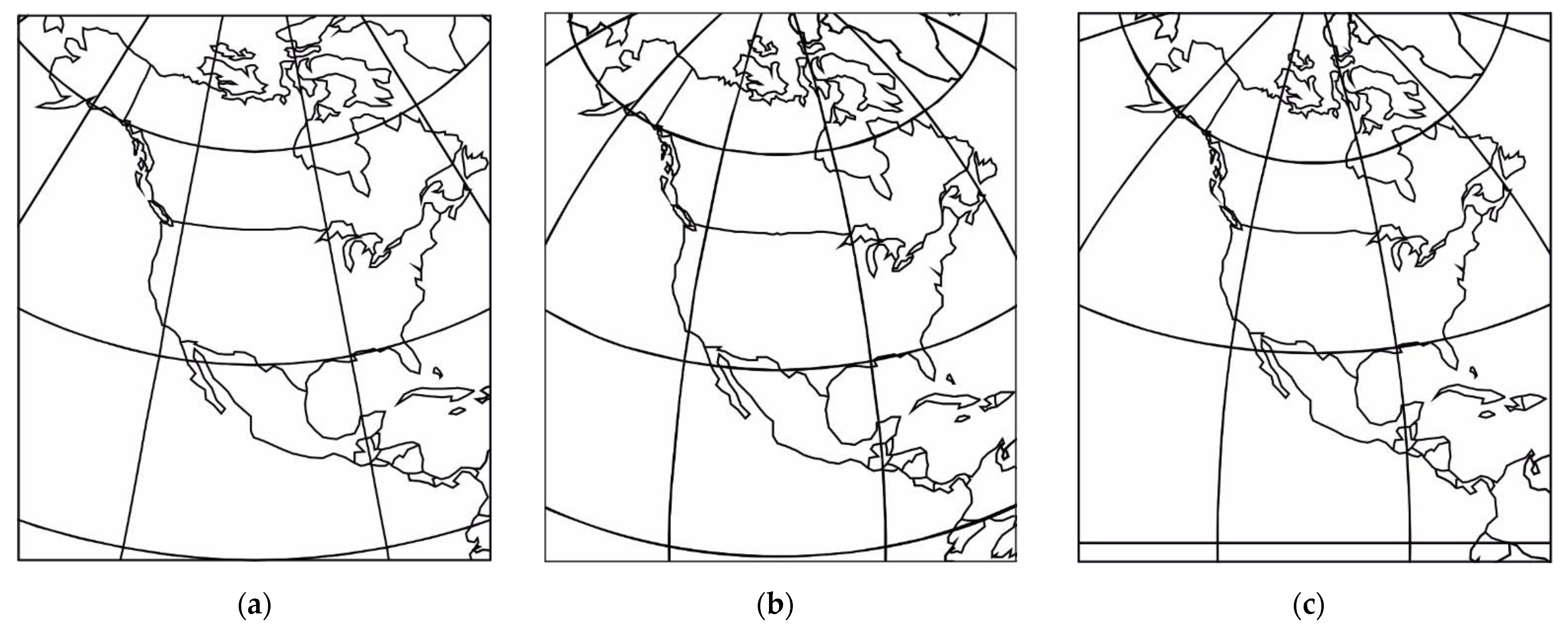
• Cylindrical projections are projections in which pseudomeridians are shown in mutually parallel straight lines and pseudoparallels in mutually parallel straight lines perpendicular to images of pseudomeridians (Figure 6a). Cylindrical projections are not mappings onto a cylindrical surface in general. A map made in a cylindrical projection can be folded into a cylindrical surface.
• Conic projections in the narrower sense are projections in which pseudomeridians are represented by straight lines that intersect at one point and pseudoparallels by concentric circular arcs, with the angle between any two pseudomeridians being less than the difference of the corresponding pseudogeographic longitudes (Figure 6b). Conic projections are not mappings onto a conical surface in general. A map made in a conic projection can be folded into a conical surface.
• Azimuthal projections are projections in which pseudomeridians are shown as straight lines that intersect at one point and pseudoparallels by concentric circles, with the angle between any two pseudomeridians being equal to the difference of the corresponding pseudogeographic longitudes (Figure 6c). Azimuthal projections are planar projections, but this is not their special characteristic because all map projections are mappings onto a plane.
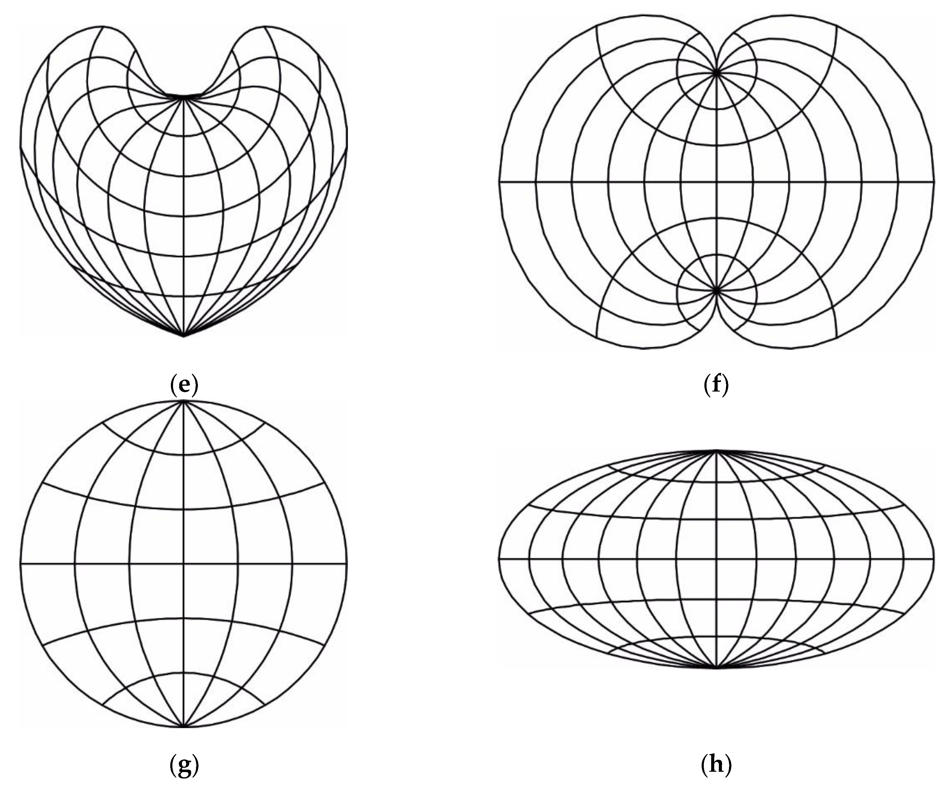
• Pseudocylindrical projections are projections in which pseudomeridians are represented by curves symmetrical with respect to the middle pseudomeridian mapped as a straight line and pseudoparallels as mutually parallel straight lines perpendicular to the image of the central pseudomeridian (Figure 6d).
• Pseudoconic projections are projections in which pseudomeridians are represented by curves symmetric with respect to the middle pseudomeridian mapped as a straight line and pseudoparallels as arcs of concentric circles (Figure 6e).
• Polyconic projections are projections in which pseudomeridians are mapped as curves symmetric with respect to the central pseudomeridian which is mapped as a straight line, and pseudoparallels are mapped as eccentric circles whose centers are on the central pseudomeridian (Figure 6f).
• Circular projections are projections in which pseudomeridians are mapped as arcs of circles symmetrical in relation to the central pseudomeridian which is mapped as a straight line, and pseudoparallels are mapped as arcs of circles whose centers are on the central pseudomeridian (Figure 6g).
• Other projections are projections in which pseudomeridians and pseudoparallels are mapped as more complex curves (Figure 6h).

2.3. Classification of Projections According to the Aspect of Projection

The classification of projections according to the position of the axis of projection in relation to the axis of rotation of the sphere is applied primarily to the mapping of the sphere. Snyder [40] (p. 29) wrote: “While it is fairly straightforward to apply a suitable transformation to the sphere, transformation is much more difficult on the ellipsoid because of the constantly changing curvature. Transformation has been applied to the ellipsoid, however, in important cases under certain limiting conditions.” There is another possibility to map the ellipsoid to a sphere and then the sphere to a plane. In this case, this classification also applies to ellipsoid mapping.

The straight line passing through the poles of the pseudograticule is the axis of projection. The position of the axis of the projection in relation to the axis of rotation of the sphere parameterized by geographical parameterization is called the aspect of the projection. The aspect can be normal, transverse or oblique.

• The normal aspect is the aspect in which the axis of projection coincides with the axis of the sphere, and the pseudograticule coincides with the graticule (Figure 7a).
• The transverse aspect is the aspect in which the axis of projection is perpendicular to the axis of the sphere (Figure 7b).
• The oblique aspect is an aspect that is neither normal nor transverse (Figure 7c).
• It should be emphasized that instead of the normal, transverse and oblique aspect of map projection, the terms normal, transverse and oblique projection are also used. The pseudograticule is also called in the literature the network of verticals and almucantars, and the image of that network in the projection plane is a normal cartographic network, i.e., a network that has a simpler shape in a given group of projections than any other network [26].

Most often, the aspect of projection is explained on maps of the world, but it should be emphasized that maps of an area, such as maps of North America (Figure 8), can be in all three aspects [43].

3. Conclusions

It is not wise to use intermediate developable surfaces in the interpretation of map projections in general because:

• Most map projections in their definition do not have an auxiliary surface.
• The application of the auxiliary/intermediate developable surface can lead to the wrong conclusion about the distortion distribution—standard parallels (parallels with zero distortion) and secant parallels generally do not coincide.
• It is not recommended to classify map projections based on the developable surfaces because such a classification (1) cannot fit many map projections, (2) implicitly or explicitly gives a high weight to the developable surfaces in the theory of map projection which they do not deserve, (3) misleads that standard parallels and secant parallels are one and the same, which is not true in general, and (4) states the wrong conclusion that there are other developable surfaces (pseudocylinders, ovals) by which pseudocylindrical and other map projections can be defined.
• Cylindrical, conical and azimuthal projections belong to the classification of map projections according to the shape of the graticule in normal aspect projections. In such a classification, naturally enter pseudocylindrical, pseudoconical, polyconic and other projections.

Furthermore, there is no need to use developable surfaces in map projection classification. Map projections can be classified into several classes or groups according to different criteria:

• According to kinds of distortions: conformal, equal-area, equidistant and other;
• According to aspect: normal, transversal, oblique;
• According to the form of the graticule in normal aspect: cylindrical, conic, azimuthal, pseudoconic, pseudocylindrical, polyconic, circular and others.

In map projections theory, we do not need conceptuality. We only need reality.

References

- Wikipedia. Map Projection. Available online: https://en.wikipedia.org/wiki/Map_projection (accessed on 6 February 2021).
- Kraak, M.-J.; Roth, R.E.; Ricker, B.; Kagawa, A.; Le Sourd, G. Mapping for a Sustainable World; The United Nations: New York, NY, USA, 2020; Available online: https://unite.un.org/news/mapping-sustainable-world (accessed on 6 February 2021).
- Snyder, J.P. Flattening the Earth: Two Thousand Years of Map Projections; The University of Chicago Press: Chicago, IL, USA; London, UK, 1993. [Google Scholar]
- d’Avezac, M.A.P. Coup d’oeil historique sur la projection des cartes de géographie: Société de Géographie. Bulletin 1863, 5, 257–361; discussion 438–485, Reprinted in Acta Cartographica, 1977, 25, 21–173. [Google Scholar]
- Van Sickle, J. GPS for Land Surveyors, 4th ed.; CRC Press: Boca Raton, FL, USA, 2015. [Google Scholar]
- Van Sickle, J. Map Projection, GEOG 862: GPS and GNSS for Geospatial Professionals, PennState College of Earth and Mineral Sciences, Department of Geography. 2017. Available online: https://www.e-education.psu.edu/geog862/node/1808 (accessed on 5 May 2022).
- Škrlec, D. Geografski Informacijski Sustavi; Script, Faculty of Electrical Engineering and Computing; University of Zagreb: Zagreb, Croatia, 2000. (In Croatian) [Google Scholar]
- Clarke, K.C. Maps & Web Mapping; Kindle, Ed.; Pearson: London, UK, 2015. [Google Scholar]
- Slocum, T.A.; McMaster, R.B.; Kessler, F.C.; Howard, H.H. Thematic Cartography and Geovisualization; Pearson Prentice Hall: London, UK, 2009. [Google Scholar]
- Battersby, S. Map Projections. In The Geographic Information Science & Technology Body of Knowledge, 2nd Quarter 2017 ed.; Wilson, J.P., Ed.; USGIS: Ithaca, NY, USA, 2017. Available online: https://gistbok.ucgis.org/bok-topics/map-projections (accessed on 5 May 2022).
- ESRI. GIS Dictionary. Available online: https://support.esri.com/en/other-resources/gis-dictionary (accessed on 14 March 2022).
- Bolstad, P. GIS Fundamentals: A First Text on Geographic Information Systems, 6th ed.; XanEdu: Ann Arbor, MI, USA, 2019. [Google Scholar]
- Lambert, J.H. Part III, Section 6: Anmerkungen und Zusätze zur Entwerfung der Land- und Himmelscharten. In Beiträge zum Gebrauche der Mathematik und deren Anwendung; Verlag der Buchhandlung der Realschule: Berlin, Germany, 1772; Translated into English and introduced by W. R. Tobler as Notes and comments on the composition of terrestrial and celestial maps: Ann Arbor, Univ. Michigan, 1972, Mich. Geographical Publication no. 8, 125 p. Also reprinted in German, 1894, Ostwald’s Klassiker der Exakten Wissenschaften, no. 54: Leipzig, Wilhelm Engelmann, with editing by Albert Wangerin. [Google Scholar]
- Euler, L. De Repraesentatione Superficiei Sphaericae Super Plano; Academia Scientiarum Imperialis Petropolitanae: St. Petersburg, Russia, 1777; pp. 107–132, Latin. Translated into German as one of Drei Abhandlungen über Kartenprojection, in Ostwald’s Klassiker der Exakten Wissenschaften, no. 93: Leipzig, Wilhelm Engelmann, 1898, with editing by Albert Wangerin, pp. 3–37. [Google Scholar]
- De Lagrange, J.L. Sur la Construction des Cartes Géographiques: Nouveaux mémoires de l’Académie Royale des Sciences et Belles-Lettres de Berlin; 1779; pp. 161–210, Also in Oeuvres de Lagrange, 1869: Paris, Gauthier-Villars, v. 4, p. 635-692. Also in German, 1894, as Ueber die Construction geographischer Karten: Ostwald’s Klassiker der Exakten Wissenschaften, no. 55: Leipzig, Wilhelm Engelmann, p. 1-56, with editing by Albert Wangerin, pp. 82–97. [Google Scholar]
- Gauss, C.F. 1825, Allgemeine Auflösung der Aufgabe: Die Theile einer gegebnen Fläche auf einer andern gegebnen Fläche so abzubilden, daß die Abbildung dem Abgebildeten in den kleinsten Theilen ähnlich wird: Preisarbeit der Kopenhagener Akademie 1822. In Schumachers Astronomische Abhandlungen; Altona: Hamburg, Germany, 1825; pp. 5–30, Reprinted, 1894, Ostwald’s Klassiker der Exakten Wissenschaften, no. 55: Leipzig, Wilhelm Engelmann, pp. 57–81, with editing by Albert Wangerin, pp. 97–101. [Google Scholar]
- Tissot, N.A. Die Netzentwürfe Geographischer Karten, German ed.; Ernst Hammer: Stuttgart, Germany, 1887. [Google Scholar]
- Šavrič, B.; Jenny, B.; Jenny, H. Projection Wizard—An Online Map Projection Selection Tool. Cartogr. J. 2016, 53, 177–185. [Google Scholar] [CrossRef]
- Close, C.F.; Clarke, A.R. Map Projections. Encyclopaedia Britannica; Horace Everett Hooper: USA, 1911, 11th ed. Volume 17, pp. 653–663. Available online: https://www.gutenberg.org/files/42638/42638-h/42638-h.htm#ar1 (accessed on 25 May 2021).
- Lee, L.P. The Nomenclature and Classification of Map Projections. Emp. Surv. Rev. 1944, 7, 190–200. [Google Scholar] [CrossRef]
- Lapaine, M. Behrmann Projection. In Proceedings of the 7th International Conference on Cartography and GIS, Sozopol, Bulgaria, 18–23 June 2018; pp. 226–235. [Google Scholar]
- Lapaine, М. Sekushchie paralleli v azimutal’nyh proektsiyah [Secant Parallels in Azimuthal Projections]. Geod. Cartogr. Geod. I Kartogr. 2019, 80, 39–54. (In Russian)/Лапэн М.: Секущие параллели в азимутальных прoекциях // Геoдезия и картoграфия.–2019.–Т. 80.–No. 4.–С. 39–54. [Google Scholar] [CrossRef]
- Lapaine, M.; Menezes, P. Standard, secant and equidistant parallels/Standardne, presječne i ekvidistantne paralele. Kartogr. I Geoinformacije/Cartogr. Geoinf. 2020, 19, 40–62. [Google Scholar] [CrossRef]
- Lapaine, M. Multi Standard-Parallels Azimuthal Projections. In Cartography—Maps Connecting the World; Robbi Sluter, C., Madureira Cruz, C.B., Leal de Menezes, P.M., Eds.; Springer International Publishing: Cham, Switzerland, 2015. [Google Scholar] [CrossRef]
- Lapaine, M. Conic Projections with Three or More Standard Parallels. In Proceedings of the International Cartographic Association, 30th International Cartographic Conference, Florence, Italy, 14–18 December 2021; pp. 1–6. [Google Scholar] [CrossRef]
- Deetz, C.H.; Adams, O.S. Elements of Map Projection with Application to Map and Chart Construction; U. S. Coast and Geodetic Survey Special Publication 68: Washington, DC, USA, 1934.
- Bugayevskiy, L.M.; Snyder, J.P. Map Projections—A Reference Manual; Taylor & Francis: London, UK, 1995. [Google Scholar]
- Bugayevskiy, L.M. Matematicheskaya Kartografija; Zlatoust: Moscow, Russian, 1998. [Google Scholar]
- Kessler, F.C.; Battersby, S.E. Working with Map Projections; CRC Press; CRFC Press, Taylor & Francis Group: Boca Raton, FL, USA, 2019. [Google Scholar]
- Maurer, H. Ebene Kugelbilder. Ein Linnésches System der Kartenentwürfe. In Petermanns Mitteilungen, Ergänzungsheft; Jusus Perthes: Gota, Germany, 1935; p. 221. [Google Scholar]
- Urmayev, N.A. Matematicheskaja Kartografija; Izdatel’stvo Vojennoinzhenernoj Akademii: Moscow, Russia, 1941. [Google Scholar]
- Kavrayskiy, V.V. Izabranie Trudy, Tom II: Matematicheskaja Kartografija, Vyp. 1. Obshchaja Teorija Kartograficheskih Projekcij; Izdanie Nachalnika Upravlenija Gidrograficheskoj Sluzhbi Voeno-Morskoj Akademii: St. Petersburg, Russia, 1958. [Google Scholar]
- Tobler, W.R. A classification of map projections: Association of American Geographers. Annals 1962, 52, 167–175. [Google Scholar]
- Solov’ev, M.D. Matematicheskaja Kartografija. Izdatel’stvo Nedra: Moskva, Russia, 1969. [Google Scholar]
- Richardus, P.; Adler, R.K. Map Projections for Geodesists, Cartographers and Geographers; North Holland Publishing: Amsterdam, The Netherlands, 1972. [Google Scholar]
- Maling, D.H. Coordinate Systems and Map Projections, 2nd ed.Pergamon Press: Oxford, UK, 1992. [Google Scholar]
- Konusova, G.I. O klassifikatsii kartograficheskikh proyektsiy po kharakteru iskazheniy, Izvestiya Vysshikh Uchebnykh Zavedeniy. Geod. I Aerofotos’yemka 1975, 3, 129–134. (In Russian) [Google Scholar]
- Starostin, F.A.; Vakhrameyeva, L.A.; Bugayevskiy, L.M. Obobshchennaya klassifikatsiya kartograficheskikh proyektsiy po vidu izobrazheniya meridianov i paralleley. Izv. Vyss. Uchebnykh Zavedeniy. Geod. I Aerofotos’yemka 1981, 6, 111–116. (In Russian) [Google Scholar]
- Vakhrameyeva, L.A.; Bugayevskiy, L.M.; Kazakova, Z.L. Matematicheskaja Kartografija; Nedra: Moscow, Russia, 1986. [Google Scholar]
- Snyder, J.P. Map Projections—A Working Manual; U.S. Geological Survey Professional Paper 1395; USGS Publications: Washington, DC, USA, 1987. [Google Scholar] [CrossRef]
- Lapaine, M.; Frančula, N. Map projections aspects. Int. J. Cartogr. 2016, 1, 38–58. [Google Scholar] [CrossRef]
- Frančula, N.; Lapaine, M. Auxiliary Surfaces and Aspect of Projection/O pomoćnim plohama i aspektu projekcije. Kartogr. I Geoinformacije/Cartogr. Geoinf. 2018, 17, 84–89. Available online: http://kig.kartografija.hr/index.php/kig/article/view/820 (accessed on 6 February 2021).
- Lapaine, M.; Frančula, N. Map Projections Selection for Mapping Regions. Problemi Regionalnog Razvoja Hrvatske i Susjednih Zemalja/Regional Development Problems in Croatia and Neighboring Countries, Zagreb, 28–30. Studenoga 2002, Zbornik Radova/Proceedings, Hrvatsko Geografsko Društvo, Zagreb 2005, pp. 37–43. Available online: https://www.bib.irb.hr/198985?&rad=198985 (accessed on 5 May 2021).
Publisher’s Note: MDPI stays neutral with regard to jurisdictional claims in published maps and institutional affiliations. |
© 2022 by the authors. Licensee MDPI, Basel, Switzerland. This article is an open access article distributed under the terms and conditions of the Creative Commons Attribution (CC BY) license (https://creativecommons.org/licenses/by/4.0/).
Share and Cite
Lapaine, M.; Frančula, N. Map Projections Classification. Geographies 2022, 2, 274-285. https://doi.org/10.3390/geographies2020019
Lapaine M, Frančula N. Map Projections Classification. Geographies. 2022; 2(2):274-285. https://doi.org/10.3390/geographies2020019
Chicago/Turabian StyleLapaine, Miljenko, and Nedjeljko Frančula. 2022. "Map Projections Classification" Geographies 2, no. 2: 274-285. https://doi.org/10.3390/geographies2020019
APA StyleLapaine, M., & Frančula, N. (2022). Map Projections Classification. Geographies, 2(2), 274-285. https://doi.org/10.3390/geographies2020019