On Finding a Projected Coordinate Reference System

Abstract

The digital age has brought about an explosion in the growth of data, of which data with a geographical component stands out. Proper use of geographical data comes with the need for correct coordinate reference systems (CRSs). They are considered the ultimate binder for interoperability between geospatial data actors and stakeholders. Moreover, CRSs are crucial for the visual and analytical integration of geospatial data from disparate data sources. However, CRSs might be—for numerous reasons—incorrectly assigned or even missing. The result is a time-consuming study of the map, literature, and available resources to ultimately find the alleged right CRS. This study provides a summary of prevailing resources from national mapping agencies of some European countries to address the above problem. Secondly, and most importantly, is the development of an open-source Python-based software package. This software package aims to accurately estimate the best candidate CRS, given a tuple of coordinates at a priori an approximately known location. It is controlled by geocoding the known location and intersecting the resulting coordinate with the bounding box of all CRSs in the EPSG-database. An in-depth review of CRS tools by mapping authorities reveals, in particular, limitations concerning the countries’ spatial areas, in combination with often required know-how of local CRSs. To address these shortcomings, our tool is developed to enable a more generic extraction of CRSs for any given location worldwide. Testing proved successful for 30 different maps, with a grid present on the map and the CRS of the map being included in the EPSG-database.

1. Introduction

It is estimated that in the information age we are in, a staggering 2.5 billion GB of digital data are produced every day [1,2]. Moreover, a substantial amount of these data—without assessing the exact share—is believed to have some sort of geographical component. When it comes to the collection, management, analysis, and visualization of such data with a geographical component, cartographers, geographers, and geomaticians (s.l.) have played a central role up till now. One of the most principal concerns within the world of geographical data is the quality or reliability of the data. The importance of geographical data quality is something that stems from the myriad of developments in the field of geographical information systems (GIS) since the 1980s [3]. While the concept of geographical data quality has been typically referred to as measurement precision, uncertainty, or error, it well surpasses this. Over and above that, geographical data quality has been more and more considered a dichotomy of both external and internal quality [4]. External quality assesses the goodness of fit for user-specific needs [5]. Contrarily, internal data quality is often centered around a quintet of positional accuracy, temporal accuracy, thematic accuracy, logical consistency, and completeness [6].

Along with the above-mentioned five pillars has emerged the use of metadata, typically accompanying geographical datasets with information about the internal quality [7]. In addition to these five pillars, there is also the so-called lineage of a geographical dataset. When we talk about the lineage of a geographical dataset, we are in particular talking about describing the history of records in the dataset, acquisition methods, and references towards a spatial coordinate system amongst others. The importance of spatial reference systems has been stipulated by the INSPIRE guidelines, notably with a view to interoperability. According to INSPIRE, “interoperability represents the possibility to combine spatial data and services from different sources in a consistent way without involving the specific efforts of humans or machines” [8]. Furthermore, INSPIRE mentions—to our interpretation—coordinate reference systems (CRSs) as a concept to provide a harmonized specification for uniquely referencing spatial information. A horizontal CRS can provide the user the horizontal components while a vertical CRS provides the vertical component. A compound CRS provides both horizontal and vertical components. Note that this explanation can appear difficult to a layperson, as a horizontal CRS providing geographical values (lat, long) actually provides a three-dimensional location on the underlying ellipsoid, while a horizontal CRS providing projected coordinates (x,y) is actually providing a two-dimensional solution. This distinction is mentioned since it is essential for further understanding of this work and its limitations. A geographical CRS expresses two coordinates (lat, long) on a reference ellipsoid, which fits the shape of the Earth (or at least a part of the Earth) as well as possible. Since the ellipsoid is by definition a three-dimensional shape, the (lat, long) coordinates define a three-dimensional location on this ellipsoid. For a projected CRS, (x,y) coordinates are determined. These coordinates describe the planimetric components of (a part of) the Earth that is visualized on a flat surface (such as a map). Projected coordinates suffer from distortions, since there is no mathematical way to represent a three-dimensional physical world on a two-dimensional flat surface without introducing distortion. We refer to [9,10,11] for more information concerning map projections and the basic elements that define a CRS.

Linked to this extensive definition of CRS is the development of the EPSG Geodetic Parameter Dataset, further referred to as EPSG, which simplifies the discovery of CRSs utilized all over the world for creating maps and geodata and for identifying geo-position. EPSG stands for “European Petroleum Survey Group” and is frequently used to refer to the registry of CRS parameters originally developed and maintained by this organization since 1985 and publicly accessible since 1993. Since 2005, the dataset has been maintained by the Geomatics Committee of the International Association of Oil and Gas Producers (IAOGP), which describes the dataset as “a collection of definitions of coordinate reference systems and coordinate transformations which may be global, regional, national or local in application” [12]. CRSs are updated twice a year by the IAOGP and systems are described in accordance with the ISO 19,111 standard [13]. Notwithstanding the widespread use of the dataset, it is not recognized as a standard sensu stricto [14].

Despite the numerous efforts that focus on streamlined procedures for describing geographical data quality and obtaining interoperability using well-defined CRS definitions (such as the aforementioned EPSG standardization in international specifications), there are certain issues. These issues tend to lie at the intersection of geography and geomatics and their interdisciplinary application domains (i.e., geology, archaeology, geomorphology). A considerable number of these domain-specific research fields deal with cartographic/geographical data as of today. This yields a first issue, namely, during the acquisition phase of the data in the field (s.l.), knowledge about geographical data quality is often lacking, which in combination with general bad practices, results in the frequent absence of CRS in the metadata. Secondly, there is an abundance of old topographic survey measurements, analogue historical maps, and libraries of cartographic material—an invaluable source of knowledge—which are being digitized nowadays but where information about the initial CRS of the analogue source is missing. Thirdly, indistinctness might occur when the officially used CRS changes from one system to another (e.g., from Lambert 72 to Lambert 2008 in Belgium or from Gauss–Krüger to UTM in Germany). The above-mentioned concerns have also already been stipulated in [3,15,16]. Specifically, this means that scientists are often confronted with cartographic material, provided with toponyms and annotated in coordinates, but with no further information regarding the spatial reference system.

A very specific objective linked to the problem we defined can be formulated as follows: given a tuple of planimetric coordinates, whose location is known in the form of a toponym (i.e., “in Ghent, Belgium”), it should be possible to find the most appropriate CRS. This (technical) communication seeks to remedy this problem of retrieving the appropriate CRS given a known location and a tuple of coordinates through two solutions. The first solution aims to find which tools are already available by national mapping agencies to solve the research problem. The second solution draws upon a technique that we developed ourselves, relying on the open-source EPSG-libraries embedded in PyProj, combined with the mining of toponym information through geocoding, a widely adopted technique in the field of GIS [17]. The section following this introduction is concerned with the methodology used for our study, comprising the two solutions. Next, there is a section on the validation of our developed technique, with a multitude of test cases. The penultimate section covers an in-depth discussion regarding the cases that are worked out in the validation. Finally, the conclusion gives a summary and critique of the findings, while areas for further research are also identified.

2. Materials and Methods

Retrieving the projected CRS on historical maps can be done in several ways. In this methodological section, we report on common methods of looking for national reference systems using national governmental information and tools on the one hand, before elucidating the automated methodology we implemented using open-source tools on the other hand. Several examples are given in this section, with which we attempt to define problems one might experience when using maps of locations unknown to the researcher. While these experiences are by definition subjective and usually individual, we believe the examples aid in understanding the problem and the proposed automated methodology can be beneficial to researchers in all kinds of research fields, especially those not accustomed to the fields of geography, geomatics, and geodesy.

2.1. Common Method Using National Tools

A common method of finding information regarding the CRS of a historical map is by starting the investigation with an analysis of the information and tools shared by governmental agencies (e.g., National Geographic Institute for Belgium, Ordnance Survey for the United Kingdom, Kadaster for The Netherlands). However, for a layperson, finding a responsible governmental agency can be the first challenge. In the case the responsible agency is found and distributes information on national CRSs, one can experience many difficulties with the technical nature of coordinate systems and geodetic transformations.

2.1.1. Germany

In the case of Germany, a web application for the transformation of coordinates can be found on the website of the Bundesamt für Kartographie und Geodäsie (BKG [18]). The availability and user-friendliness of an online web application are highly appreciated by many users.

However, for a layperson, the web app does not help in identifying the CRS of a map. Some more official information on common CRSs for Germany can be retrieved on the website [19]. While the information on this website suffices for the authors of this work to discriminate between most CRSs when given an example of a coordinate pair, it does not allow to make an immediate and clear distinction between some. For example, the German main triangular network Deutsches HauptDreiecksNetz (DHDN, EPSG:4314) is mentioned to be expressed in geographical coordinates. While several Gauss–Krüger projections are in use over the extent of the country, Universal Transverse Mercator (UTM) is also used. To determine the CRS, given a map with unknown CRS coordinates, the search for the solution becomes complicated and allows for errors. Assume an unidentified location on a map with values 3,549,967 m E, 5,804,301 m N; by using the overview of common CRSs, one can deduce that the coordinate is most probably one of the Gauss–Krüger or UTM CRS. By testing the coordinate in the online coordinate transformation tool, it becomes clear the coordinate is expressed in Gauss–Krüger Zone 3 CRS (EPSG:5677) since the Easting is a value not covered by the minima and maxima values of the extents of the adjacent zones. A similar methodology can be used to exclude the UTM system since in civil UTM32 zone U (EPSG:32632), this location becomes 549,871 m E, 5,802,419 m N. If the map indicated that this location is in or near Hannover (Germany), the backward stepwise selection would become easier by looking up coordinates in the different candidate CRS for this location and then comparing values.

2.1.2. The Netherlands

For the Netherlands, the situation is easier compared to Germany. The Netherlands maintains the main triangular network called Rijksdriehoekscoördinaten and the CRS based on Schreiber’s double projection [20]. Aside from the introduction of a shift in the Cartesian coordinates in 1968, bringing the RD-projection (EPSG:28991) to the RD New-projection (EPSG:28992), no other CRSs appear to have been in use officially. Coordinates expressed in both RD and RD New significantly differ, so the distinction between them is relatively easy. The UTM CRS is also used in the Netherlands, but since the differences between the minima and maxima values of the extents of RD and UTM are quite large, immediately discriminating between these two CRSs is possible. It should be noted, however, that the example given for the case of Germany is relevant here as well. The government provides both an API [21] and an executable software tool called PCTrans [22] to convert coordinates.

2.1.3. Belgium

For Belgium, after World War II alone, the possible CRSs are numerous. Belge 1950/Lambert 50 (EPSG:21500), Belge 1972/Lambert 72 (two versions: EPSG:31300 and EPSG:31370), ETRS89/Belgian Lambert 2005 (EPSG:3447), and ETRS89/Belgian Lambert 2008 (EPSG:2812) are found. By investigating the different CRSs, it appears that only the coordinates in the Lambert 2008 CRS are significantly different from the other CRSs because of a shift of about 500 km in both x- and y-directions. All other CRSs have coordinates that resemble a similar order of magnitude. This is not a problem for applications where high accuracies are required but can be misleading when using old maps that call for high accuracy. UTM 31 and 32 are also available for Belgium. National Geographic Institute Belgium provides an offline software tool to transform between CRSs, called cConvert [23].

2.1.4. The United Kingdom

In the United Kingdom (UK), Ordnance Survey (OS) is responsible for the publication of topographic maps. The default CRS used on maps in the UK is a plane coordinate system that is based on a Transverse Mercator projection whose central meridian is situated 2° west of Greenwich, with standard meridians 180 km west and east of the central meridian. The corresponding UTM zones are 29 and 30. One of the advantages of the UK national grid over the global UTM coordinate system is that it eliminates the boundary between the two UTM zones. We refer to [24] for more information concerning the OSGB36^® datum. While the use of grid systems simplifies the interpretation of historical maps with an unknown CRS, we again mention the possible difficulties for a layperson who has to discriminate between CRSs. Ordnance Survey provides an online transformation tool to convert both single and batches of coordinates between ETRS89 and the OSGB36 national grid [25]. Aside from this online tool allowing only a single type of transformation, the offline tool Grid InQuest II is made available [26], allowing transformation between UTM29N (EPSG:25829), UTM30N (EPSG:25830), UTM31N (EPSG:25831), ETRS89 (EPSG:4258 and EPSG:4936), Irish Grid (EPSG:29902), Irish Transverse Mercator Grid (EPSG:2157), and OSGB36 (EPSG:27700). With this abundance of CRSs, each with its different extremum values within their respective extent, finding the applied CRS becomes a labor-intensive task. We note that the United States of America adopted a similar system to the UK called US National Grid [27]. However, other CRSs are also in use, such as the State Plane Coordinate System.

2.1.5. France

For France, the Institut national de l’information géographique et forestière (IGN) is responsible for the maintenance of the geodetic networks and the CRSs used for maps. The website of the Department of Geodesy [28] provides ample information; a list of CRSs in use for France and its territories is given, indicating that for European France alone, 10 CRSs are legally in use: the Lambert Conformal Conic Lambert93 (EPSG:2154) and the 9 zones conformal conic projection system (EPSG:3942-3950) [29]. While IGN strongly recommends using the Lambert93 CRS, maps could be produced using the 9 zones CRSs. UTM zone 30T, 30U, 31T, 31U, 32T, and 32U are also available for European France. The overseas French territories adopt UTM as the default CRS. A coordinate transformation software tool is provided by IGN, distributed through the website and called Circé [30].

2.1.6. Grand Duchy of Luxembourg

Luxembourg maintains the planimetric network Luxemburg Reference Frame (LUREF) and by default uses the Transversal Mercator projection (also known as the Gauss projection). The Administration du Cadastre et de la Topographie provides all necessary information through their website [31]. By solely using the Luxembourg 1930/Gauss CRS (EPSG:2169), and UTM coverage 31U and 32U, the options remain limited. However, given the size of Luxembourg compared to its neighboring countries Belgium, France, and Germany, maps covering parts of Luxembourg might adopt a different CRS. Luxembourg provides an online coordinate transformation tool with limited functionalities between ETRS89 and LUREF geographic or projected coordinates [32].

2.1.7. Concluding Remarks on Using Common National Tools

As made clear with the aforementioned cases, determining the applied CRS of coordinates on a map can be a complicated and time-consuming task due to the lack of user-friendly software tools, ambiguous information for a layperson (especially in border areas), a surplus of possible CRSs, and mathematical challenges. These arguments are supplemented with problems regarding available languages in which information is provided and sometimes complicated organizational structures of government agencies responsible for the dissemination of geographic information and tools. In this research, solutions were found for some western European countries, notably Belgium and its neighboring countries. However, the conclusions and remarks cannot be generalized. For many countries in the world, governments do not have resources at their disposal to develop and maintain information portals and coordinate transformation software tools. When extending the research to the investigation of maps of regions that were historically occupied by other countries, the CRS of historical maps is based on global systems or implementations of the CRS already applied by the occupying country. The EPSG-database is created with many of the aforementioned problems and arguments in mind. In the following sub-section, using the EPSG-database, we try to propose a simple tool automating the manual iterative backwards stepwise selection methodology to determine the CRS of a map.

2.2. A New Method Using an Automated Decision Process Based on Open-Source Tools

In order to obtain the most probable coordinate reference system (CRS) for a series of coordinates at a given location, a methodology was developed using PROJ. The main purpose of PROJ is to transform coordinates from one CRS to another. The library is written in C/C++ and these operations are made possible using the C API. As part of OSGeo, the library is widely used by various open-source spatial software packages, such as QGIS, and its functionality is available via command-line scripting for various operating systems [33].

Much effort is put into the development of binders that allow the implementation of the PROJ library in other languages, such as R or JavaScript. A popular binder for Python that is already supported since Python 2.5 is PyProj [34]. For this project, PyProj 3.3.0 was used in combination with Python 3.9.0. The platform independence of Python allowed us to successfully test the proposed methodology on Windows 10, Centos 7, MacOS 11, and iPadOS 15. Next to PyProj, the method relies on the Requests-, Shapely- and Pandas-library, which are all widely used by the community.

Powerful tools can be developed by combining PROJ with the EPSG-dataset. The EPSG-database consists of a collection of many of the commonly used CRS and is supplemented with related documents on map projections and geodetic datums. The main advantage of using EPSG is the pooling of CRS used all over the world. As shown in the previous sections, this is not the case for national governmental agencies, where information and transformation tools are often limited to the local CRSs.

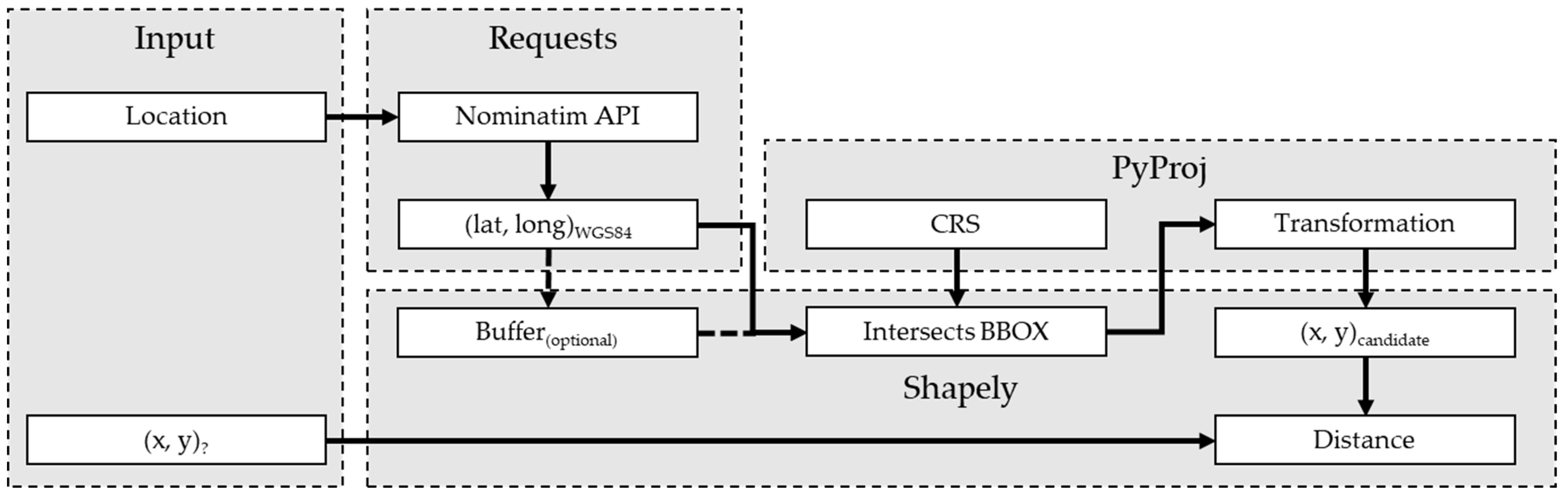
In the software tool we propose, the user submits a series of coordinates, which can either be projected coordinates (x, y) or geographic coordinates (lat, long). A preliminary selection of the CRS (projected or geographic) is based on the nature of the coordinates. The search for the most probable CRS is facilitated by the addition of a geographic locality, which is provided as a string. This string is used to build a simple search query for the Nominatim API [35], resulting in a JSON-object holding multiple possible WGS84 coordinates of the given locality. The quality of these coordinates will depend on the geographic scale of the given locality. These coordinates are iteratively compared with all available CRS-objects in the PROJ-database by finding the intersections of each point with the bounding box of the working area of the CRS, which is given by the EPSG-dataset. For each candidate CRS, the WGS84 coordinate is transformed to a point in this CRS. Perfect correspondence between the transformed coordinates of the given locality and the coordinates with the initially unknown CRS would result in a Euclidean distance equal to zero between these points. All candidate CRSs are stored in a Pandas DataFrame and ordered by this distance. The CRS with the lowest distance is considered the most probable CRS for the initial coordinate. It is important to mention that the distance cannot be used as a parameter to quantitatively evaluate the correspondence between the given and the projected coordinates. In most cases, the accuracy of the coordinate assessment will be hampered by the resolution of the scan, by the scale of the map, and obviously by the interval of the projected grid on the map. Figure 1 presents the methodology of the developed tool, while the code is made available on a GitHub repository [36] (please see the Supplementary Materials).

3. Validation

The methodology was tested on 30 different analogue and scanned historical maps, as well as on contemporary digital maps. To assess the correspondence between the suggested CRS and the true CRS, and thus the quality of the method, information about the CRS should be explicitly mentioned on the map itself, or it should be obtained in the literature. For the evaluation, a distinction was made between four different periods in modern cartography: the contemporary digital era, the analogue post-WWII era, the WWII period, and the pre-WWII era. The presented localities and coordinates were selected randomly as a function of the availability of (online) resources. However, the initial test on the series of contemporary maps was based on the same countries as mentioned in the previous section to indicate the improved level of user-friendliness and the solution to ambiguous situations.

3.1. Validation of Contemporary Topographic Maps from National Mapping Agencies

Based on the results presented in

Table 1. Results of the CRS selection for contemporary topographic maps from national mapping agencies. Three CRSs with the shortest distances are presented: the correct CRS in bold and the wrong suggestions in italics.

Geolocation, Coordinate, Reference	EPSG	Name	Distance (km)
Koblenz, Germany	5677	DHDN/3-degree Gauss-Kruger zone 3 (E-N)	0.35
(3,400,000 m E, 5,581,000 m N)	31467	DHDN/3-degree Gauss-Kruger zone 3 1	0.35
www.geoportal.rlp.de (accessed on 27 February 2022)	5683	DB_REF/3-degree Gauss-Kruger zone 3 (E-N) 2	0.35
Eindhoven, the Netherlands	28992	Amersfoort/RD New	0.50
(161,000 m E, 383,000 m N)	3447	ETRS89/Belgian Lambert 2005	159.61
www.pdok.nl (accessed on 27 February 2022)	31370	BD72/Belgian Lambert 72	160.11
Gent, Belgium	21500	BD50 (Brussels)/Belge Lambert 50 3	0.15
(105,000 m E, 194,000 m N)	31370	BD72/Belgian Lambert 72	0.23
https://ngi.be (accessed on 27 February 2022)	31300	BD72/Belge Lambert 72 4	0.61
Tideswell, United Kingdom	27700	OSGB36/British National Grid	0.85
(415,000 m E, 376,000 m N)	9300	HS2 Survey Grid	257.79
www.ordnancesurvey.co.uk (accessed on 27 February 2022)	9373	MML07 Grid	461.89
Clervaux, Luxembourg	2169	Luxembourg 1930/Gauss	0.53
(70,000 m E, 124,000 m N)	31370	BD72/Belgian Lambert 72	202.78
https://map.geoportail.lu (accessed on 27 February 2022)	21500	BD50 (Brussels)/Belge Lambert 50	202.87
Brest, France	2154	RGF93 v1/Lambert-93	0.70
(146,000 m E, 6,836,000 m N)	9793	RGF93 v2/Lambert-93	0.70
https://ign.fr (accessed on 27 February 2022)	9794	RGF93 v2b/Lambert-93 5	0.70

¹ Given the coordinates as (x, y) = (E, N), the EPSG:31467 cannot be here, as the axis are switched. ² EPSG:5683 is a variant developed by the German national railway company and is not used as an authentic CRS. ³ EPSG:21500 is no longer used on contemporary topographic maps in Belgium. ⁴ EPSG:31300 is a variant of EPSG:31370 with erroneous parameters and should not be used. ⁵ The French national mapping agency has multiple versions of the national CRS. The latest version is considered correct.

, it can be stated that the method performs very well on contemporary CRS and digital cartographic representations. Comparable results were also observed for other map series, such as Austria (tested on Vienna, EPSG:31359, https://bev.gv.at, accessed on 27 February 2022) and Greece (tested on Heraklion, EPSG:2100, https://www.gys.gr, accessed on 27 February 2022), as well as outside Europe, such as the USA (tested on San Francisco, EPSG:6339, https://usgs.gov, accessed on 27 February 2022) and South Africa (tested on Cape Town, EPSG:2048, www.ngi.gov.za, accessed on 27 February 2022).

Caution is required in the interpretation of this table. In the Belgian case, the short distance between the given coordinates and the transformed reference coordinates corresponds with the deprecated Belge Lambert 50 CRS. This means that the minimum distance cannot be considered as the best candidate per se. Furthermore, the distances between the best candidates can be limited, as can be observed for the German and French cases. Variants of the same CRS are represented by different EPSG-codes, where further research is required on the best selection. This problem could be partially solved by limiting the search in the EPSG-database to 2D-projected CRS, not supplemented by a vertical height reference system.

3.2. Validation of Post-WWII and Pre-Digital Maps

Four maps were selected to demonstrate the method, dating between the end of the Second World War and the beginning of digital cartography (

Table 2. Results of the CRS selection for post-WWII and pre-digital maps. Three CRSs with the shortest distances are presented: the correct CRS in bold and the wrong suggestions in italics.

Geolocation, Coordinate, Reference	EPSG	Name	Distance (km)
Joure, The Netherlands	28992	Amersfoort/RD New	0.9
(182,000 m E, 553,000 m N)	5643	ED50/SPBA LCC	351.3
Topographic Survey, 1970	28991	Amersfoort/RD Old	487.8
Moskow, Russia	28407	Pulkovo 1942/Gauss-Kruger zone 7	0.7
(7,414,000 m E, 6,182,000 m N)	20007	Pulkovo 1995/Gauss-Kruger zone 7	0.7
MTD/GSAF, 1987	20907	GSK-2011/Gauss-Kruger zone 7	0.9
Tideswell, United Kingdom	27700	OSGB36/British National Grid	0.8
(415,000 m E, 376,000 m N)	9300	HS2 Survey Grid	257.8
Ordnance Survey, 1961	9373	MML07 Grid	461.9
Kericho, Kenya	32336	WGS 72/UTM zone 36S	0.5
(754,000 m E, 9,959,000 m N)	32736	WGS 84/UTM zone 36S	0.5
British DOS, 1970	21036	Arc 1960/UTM zone 36S	0.7

). In this case, the Russian map has special interest to many modern historical researchers, as this map series offers a detailed and accurate topographic representation of large parts of the post-WWII world [37]. In comparison with the previous overview, equivalent results were obtained and the same caution on the selection of the best CRS candidate based on the distances should be used. It is interesting to mention that the British case is identical to the previous result, notwithstanding the time difference of 61 years, as was expected because of the use of the national grid. The reference to different CRSs in the Dutch case is caused by the fact that this locality is on the northern side of the Netherlands, and outside the bounding box of Belgian CRS.

3.3. Validation of WWII Maps

The Second World War brought many technological developments in modern cartography that were systematically implemented in the following decades [38]. Although large map series were already constructed for many European regions for more than a century (e.g., in Germany [39] or Switzerland [40]), these maps were mainly based on terrestrial observations. Aerial imagery had already been used for mapping during the First World War, but this was more mission-based rather than aiming at the coverage of large areas. The combination of airborne photogrammetry with mature techniques on geodesy and positioning resulted in highly detailed maps, such as the German and Swiss examples in the table below. The French and Egyptian cases are interesting, as they are composed of military services using various data sources, projected on a native CRS (

Table 3. Results of the CRS selection for WWII maps. Three CRSs with the shortest distances are presented: the correct CRS in bold and the wrong suggestions in italics.

Geolocation, Coordinate, Reference	EPSG	Name	Distance (km)
Aachen, Germany	5682	DB_REF/3-degree Gauss-Kruger zone 2 (E-N)	0.3
(2,506,000 m E, 5,626,500 m N)	5676	DHDN/3-degree Gauss-Kruger zone 2 (E-N)	0.3
SOLS, 1939-1945	31466	DHDN/3-degree Gauss-Kruger zone 2	0.3
Brest, France	27561	NTF (Paris)/Lambert Nord France	3.4
(92,000 m E, 99,000 m N)	27571	NTF (Paris)/Lambert zone I	1000.5
ITD, 1943	27572	NTF (Paris)/Lambert zone II	2299.8
Frutigen, Switserland	21781	CH1903/LV03	0.5
(616,000 m E, 160,000 m N)	21780	Bern 1898 (Bern)/LV03C	632.8
Eidg. Landestopographie, 1941	27572	NTF (Paris)/Lambert zone II	2067.3
Cairo, Egypt	22992	Egypt 1907/Red Belt	0.6
(637,000 m E, 815,000 m N)	32236	WGS 72/UTM zone 36N	2528.7
Geographic Section/GS, 1941	32636	WGS 84/UTM zone 36N	2528.7

). This was a frequent practice during WWII in many parts of the world [41].

3.4. Validation of Pre-WWII Maps

Maps predating the Second World War that include a proper grid linked to a CRS with a unique EPSG-code are sparse. In the cases below (

Table 4. Results of the CRS selection for pre-WWII maps. Three CRSs with the shortest distances are presented: the correct CRS in bold and the wrong suggestions in italics.

Geolocation, Coordinate, Reference	EPSG	Name	Distance (km)
Algiers, Algeria	30491	Voirol 1875/Nord Algerie (ancienne)	0.9
(532,000 m E, 387000 m N)	30791	Nord Sahara 1959/Nord Algerie	0.9
Geographic Army Service, 1939	30493	Voirol 1879/Nord Algerie (ancienne)	0.9
Murcia, Spain	2062	Madrid 1870 (Madrid)/Spain LCC	0.7
(824,000 m E,380000 m N)	3034	ETRS89-extended/LCC Europe	2419.9
DGIGC, 1932	3035	ETRS89-extended/LAEA Europe	2854.7
Olomouc, Czech Republic	5513	S-JTSK/Krovak	1.2
(546,000 m E, 1,121,000 m N)	2065	S-JTSK (Ferro)/Krovak	1.2
Military Survey, 1930	8352	S-JTSK [JTSK03]/Krovak	1.2
Konigsberg, Russia	2641	Pulkovo 1995/3-degree Gauss-Kruger zone 7	1.3
(7,468,000 m E, 6,064,000 m N)	2523	Pulkovo 1942/3-degree Gauss-Kruger zone 7	1.3
RfL, 1922	21207	GSK-2011/GSK 3GK zone 7	249.5

), the production of map series continued after WWII ([42] and earlier references). An interesting case here is the 1922 map of Konigsberg, where the proposed CRSs were all implemented after the publication of the map itself. In this case, the correct CRS is selected based the smallest difference between the publication date of the map and the implementation year of the CRS.

3.5. Validation of Maps with Local Geographic CRSs

So far, only projected CRSs have been considered. However, as many geographic CRSs have a unique set of parameters and references to the EPSG-library, they are also included in the PROJ library. A limited test was performed on two historical maps using geographic CRSs, stating that the proposed methodology also applies to these systems (

Table 5. Results of the CRS selection for local geographic CRSs. Three CRSs with the shortest distances are presented: the correct CRS in bold and the wrong suggestions in italics.

Geolocation, Coordinate, Reference	EPSG	Name	Distance (°)
Garoet, Indonesia	4813	Batavia (Jakarta)	0.0048
(1.10° E, −7.12° N)	4211	Batavia	0.1115
Topografische Inrichting, 1920	4238	ID74	0.1115
Heraklion	4815	Greek (Athens)	0.0001
(1.3° E, 35.3° N)	4120	Greek	0.0238
Military Service, 1941	4121	GGRS87	0.0238

). For other examples where coordinates are expressed in a geographic CRS, such as WGS84, NAD27, etc., the most probable CRS could not be selected due to the limited deviations between the various systems.

4. Discussion

Although a series of candidate CRSs is presented in many cases, attentiveness is required in the interpretation of the results. The difference between candidate CRSs might be limited due to small differences in the parameter definition of the system (e.g., Gauss–Krüger variants or projections based on WGS72 or WGS84, or UTM coordinates based on the Hayford ellipsoid or the GRS80-ellipsoid). In this case, a literature study is required to obtain the correct CRS. For the latter, evaluation of the coordinates against the publication date of the source map and the CRS is also helpful, which might be an interesting feature to add to a future release of this tool. Some tested maps did not result in any appropriate suggestions for a CRS. In the following cases, no match was found. For the above example from the Czech Republic, this was easily solved by swapping the (x, y)-coordinates of a given point. In other cases, no successful results were obtained due to:

4.1. Absence of CRS Reference in the EPSG-Database

Since the tool is based on the analysis of all possible CRS using EPSG-codes, registration of CRS in EPSG-database and incorporation in PROJ is required. In various cases, the tool was not able to find the most appropriate CRS for a given coordinate and location. For these cases, the development of new transformation parameters for the EPSG-database is advised. For example:

• Eindhoven, the Netherlands (AMS M831, 26NW, 1943: 443000, 218000): the mentioned Nord de Guerre CRS) is not included in the database [41]);
• Mechelen, Belgium (Karte von Belgien, 23, 1914: 10000, 68000): no CRS is mentioned. As the prime meridian is situated in the middle of the map going through Brussels, the Belgian Bonne-Delambre CRS is assumed, which is not included in the database;
• Waterford, United Kingdom (Deutsche Heereskarte, 29/SO4, 1942: 59630000, 5792000): the map is projected on the Deutscher Heeresgitter [43], which is not included in the database.

4.2. Most probably CRS Results in Unacceptable Translation

• Bucharest, Romania (Directia Topografica Militata, 4040, 1958: 645000, 440000): the assumed CRS, Dealul Piscului 1930/Stereo 33, results in a shift of over 150 km;
• Firenze, Italy (Chief of Engineers, U.S. Army, 106-II, 1943: 579000, 369000): the assumed CRS, Monte Mario/TM Emilia-Romagna, results in a shift of over 400 km.

4.3. Grid Units Are Presented in a Non-metric System

This is a quite common situation for Anglo-Saxon maps, such as the (pre-WWII) maps published by the United States Geological Survey or the British Ordnance Survey. On most of these maps, coordinates are expressed in yards and feet. This also holds for many overseas maps, such as Fuji San, Japan (Chief of Engineers, U.S. Army, 5853-III, 1945, 1371000, 1383000).

4.4. Missing Grid

Although the map under consideration is based on a solid geodetic background, the grid system on the map is missing. This is a customary practice for pre-WWII maps from the Netherlands.

In a number of these cases, one could opt for the use of unambiguously identifiable features on the map itself, such as large constructions or characteristic topographic shapes. However, this is a very time-consuming process and does not always benefit the geometrical quality of the georeferenced map. The quality of the georeferencing—especially when using features on the map—is hampered by various factors, such as the positional accuracy and the scale of the map and mapping errors, as well as scanning resolution and paper distortions [44] To obtain an acceptable result, a large series of ground control points will be required [45]. These factors will influence the georeferencing itself, but the impact on the detection of the most appropriate CRS, as presented in this work, is limited. Hence, especially for large systematic map series, the use of the corners of the map for both georeferencing and CRS determination is advised.

5. Conclusions

Knowledge of the correct CRS is indispensable for the proper use of spatial data and for achieving coherence and consistency of these data. CRSs are frequently unknown for various applications, such as the processing of old land surveying data, georeferencing historical maps, or when information on the CRS is missing in the dataset (e.g., when the PRJ-file is missing in an ESRI Shapefile or when a raster dataset is accompanied by a regular ASCII-encoded world file instead of embedded data about the CRS). A profound study of the map, literature, and resources made available by national mapping agencies are frequently required for recovering the correct CRS.

This paper aims to provide a first overview of existing information and tools provided by national mapping agencies. Furthermore, a new tool based on open-source libraries in Python is presented for the estimation of the best candidate CRS. National mapping agencies maintain country-wide CRSs and provide transformation parameters, and in existing cases, specialized tools for the conversion of coordinates. An overview of these tools is presented in this paper for various European countries (Germany, the Netherlands, Belgium, the United Kingdom, Luxembourg, and France). These tools are limited to their respective territories, and specialized knowledge of CRSs might be required.

To solve the limitations of the spatial extent of these tools, a more generic tool for the extraction of CRSs was developed for any location in the world. The developed tool requires a series of coordinates and a description of the location. The most appropriate CRS is estimated by geocoding the given location and by intersecting the resulting coordinate with the bounding box of all CRSs in the EPSG-database. The geocoding is facilitated by the Nominatim API and the CRS analysis is run using the PyProj-library. Candidate CRSs are selected by the analysis of the distance between the translated reference coordinate and the given coordinate with unknown CRS. The tool was successfully tested for 30 different maps, where a grid is present on the map and the CRS of the map is included in the EPSG-database. Most of these CRSs were projected systems, but some geographic systems were also successfully tested. For these systems, reservation is required on the final selection of the CRS, as the difference between various systems will be limited.

Further research is required on the compatibility of non-EPSG CRSs, availability of the tool, and extension of the overview of information and tools provided by national mapping agencies.

References

- Vopson, M.M. The information catastrophe. AIP Adv. 2020, 10, 085014. [Google Scholar] [CrossRef]
- Zikopoulos, P.; Deroos, D.; Parasuraman, K.; Deutsch, T.; Giles, J.; Corrigan, D. Harness the Power of Big Data The IBM Big Data Platform; McGraw Hill Professional: New York, NY, USA, 2012; ISBN 978-0071808170. [Google Scholar]
- Van Oort, P. Spatial Data Quality: From Description to Application; Wageningen University and Research: Wageningen, The Netherlands, 2006. [Google Scholar]
- Shi, W.; Fisher, P.; Goodchild, M.F. Spatial Data Quality; Taylor & Francis: London, UK, 2002; ISBN 9780367395858. [Google Scholar]
- Dassonville, L.; Vauglin, F.; Jakobsson, A.; Luzet, C. Quality management, data quality and users, metadata for geographical information. In Spatial Data Quality; Taylor & Francis: London, UK, 2002; pp. 202–215. [Google Scholar]
- ISO 19157:2013. Geographic Information—Data Quality; ISO/TC 211: Geneva, Switzerland, 2013.
- Devillers, R.; Bédard, Y.; Jeansoulin, R.; Moulin, B. Towards spatial data quality information analysis tools for experts assessing the fitness for use of spatial data. Int. J. Geogr. Inf. Sci. 2007, 21, 261–282. [Google Scholar] [CrossRef]
- European Commission: Data Specification on Coordinate Reference Systems—Technical Guidelines. Available online: https://inspire.ec.europa.eu/file/1726/download?token=3OGur2Ln (accessed on 22 March 2022).
- Maling, D.H. Coordinate Systems and Map Projections; Pergamon Press: New York, NY, USA, 2013. [Google Scholar]
- Grafarend, E.W.; You, R.-J.; Syffus, R. Map Projections, 2nd ed.; Springer: Berlin/Heidelberg, Germany, 2014; ISBN 978-3-642-36493-8. [Google Scholar]
- Drewes, H. Reference Systems, Reference Frames, and the Geodetic Datum. In Observing our Changing Earth; Sideris, M., Ed.; Springer: Heidelberg, Germany, 2009; pp. 3–9. [Google Scholar]
- EPSG Geodetic Parameter Dataset. Available online: https://epsg.org (accessed on 22 March 2022).
- ISO ISO 19111:2019. Geographic Information—Referencing by Coordinates; ISO/TC 211: Geneva, Switzerland, 2010.
- Nicolai, R.; Simensen, G. The new EPSG geodetic parameter registry. In Proceedings of the 70th European Association of Geoscientists and Engineers Conference and Exhibition 2008: Leveraging Technology (Incorporating SPE EUROPEC 2008), Rome, Italy, 9–12 June 2008; Volume 2, pp. 1136–1140. [Google Scholar]
- Aronoff, S. Geographic Information Systems: A Management Perspective; Taylor & Francis: Abingdon, UK, 1989. [Google Scholar]
- Guptill Stephen, C.; Morrison Joel, L. Elements of Spatial Data Quality; Elsevier: Amsterdam, The Netherlands, 2013. [Google Scholar]
- Goldberg, D.W.; Wilson, J.P.; Knoblock, C.A. From text to geographic coordinates: The current state of geocoding. URISA J. 2007, 19, 33–46. [Google Scholar]
- BKG Germany: Koordinatentransformation. Available online: https://gdz.bkg.bund.de/koordinatentransformation (accessed on 27 February 2022).
- BKG Germany: GDZ-Registry für Koordinatenreferenzsysteme. Available online: http://sg.geodatenzentrum.de/web_registry/crs-gdz/coordinateReferenceSystem/index.html (accessed on 27 February 2022).
- De Bruijne, A.; Van Buren, J.; Kösters, A.; Van Der Marel, H. De Geodetische Referentiestelsels van Nederland: Definitie en Vastlegging van ETRS89, RD en NAP en Hun Onderlinge Relaties; Rijkswaterstaat: Delft, The Netherlands, 2005. [Google Scholar]
- Nederlandse Samenwerking Geodetische Infrastructuur Coördinatentransformatie-API. Available online: https://www.nsgi.nl/coordinatentransformatie-api (accessed on 27 February 2022).
- Ministerie van Defensie The Netherlands: PCTrans. Available online: https://www.defensie.nl/downloads/applicaties/2021/06/30/pctrans5_20210630 (accessed on 27 February 2022).
- NGI Belgium: cConvert. Available online: https://www.ngi.be/website/hulpmiddelen-voor-transformatie-van-coordinaten (accessed on 27 February 2022).
- Greaves, M.; Cruddace, P. The adoption of ETRS89 as the National Mapping System for GB, via a Permanent GPS Network and Definitive Transformation. In Proceedings of the Symposium of the IAG Subcommission for Europe (EUREF), Dubrovnik, Croatia, 30 May–1 June 2002; pp. 193–196. [Google Scholar]
- OS United Kingdom: Coordinate Transformation Tool (OS-Net). Available online: https://www.ordnancesurvey.co.uk/gps/transformation/ (accessed on 27 February 2022).
- OS United Kingdom: OSTN15/OSGM15 Transformation Software. Available online: https://www.ordnancesurvey.co.uk/business-government/tools-support/os-net/transformation (accessed on 27 February 2022).
- Federal Geographic Data Committee (FGDC). United States National Grid (UNSG); FGDC: Reston, VA, USA, 2001. [Google Scholar]
- IGN France: Géodésie. Available online: https://geodesie.ign.fr/ (accessed on 27 February 2022).
- IGN France: Systèmes de Référence de Coordonnées Usités en France. Available online: https://geodesie.ign.fr/contenu/fichiers/documentation/SRCfrance.pdf (accessed on 27 February 2022).
- IGN France: Circé. Available online: https://geodesie.ign.fr/index.php?page=circe (accessed on 27 February 2022).
- ACT Luxembourg: Portail du Cadastre et de la Topographie. Available online: https://act.public.lu/fr.html (accessed on 27 February 2022).
- ACT Luxembourg: Transformation de Coordonnées—Réseaux Géodésiques. GNSS Network. Available online: https://act.public.lu/fr/gps-reseaux/reseaux-geodesiques/trafo-coordonnees.html (accessed on 27 February 2022).
- Kresse, W.; Danko, D.M. Springer Handbook of Geographic Information; Springer: Berlin/Heidelberg, Germany, 2012; ISBN 9783540726807. [Google Scholar]
- PyProj. Available online: https://pyproj4.github.io/pyproj (accessed on 27 February 2022).
- Noninatim API. Available online: https://nominatim.org (accessed on 27 February 2022).
- CRS. Available online: https://github.com/coenist/crs (accessed on 27 February 2022).
- Cruickshank, J.L. The Evolution of Soviet Topographic Maps as Revealed by their Published Supporting Documentation. Cartogr. J. 2021, 1–20. [Google Scholar] [CrossRef]
- Robinson, A.H.; Morrison, J.L.; Muehrcke, P.C. Cartography 1950–2000. Trans. Inst. Br. Geogr. 1977, 2, 18. [Google Scholar] [CrossRef]
- Krüger, G.; Schnadt, J. Die Entwicklung der Geodätischen Grundlagen für die Kartographie und die Kartenwerke 1810–1945; Vermessing: Brandenburg, Germany, 2000; pp. 26–49. [Google Scholar]
- Speich, D. Mountains Made in Switzerland: Facts and Concerns in Nineteenth-Century Cartography. Sci. Context 2009, 22, 387–408. [Google Scholar] [CrossRef] [Green Version]
- Altić, M. Military Cartography of WWII: The British Geographical Section of the General Staff and the US Army Map Service and their Production of the Topographic Map Series of the Balkans (1939–1945). Cartogr. J. 2019, 56, 295–320. [Google Scholar] [CrossRef]
- Čechurová, M.; Veverka, B. Cartometric analysis of the Czechoslovak version of 1:75 000 scale sheets of the Third Military Survey (1918–1956). Acta Geod. Geophys. Hung. 2009, 44, 121–130. [Google Scholar] [CrossRef] [Green Version]
- Buchroithner, M.F.; Pfahlbusch, R. Geodetic grids in authoritative maps—New findings about the origin of the UTM Grid. Cartogr. Geogr. Inf. Sci. 2016, 44, 186–200. [Google Scholar] [CrossRef]
- Timár, G.; Galambos, C.; Kvarteig, S.; Biszak, E.; Baranya, S.; Rüther, N. Coordinate systems and georeference of Norwegian historical topographic maps. In Proceedings of the 12th ICA Conference Digital Approaches to Cartographic Heritage, Venice, Italy, 26–28 April 2017; pp. 146–151. [Google Scholar]
- Biszak, E.; Biszak, S.; Timár, G.; Nagy, D.; Molnár, G. Historical topographic and cadastral maps of Europe in spotlight—Evolution of the MAPIRE map portal. In Proceedings of the 12th ICA Conference Digital Approaches to Cartographic Heritage, Venice, Italy, 26–28 April 2017; pp. 204–208. [Google Scholar]