Article

Geovisualization of Hydrological Flow in Hexagonal Grid Systems

1
Department of Geomatics Engineering, Schulich School of Engineering, University of Calgary, Calgary, AB T2N 1N4, Canada
2
Canada Centre of Mapping and Earth Observation, Natural Resources Canada, Ottawa, ON K1A 0E4, Canada
*
Author to whom correspondence should be addressed.
Geographies 2022, 2(2), 227-244; https://doi.org/10.3390/geographies2020016
Submission received: 20 March 2022 / Revised: 14 April 2022 / Accepted: 26 April 2022 / Published: 29 April 2022
(This article belongs to the Special Issue Geovisualization: Current Trends, Challenges, and Applications)

Abstract

:
Recent research has extended conventional hydrological algorithms into a hexagonal grid and noted that hydrological modeling on a hexagonal mesh grid outperformed that on a rectangular grid. Among the hydrological products, flow routing grids are the base of many other hydrological simulations, such as flow accumulation, watershed delineation, and stream networks. However, most of the previous research adopted the D6 algorithm, which is analogous to the D8 algorithm over a rectangular grid, to produce flow routing. This paper explored another four methods regarding generating flow directions in a hexagonal grid, based on four algorithms of slope aspect computation. We also developed and visualized hexagonal-grid-based hydrological operations, including flow accumulation, watershed delineation, and hydrological indices computation. Experiments were carried out across multiple grid resolutions with various terrain roughness. The results showed that flow direction can vary among different approaches, and the impact of such variation can propagate to flow accumulation, watershed delineation, and hydrological indices production, which was reflected by the cell-wise comparison and visualization. This research is practical for hydrological analysis in hexagonal, hierarchical grids, such as Discrete Global Grid Systems, and the developed operations can be used in flood modeling in the real world.

1. Introduction

Recently, hydrological modeling on hexagonal mesh grids has gained popularity among researchers. Compared to other regular tessellation grids, such as square and triangular meshes, hexagonal cell geometry has noticeable merits in terms of hydrological modeling. First, hexagons eliminate the ambiguity of the cell neighborhood due to its uniform adjacency, and therefore, various weighting schemes and assumptions can be avoided in the cells’ neighborhood. Consequently, hexagonal grids remove the island effect which is an obstacle when modeling watersheds in square grids with both direct and diagonal neighbors [1,2]. Additionally, the cell size is frequently approximated as the flow width in hydrological studies, and this approximation is more sound in hexagonal sampling than rectangular sampling due to its higher compactness, namely the higher area-to-perimeter ratio [3,4].
Research has been carried out to investigate algorithms to compute hydrological geomorphometry parameters in hexagonal meshes. For example, watershed delineation on a hexagonal grid was investigated by Liao, Tesfa, Duan, and Leung [2], where a group of hydrological functions on hexagonal meshes were explored, including flow direction and accumulation, watershed boundary extraction, stream networks, stream order, etc. The study evaluated their algorithm performance by comparing the hexagonal-mesh-based outputs to the square-mesh-based results and observed that the hexagonal mesh grid can contribute to an equivalent and even better performance than traditional methods [2]. The work was further improved in their latest research by adopting hybrid breaching-filling stream burning techniques [5]. In another study, valley lines were modeled based on hexagonal grids, and such a process was shown to maintain a more detailed shape and location accuracy compared to traditional square grids [6]. Wright [4] developed a regular hierarchical surface model where hydrological computation was generalized on hexagonal and triangular grids. The model also offered a pyramid framework to produce coarser values by a scaling function [4].
These existing algorithms can be easily migrated to hexagonal Discrete Global Grid Systems (DGGS), a spatial reference system that hierarchically partitions the Earth’s surface by almost identical hexagonal cells [7]. In fact, researchers have shown increasing interest in managing multi-source geospatial data and developing environmental models to solve real-world problems by using open-sourced DGGS [8,9,10,11]. The proposed analytical operations on hexagonal meshes are useful in the development of hydrological analysis in the DGGS context. In particular, flow routing grids are fundamental in hydrological analysis, which is the basic grid for producing flow accumulation, flow networks, watersheds, etc. However, most of the current research accepted the D6 algorithm, which is analogous to the D8 algorithm over a square grid, to produce flow routing [2,4]. With D6 or D8 algorithms, the flow of a center cell is always routed to the neighboring cell with the lowest elevation [4]. In this study, we explored the other four methods to compute flow direction, essentially following multiple understanding and computations of the slope aspect, in the hexagonal DGGS environment. We evaluated the results by quantitively comparing the consequent flow accumulation and hydrological indices and visualizing the upslope area and watersheds.
The remainder of this paper is arranged as follows: Section 2 shows the quantization process of terrain data as the baseline of this paper. In Section 3, we explain the developed algorithms of hydrological operations in detail. Section 4 introduces three study areas and the experimental environment. Section 5 presents the experiment results. Section 6 discusses the results and points out the directions for future study.

2. Terrain Data Quantization

In this study, the Icosahedral Snyder Equal Area Aperture 3 Hexagonal Grid (ISEA3H) DGGS was adopted as the modeling grid system, and the source terrain data were the Canadian Digital Elevation Model (CDEM), gained from the Canadian Open Government Portal with a resolution of 0.75 arcsec in a south-north direction (https://open.canada.ca/data/en/dataset/7f245e4d-76c2-4caa-951a-45d1d2051333, accessed on 4 August 2021). We followed the quantization method of converting square grid to hexagonal grid elevations proposed by Li, McGrath and Stefanakis [9] who managed to resample elevations at centroid locations of hexagonal cells using bilinear interpolation. Elevation values at the cell centroid locations represent the elevation of a certain hexagonal cell. R library dggridR was used to locate grid cell centroids during this process [12]. Considering the CDEM data were at a resolution of about 400 m2, the finest resolution of the ISEA3H DGGS was chosen as level 24 where the cell area is around 180.6 m2. This was based on the Nyquist–Shannon sampling theorem, which states that the sample rate should be at least double the frequency of the signal component with the highest frequency [13]. By comparing the elevations of ground control points, previous research has shown that the difference between pre-DGGS and post-DGGS elevations was minor at the finest resolution level following the Nyquist–Shannon sampling theorem [9]. Another four successively coarser levels, namely levels 20 to 23, were also examined, where the cell area was 14,628.5, 4876.2, 1625.4, and 541.8 m2, respectively. At coarser levels, we progressively degrade the elevation precision to maintain a rough ratio of horizontal to vertical resolution [9]. During the quantization process, the Quadrilateral 2-Dimensional Integer (Q2DI) indices, which have been implemented in the dggridR library, were also populated for each hexagonal cell. Q2DI is a coordinate-based cell indexing mechanism that is practical in locating neighboring cells around a center cell [14]. To avoid the edge effect, we assigned the edge cells without valid interpolation inputs void elevations.

3. Hydrological Operations

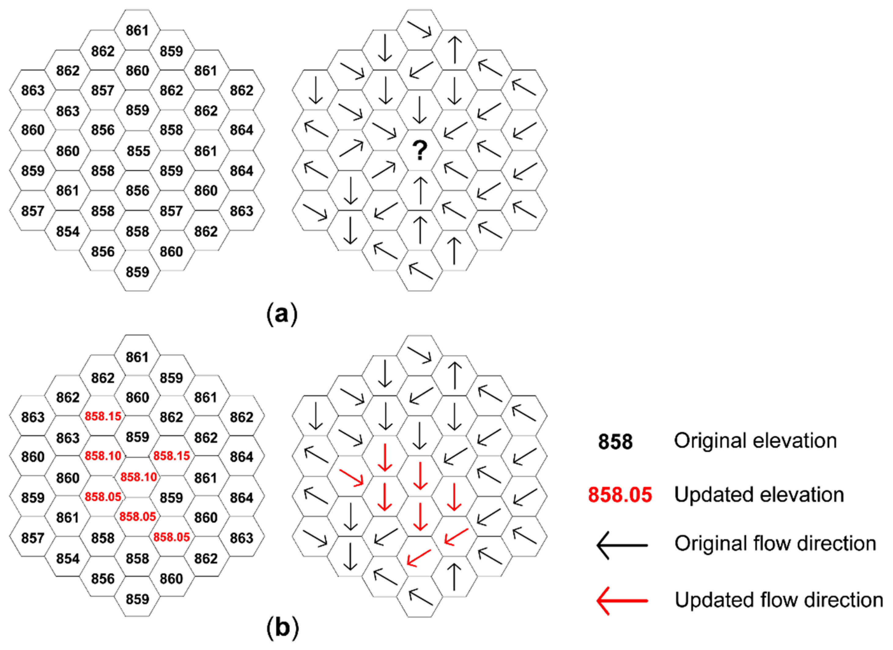
3.1. Pit Filling and Flat Removal
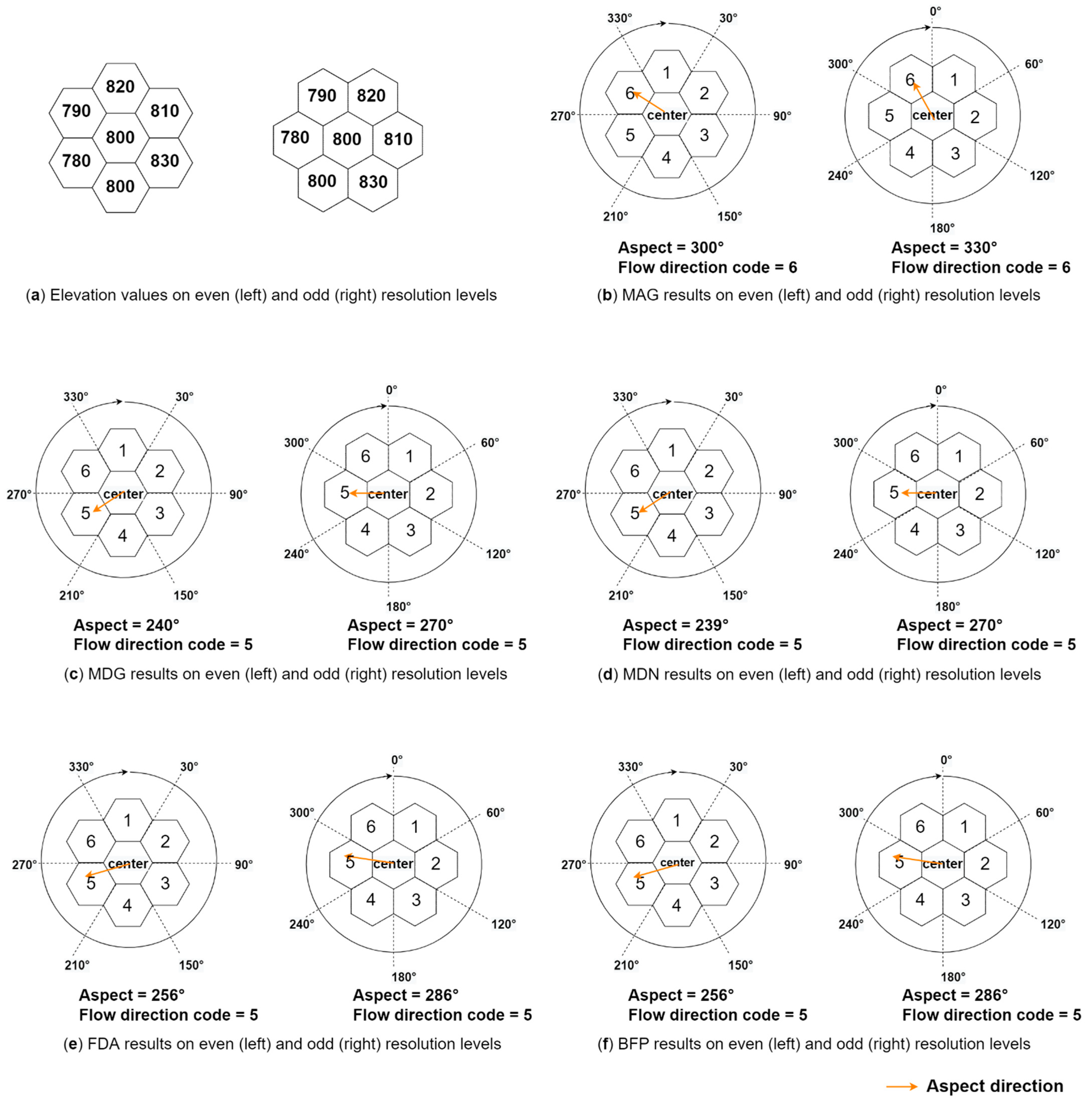
As suggested by previous studies, pits are usually spurious depressions and should be removed during the hydrological analysis [15,16]. In addition, flats are areas of cells with zero slope where flow direction cannot be determined merely with reference to its neighbors [17]. Thus, pits and flats need to be treated before computing flow directions [17]. This study adopted the Priority-flood depression-filling algorithm proposed by Barnes, et al. [18] and adjusted it in the ISEA3H DGGS context to remove pits and flat areas. The algorithm essentially starts from the study area boundary and progressively searches toward the interior, based on the ascending order of elevations in the Priority Queue, to assure that flows cannot be terminated and are along the path where elevations have the smallest changes [18]. This algorithm outperformed other alternatives and showed its feasibility on hexagonal grids [2,5,18]. In our implementation, we applied a small slope (1%) when filling the depression to avoid flat areas, as suggested by Barnes, Lehman and Mulla [18] and Liao, Tesfa, Duan and Leung [2]. Figure 1 shows an example of elevation changes and flow-direction updates after applying the Priority-flood depression-filling algorithm (cell spacing = 5 m). The central cell is considered a pit that does not have a lower neighbor (Figure 1). Flow directions are computed by the D6 algorithm, where the flow of a certain cell is always routed to its lowest neighboring cell [19]. The D6 algorithm is equivalent to the Maximum Downward Gradient (MDG) algorithm in this study, which will be explained more in the following sections. An elevation of 0.05 m is added to form a 1% slope to avoid flat areas after the pit-filling process. More details and step-by-step illustrations can be found in the previous studies [2,18].

3.2. Flow Direction

In this study, flow direction was computed based on five approaches to calculating the slope aspect in the ISEA3H DGGS: Maximum Adjacent Gradient (MAG), Maximum Downward Gradient (MDG), Multiple Downhill Neighbors (MDN), Finite-Difference Algorithm (FDA), and Best-Fit Plane (BFP) methods. The MAG and MDG methods describe the slope aspect as the direction of the first neighboring cell with the maximum absolute elevation difference or the lowest elevation value scanned clockwise from the north, respectively [20,21]. For the MAG method, if the aspect direction is toward an uphill cell, then its directly opposite direction will be assigned to the center cell as the aspect direction [22]. The MDN method examines all downhill neighbors and uses a ‘mean vector’ to represent the orientation of the ‘mean surface’ [23]. The FDA method calculates the finite difference of elevations, and the slope aspect is computed by combining partial derivatives along axes [20,23]. The BFP method fits a local plane surface for each center cell, and the normal vector of the local plane surface is used to calculate the aspect direction [20,23]. Among the five methods, the MAG and MDG lead to six restricted aspect angles, while the other three can result in arbitrary aspect angles ranging from 0 to 360°.
With the aspect angle computed by one of the five methods, the flow direction code 1–6 is assigned to the cell depending on which direction bin it falls in, no matter if the aspect angle is restricted or not (Figure 2). The direction code corresponds to six equally divided direction bins clockwise from north. Because a relative 30° shift of the hexagonal grids’ orientation exists between every two successive resolutions in the ISEA3H DGGS, the specific direction code one cell takes depends on whether it is at an odd-resolution level or an even-resolution level (Figure 2).
Flow direction based on the MDG method on a hexagonal grid is essentially the D6 algorithm, adjusted from the D8 algorithm, applied to rectangular rasters, where the flow always travels along the path of the steepest descent [2,19]. However, flow directions computed by the other four methods, namely MAG, MDN, FDA, and BFP, can potentially cause close loops which will lead to the infinite upstream area [4]. To break the close loops, we adjusted the outlet-breaching methodology used by Jones [16] and extended it into the ISEA3H DGGS context. The specific algorithm has the following steps:
  • Populate all cells with their flow directions according to one of four methods: MAG, MDN, FDA, and BFP.
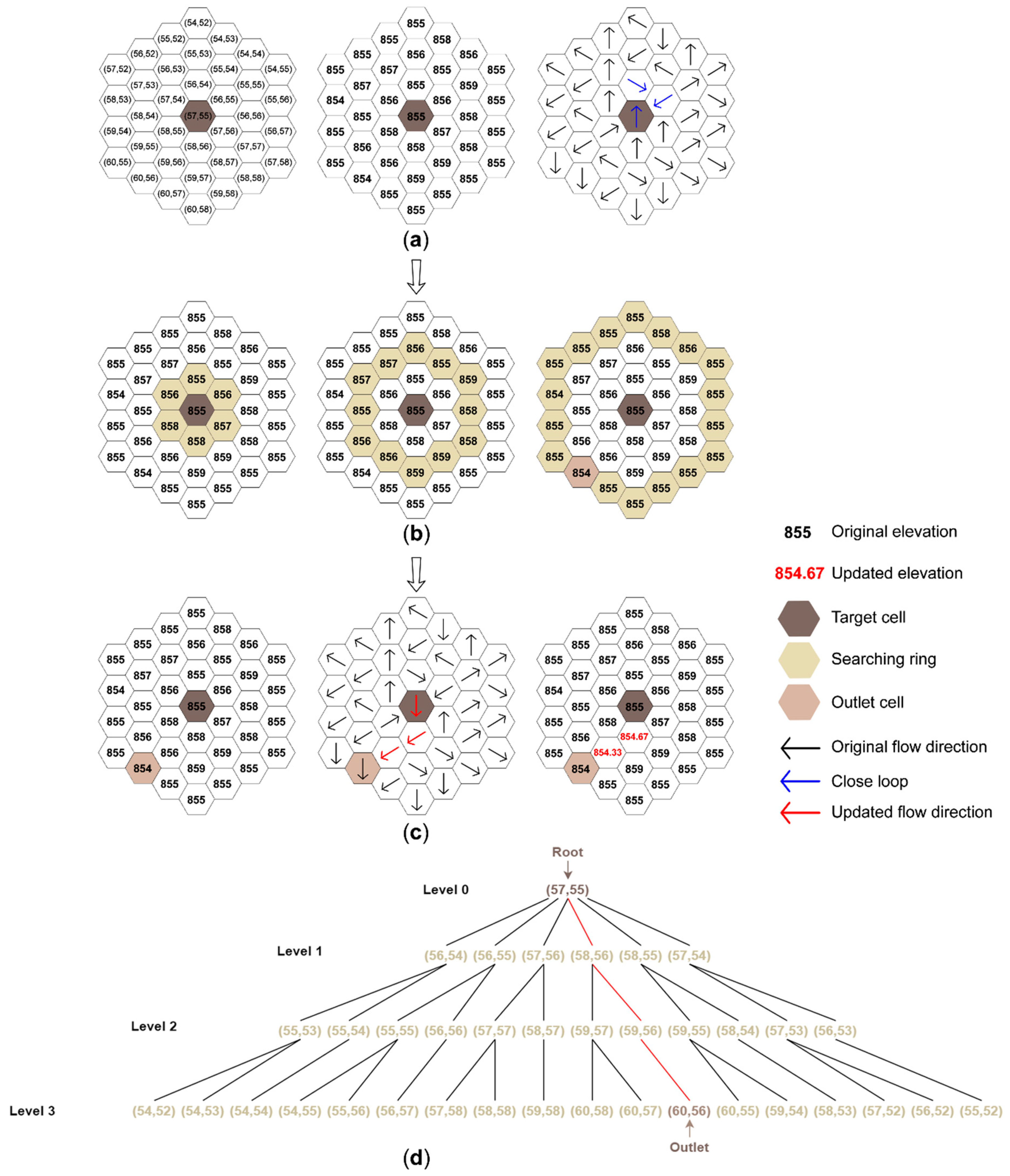
  • Scan all cells following their existing flow directions and record all close loops in a list.
  • Find out the lowest cell in each of the close loops, which is defined as the ‘head’ of the loop. Sort the close loops ascendingly by elevations of their ‘head’ cells.
  • Construct a ‘tree’ for the ‘head’ cell in the first close loop by viewing this cell as the tree root.
  • Deepen the tree by one level by adding the first-ring neighbors as the leaf nodes clockwise from north. Extend each of the leaf nodes by adding their first-ring neighbors as the new leaf nodes clockwise from the north. Duplicated leaf nodes are removed after all neighbors are added. At this point, the tree is deepened to three levels having all of its second-ring neighbors as the new leaf nodes.
  • Continuously deepen the tree until the first candidate outlet is found, where an outlet is defined as an edge cell or a cell with a lower elevation than the tree root. Examine if the candidate outlet flows back to the target ‘head’ cell. If it does, continue to enlarge the search ring until a legit outlet is found.
  • Trace the path from the root cell to the outlet cell and update the flow directions and elevations along the tracing path. New elevations of cells forming the tracing path are an arithmetic sequence with elevations of the root cell and the outlet cell as the first and last term.
  • Remove the broken close loop from the list. If the tracing path passes any cell in any unbroken close loop, remove this close loop from the list as well.
  • Repeat Steps 4–8 until all close loops in the list are broken sequentially.
Figure 3 presents an example of treating a ‘head’ cell in a close loop. Cells’ Q2DI coordinates, elevation values, and flow direction are shown in Figure 3a, where the flow directions result from the MAG method. For example, the cell (58,55) has the highest absolute difference among six neighbors of the cell (57,54), and therefore, the cell (57,54) flows to (56,53) which is in the directly opposite direction of the cell (58,55). At this stage, there should not be any pits and flat areas. As shown in Figure 3a, cells (57,55), (56,54), and (56,55) form a close loop and the ‘head’ cell is (57,55). To break this close loop, a ‘tree’ is constructed and extended for this ‘head’ cell, and a candidate outlet cell (60,56) with a lower elevation of 854 m is found at Level 3 (Figure 3b–d). The outlet is finalized if confirmed not to flow back to the target ‘head’ cell. Then the flow directions and elevations along the tracing path from the ‘head’ cell to the outlet are updated accordingly. Figure 3 shows a case at an even-resolution level, and close loops at an odd-resolution level are broken with the same strategy.

3.3. Flow Accumulation

Flow accumulation, or upslope area, is the total catchment area above a point [15,24]. Flow accumulation algorithms typically count the number of cells contributing flow to the target cells and multiply the count by the cell area [15]. Computing flow accumulation employs a recursive flow climbing algorithm based on the given flow routing grid [15,25]. The algorithm of computing flow accumulation has the following steps [26]:
  • Initialize the inflow count as 0 and upslope count as 1 for all cells.
  • Iterate the cells and determine the inflow count with reference to the existing flow directions for each cell. In other words, the number of cells whose flow direction points to the center cell is saved as the inflow count for the center cell, ranging from 0 to 6.
  • Scan all cells and identify those whose inflow count is 0. For each of the zero-cells, determine which neighboring cell the zero-cell flows into and increase this neighboring cell’s upslope count by the zero-cell’s upslope count.
  • If this neighboring cell’s inflow count is negative and it is not an edge cell, then reset it to 0 and decrease the zero-cell’s inflow count by 1; if not, decrease the inflow count for all cells involved by 1.
  • Repeat Steps 3 and 4 until the inflow count for all cells are negative.
  • The flow accumulation is then calculated as the upslope count multiplying by the cell area.

3.4. Watersheds above Outlets

The watershed over a specific cell is determined by recursively identifying all the cells that contribute to this defined outlet cell according to the flow routing grid. The longitude–latitude coordinate of a potential outlet of interest can be converted to the corresponding cell using the dggridR library. The delineated watershed may differ when the flow routing grids are created by different methods.

3.5. Hydrological Indices

Two hydrological indices are produced, including the Topographic Wetness Index (TWI) and Stream Power Index (SPI). TWI is a geo-morphometric variable used to quantitatively measure the local relief and evaluate the runoff in flood studies, and SPI indicates the potential of the stream to cause erosion and the intensity of surface runoff [24,27]:
TWI = ln ( α tan β )
SPI =   α × tan β
where α is the specific catchment area of a certain cell, and β is the slope gradient in radians at this cell location. The specific catchment area α is defined as the upslope area per unit width of contour and calculated as the upslope area divided by cell spacing [24].

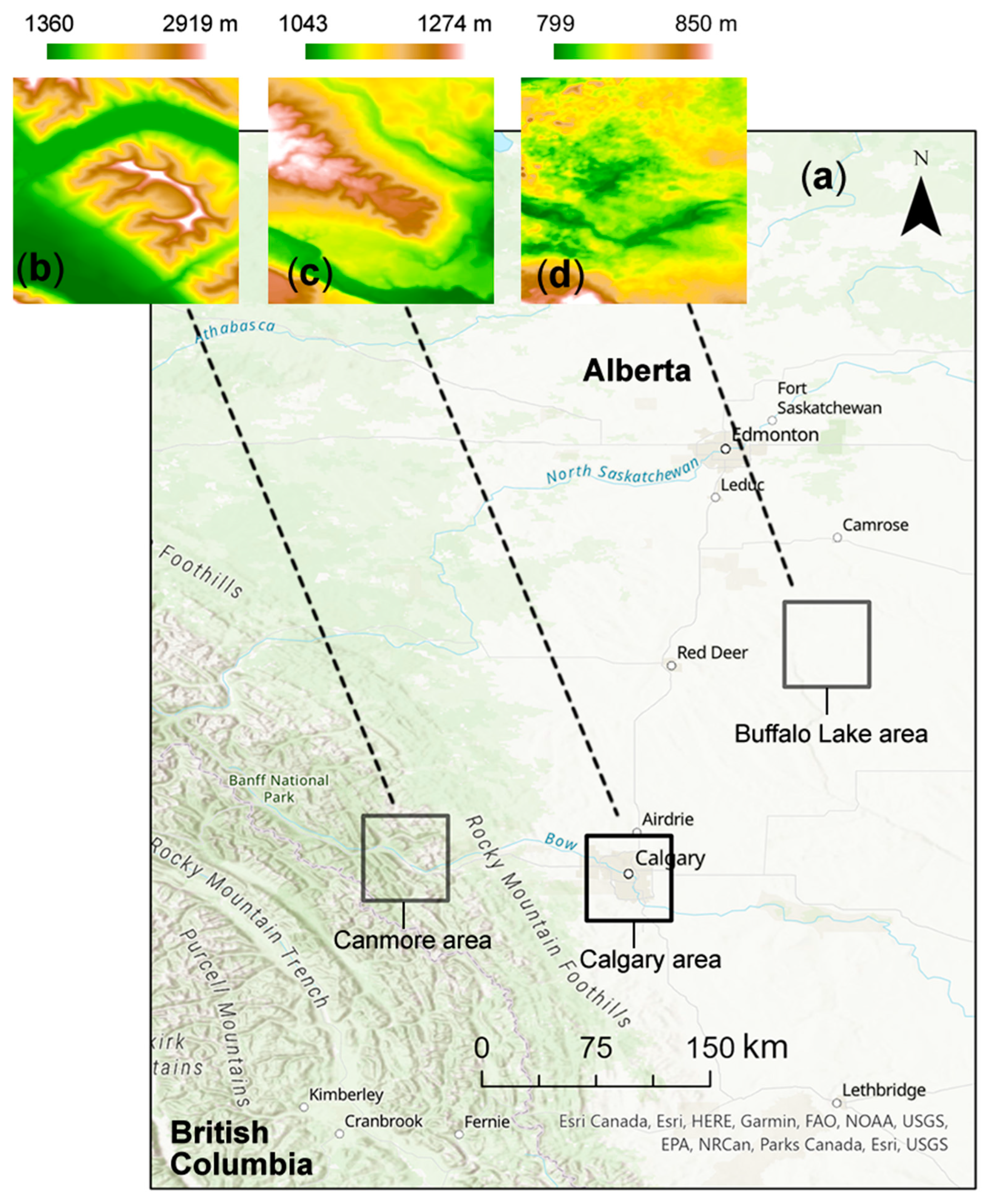
4. Study Area and Experimental Environment

We tested our algorithms over three regions, each around 170 km2 in area (Figure 4). Three study areas locate in Alberta, Canada, and were at different levels of roughness: the Canmore area is the roughest with elevations ranging from 1360 to 2919 m, the Calgary area is moderately rough where elevations range from 1043 to 1274 m, and the Buffalo Lake area has the smoothest terrain with 799 to 850 m elevations. CDEM data were quantized in ISEA3H DGGS at levels 20 to 24 within these study area extents, following the method described in Section 2. All developed functionalities were tested in the ISEA3H DGGS from level 20 to 24, by using the machine with 8 cores, 12 GB memory, and 2× Intel(R) Xeon(R) CPU L5520 @ 2.27GHz.

5. Results

Flow directions computed by five algorithms were not directly and quantitively compared because they were not linear measurements, while the different flow routing grids were reflected by the resulting flow accumulation, watershed delineation, and hydrological indices computation. We pair-wisely compared flow accumulation and hydrological indices derived from multiple flow routing grids and visualized the flow accumulation and watersheds above an outlet at the finest resolution level.

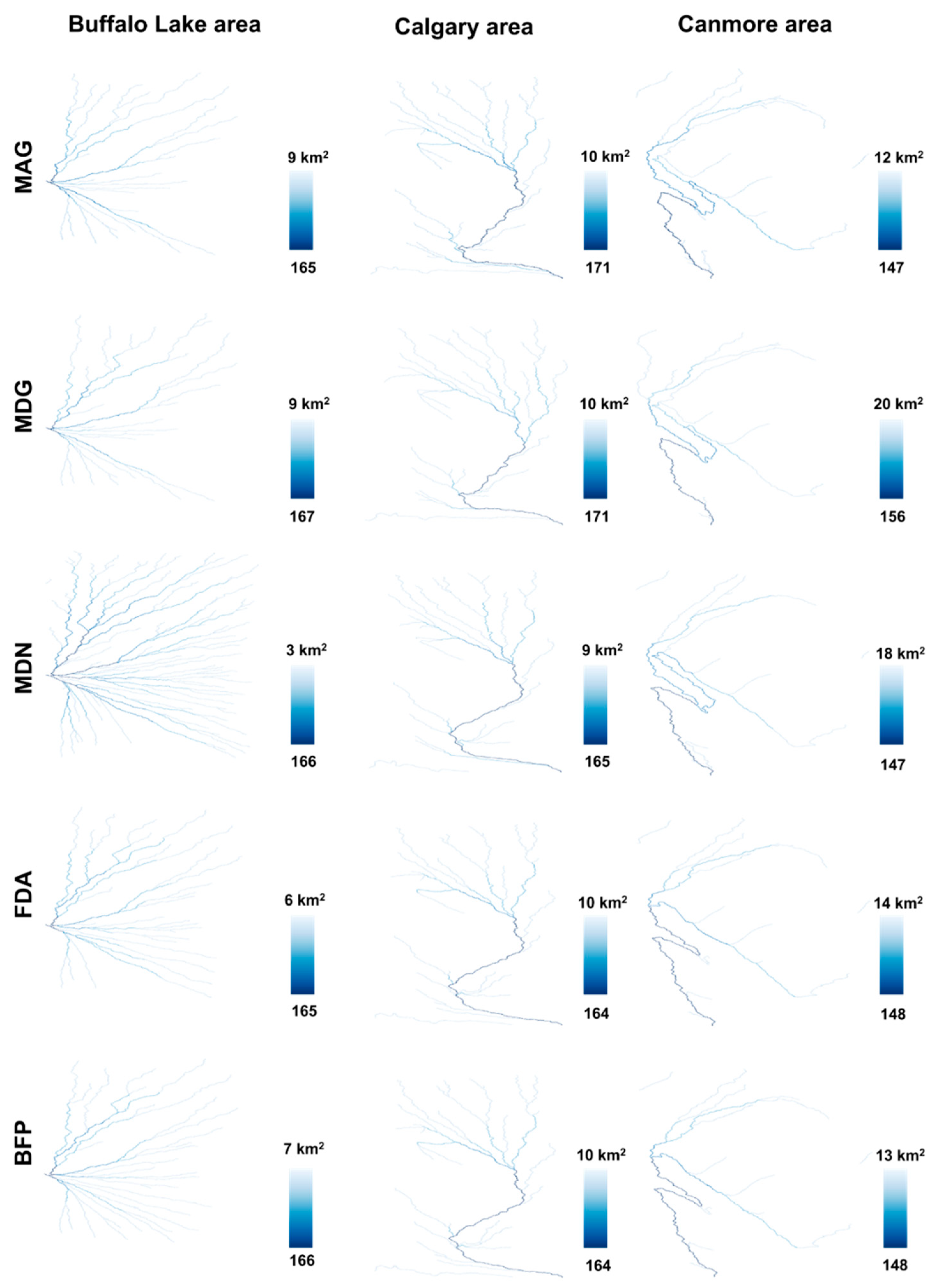
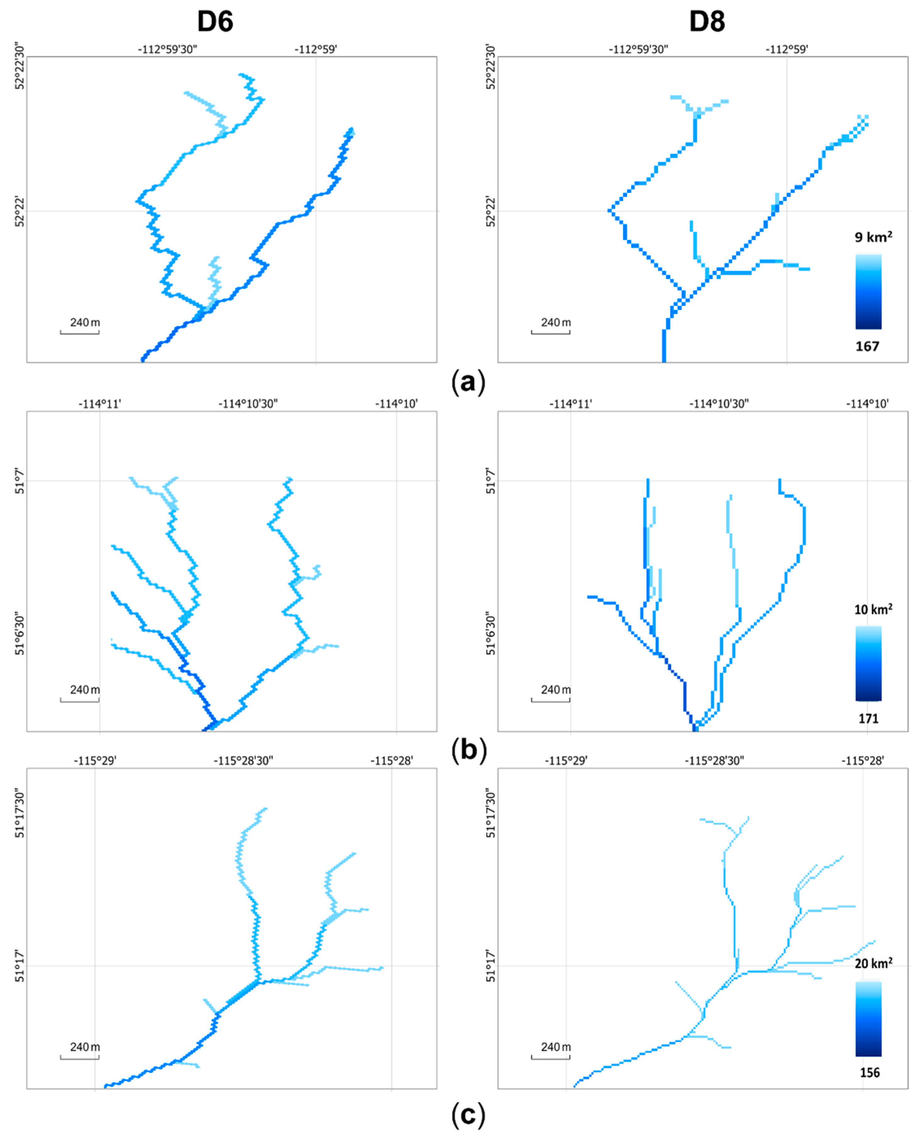
5.1. Flow Accumulation

Based on flow routing grids generated by five algorithms, flow accumulation was recursively computed over all tested areas and resolution levels and compared pair-wisely by Pearson correlation coefficients (r). The results showed that flow accumulation derived from different methods has positive correlation coefficients in all cases, while the coefficient values varied dramatically among resolution levels and study areas (Figure 5). The correlation between the MDG and MDN showed a pattern that r was lower at odd-resolution levels than that at even-resolution levels (Figure 5). It was also noticed that the coefficients between the FDA and BFP methods remained high (r > 0.7) among all resolutions in three areas (Figure 5).
Figure 6 visualizes the flow accumulation generated by five algorithms in three areas at level 24. The maximum flow accumulation of the major outlet within an area was different among various algorithms, most apparently in the Buffalo Lake area which has the smoothest terrain, where the MDN algorithm led to 3 km2 flow accumulation while the MAG and MDG algorithms led to 9 km2 (Figure 6). In the Canmore area, however, the MAG and MDG algorithm contributed to diverse flow routing scenarios, where the maximum flow accumulation was 12 and 20 km2, respectively (Figure 6). We also computed flow directions and flow accumulation among three study areas by Hydrologic Engineering Center’s Hydrologic Modeling System (HEC-HMS) model which adopts the D8 algorithm [29]. Figure 7 visualizes the difference in flow accumulation of a sample branch computed by the HEC-HMS model and the MDG method, namely the D6 algorithm, at the finest resolution.

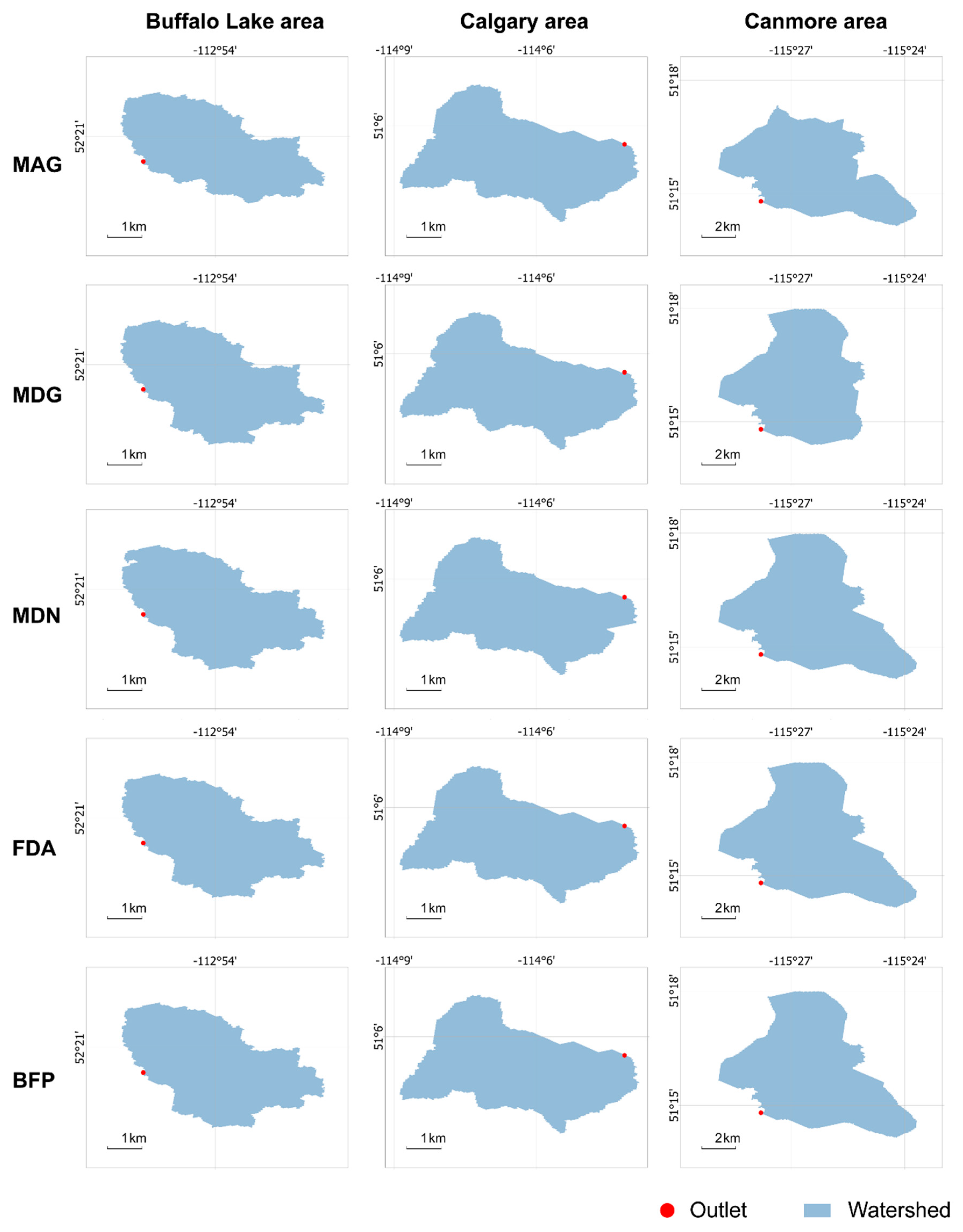
5.2. Watershed Delineation

We defined a random point in each of the three study areas as an example to show the generation of the watershed above it, based on different flow routing grids resulting from multiple slope aspect calculation methods. The longitude–latitude coordinates of the defined outlets are (112.92°W, 52.34°N), (114.06°W, 51.09°N), and (115.46°W, 51.25°N) in the Buffalo Lake, Calgary, and Canmore areas, respectively. The visualization of the watersheds above the defined outlets at level 24 is shown in Figure 8. According to the visualization, created watersheds by the MAG and MDG algorithms in the Canmore area were evidently different from the watersheds created by the other three algorithms (Figure 8). Nonetheless, watersheds based on various flow routing grids in the Buffalo Lake and Calgary areas showed slight differences (Figure 8).

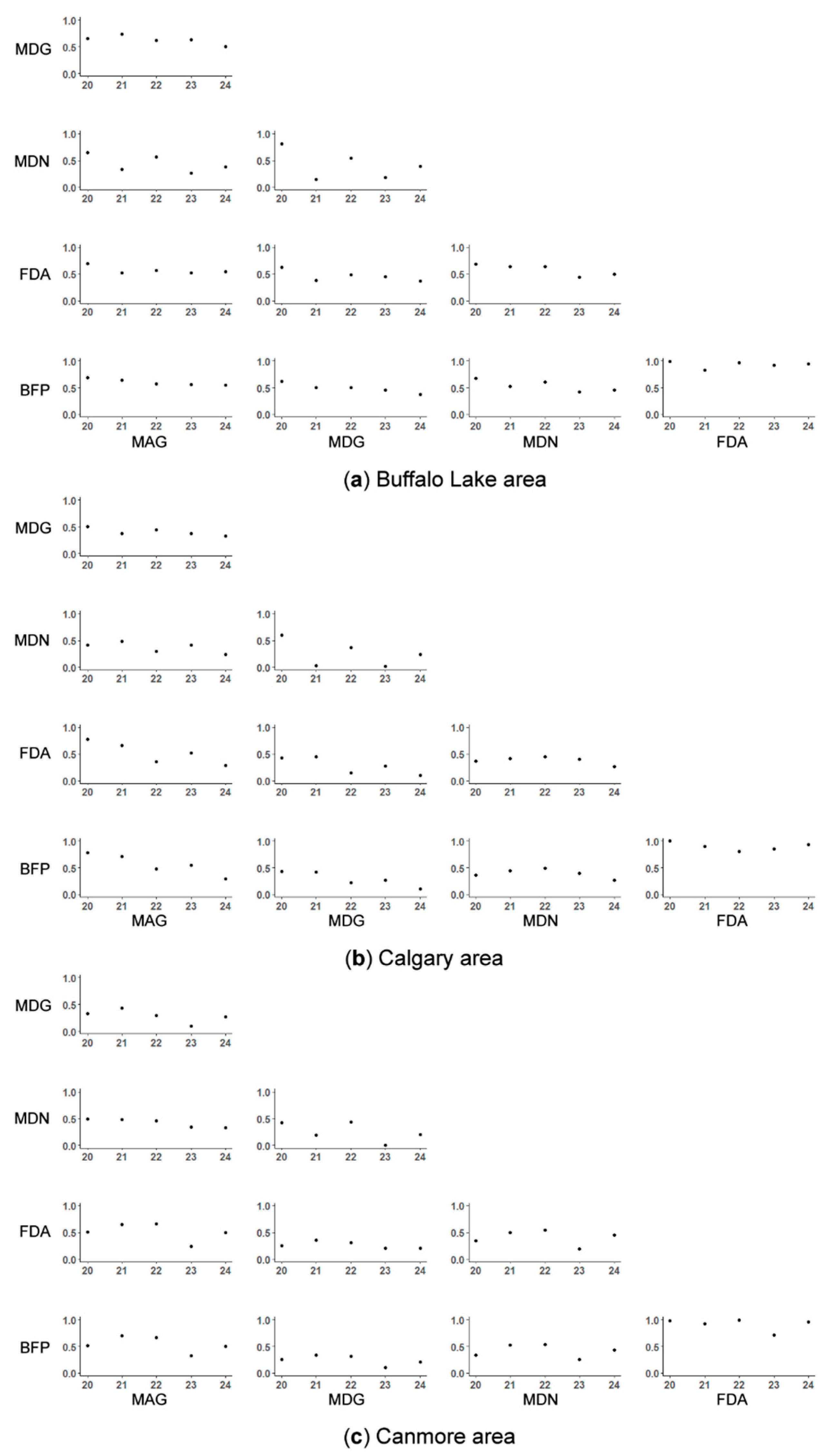
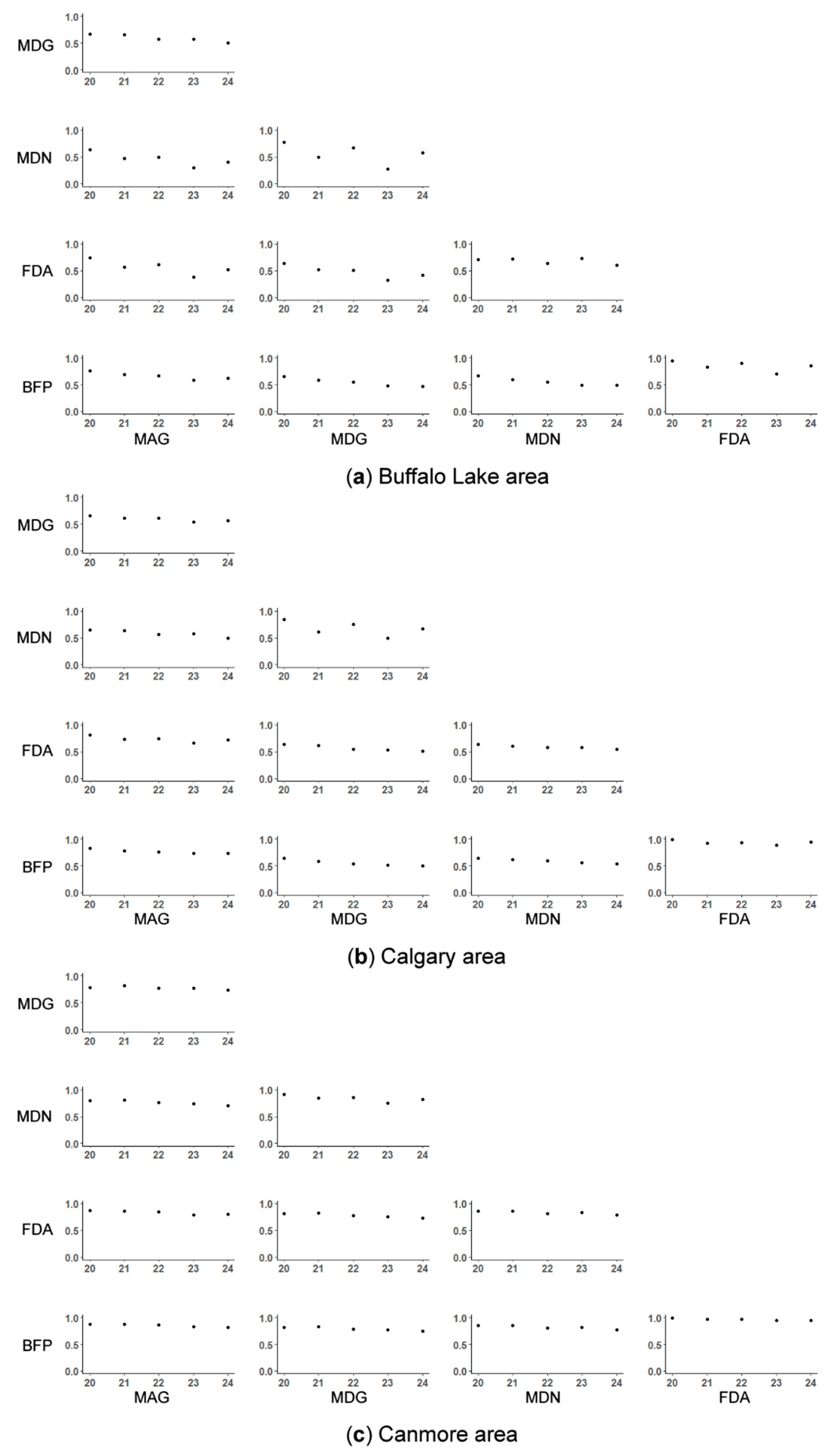
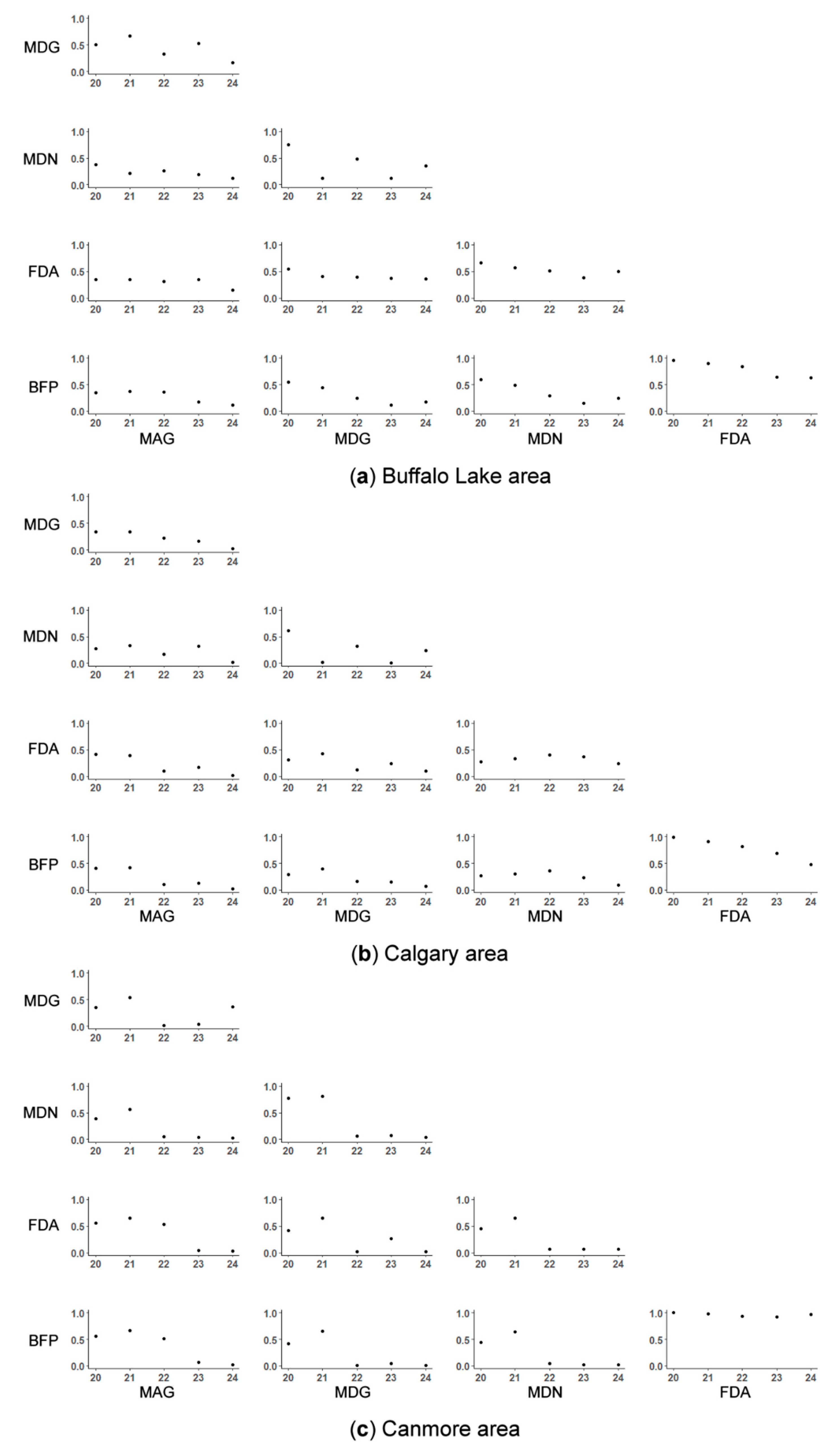
5.3. Hydrological Indices

The Pearson correlation coefficients (r) comparing the TWI values resulting from different slope algorithms were greater than 0.7 in the Canmore area, and greater than 0.5 in the Calgary area, across all resolution levels (Figure 9b,c). The correlation coefficients (r) were relatively lower in the Buffalo Lake area, ranging from 0.3 to 0.9 across the levels (Figure 9a). A high positive correlation (r > 0.7) was observed between the FDA and BFP methods in all study areas (Figure 9). The SPI values derived from different slope aspect algorithms were diverse across resolution levels, which was reflected by highly varied coefficient values without a clear pattern in most cases (Figure 10), except that r remained high (r > 0.9) between the FDA and BFP algorithms in the Canmore area (Figure 10c).

6. Discussion

6.1. Comparison between Flow Routing Methods

The correlation of flow accumulation among five methods differed a lot at multiple granularities in three areas, which reflected that the slope aspect and caused flow routing grids can highly vary depending on the modeling resolution and study area. These uncertainties propagated to the computation of TWI and SPI. Nonetheless, it was observed that the FDA and BFP methods led to highly correlated flow accumulation, TWI, and SPI, in most cases of various modeling resolutions and study areas. This aligned with the conclusion on square grids where the slope and aspect values obtained by the third-order finite-difference algorithm without a weighting factor on eight neighboring cells were the same as those for a least-square linear surface fit to these eight neighboring cells [26]. Among five algorithms used in computing flow directions, the MDG, namely the D6 algorithm, is recommended, because it can avoid close loops after pit-filling processes [2,19,30]. Although we proposed an algorithm to break close loops, it took extra computation time, especially over large areas.
Although without a clear relationship, the differences between calculated flow accumulation and SPI caused by different algorithms, reflected by their pair-wise correlation coefficients, also depended on the resolution level. Such differences in slope gradient and TWI had less sensitivity to resolution, where the correlation coefficients generally remained at the same level across the resolutions.

6.2. Geovisualization in Hexagonal Discrete Global Grids

In this paper, geovisualization was used to convey differences in flow accumulation and watersheds delineation resulting from multiple methods of flow routing production. In terms of geovisualization, DGGS can avoid deformation of the content given that DGGS cells are almost uniform in size and shape at each resolution level [7]. Although geospatial objects in a DGGS need to be projected to be displayed, the expressed geospatial information does not depend on the chosen projection [31]. However, the current visualization of geospatial data modeled in a DGGS relies on existing approaches to display vector or raster data. In this study, modeled geospatial data in the hexagonal DGGS were exported to Esri shapefile to be visualized. Other examples of DGGS visualization include the linkage to PostgreSQL or Leaflet to enable geovisualization in static maps or interactive web maps, respectively [32,33,34]. Some remaining challenges of visualizing massive data modeled in a DGGS at fine resolutions are, for instance, data I/O, data interoperation, and data rendering [35].

6.3. Study Impact and Future Work

The outcome of this paper is useful for hydrological analysis in hexagonal grids, and the developed operations can be generalized in hexagonal DGGS with various aperture, for example, aperture 3, 4, or 7. In previous research, Chaudhuri, Gray and Robertson [10] managed to implement a height above nearest drainage (HAND) model in a hexagonal DGGS platform, while leaving the processes such as determining drainage directions, calculating drainage accumulation, and generating watershed boundaries as GIS-preprocessing based on traditional square Digital Elevation Model (DEM). Hydrological operations developed and compared in this paper are meaningful for flood inundation modeling, for instance, a HAND model, in a pure hexagonal DGGS environment. In addition, flood susceptibility modeling frequently required hydrological parameters as inputs to machine learning models such as a support vector machine, gradient boosting machine, and neural network [36,37,38]. Flood susceptibility predictions based on machine learning methods in hexagonal DGGS can be efficient taking advantage of its discrete nature and power of multi-source data integration [31].
One of the major future study directions is to parallelize the pit-filling and flow accumulation processes. One option is to decompose the dataset into regular tiles and solve each of the tiles independently, then combine adjacent tiles by joining their edges. For example, a linearly scaling algorithm was implemented by Barnes [39], which succeeded in partitioning DEM with regular tiles and parallelizing the Priority-flood depression filling process. Barnes [40] also proposed a parallel algorithm to produce flow accumulation by two sequential MapReduce operations via Message Passing Interface (MPI). On the other hand, the area can be decomposed as sub-basins as the independent units in line with the natural watershed boundaries, so that the stream networks can be connected merely at the watershed outlet points [41]. These parallelization algorithms can be potentially migrated to a hexagonal DGGS environment in the future. Other future directions include allowing flow dispersion when computing flow directions, for example, partitioning and assigning upslope counts to lower neighbors proportionally to their slope gradient [15].

7. Conclusions

This study examined five methods to compute flow directions in an ISEA3H DGGS and developed hydrological operations including flow accumulation, watershed delineation, and hydrological indices computation. An algorithm was also proposed to break the potential close loops created by flow routing. Flow accumulation and hydrological indices resulting from multiple methods were compared quantitatively and visually. It was revealed that the resulting flow routing grids can vary among different approaches, and the impact of such variation can propagate to the follow-up hydrological productions. Among five methods, the D6 algorithm is recommended because it can avoid close loops after pit-filling processes. This research can be a guide for future flood inundation modeling or susceptibility modeling in a pure hexagonal DGGS environment.

Author Contributions

Conceptualization, E.S., H.M. and M.L.; methodology, E.S., H.M. and M.L.; software, M.L.; validation, E.S., H.M. and M.L.; formal analysis, M.L.; investigation, M.L.; resources, E.S. and H.M.; writing—original draft preparation, M.L.; writing—review and editing, E.S., H.M.; visualization, M.L.; supervision, E.S., H.M. All authors have read and agreed to the published version of the manuscript.

Funding

This research was funded by Canadian Natural Sciences and Engineering Research Council (NSERC) Discovery Grant program, grant number RGPIN/03977-2019.

Data Availability Statement

Publicly available datasets were analyzed in this study. This data can be found here: https://open.canada.ca/data/en/dataset/7f245e4d-76c2-4caa-951a-45d1d2051333 (accessed on 4 August 2021).

Acknowledgments

We acknowledge the technical advice from the Research Computing Services at the University of Calgary.

Conflicts of Interest

The authors declare no conflict of interest.

References

  1. Johnston, C.M.; Dewald, T.G.; Bondelid, T.R.; Worstell, B.B.; McKay, L.D.; Rea, A.; Moore, R.B.; Goodall, J.L. Evaluation of Catchment Delineation Methods for the Medium-Resolution National Hydrography Dataset; Scientific Investigations Report 2009–5233; U.S. Department of the Interior, U.S. Geological Survey: Reston, VA, USA, 2009.
  2. Liao, C.; Tesfa, T.; Duan, Z.; Leung, L.R. Watershed delineation on a hexagonal mesh grid. Environ. Model. Softw. 2020, 128, 104702. [Google Scholar] [CrossRef]
  3. Gallant, J.C.; Hutchinson, M.F. A differential equation for specific catchment area. Water Resour. Res. 2011, 47, W05535. [Google Scholar] [CrossRef] [Green Version]
  4. Wright, J.W. Regular Hierarchical Surface Models: A Conceptual Model of Scale Variation in a GIS and its Application to Hydrological Geomorphometry. Ph.D. Thesis, University of Otago, Dunedin, Otago, New Zealand, August 2017. [Google Scholar]
  5. Liao, C.; Zhou, T.; Xu, D.; Barnes, R.; Bisht, G.; Li, H.Y.; Tan, Z.; Tesfa, T.; Duan, Z.; Engwirda, D.; et al. Advances in hexagon mesh-based flow direction modeling. Adv. Water Resour. 2022, 160, 104099. [Google Scholar] [CrossRef]
  6. Wang, L.; Ai, T.; Shen, Y.; Li, J. The isotropic organization of DEM structure and extraction of valley lines using hexagonal grid. Trans. GIS 2020, 24, 483–507. [Google Scholar] [CrossRef]
  7. Alderson, T.; Purss, M.; Du, X.; Mahdavi-Amiri, A.; Samavati, F. Digital Earth Platforms. In Manual of Digital Earth; Guo, H., Goodchild, M., Annoni, A., Eds.; Springer: Singapore, 2020; pp. 25–54. [Google Scholar]
  8. Hojati, M.; Robertson, C. Integrating Cellular Automata and Discrete Global Grid Systems: A Case Study into Wildfire Modelling. In Proceedings of the 23rd AGILE Conference on Geographic Information Science, Chania, Greece, 16–19 June 2020. [Google Scholar] [CrossRef]
  9. Li, M.; McGrath, H.; Stefanakis, E. Integration of heterogeneous terrain data into Discrete Global Grid Systems. Cartogr. Geogr. Inf. Sci. 2021, 48, 546–564. [Google Scholar] [CrossRef]
  10. Chaudhuri, C.; Gray, A.; Robertson, C. InundatEd-v1.0: A height above nearest drainage (HAND)-based flood risk modeling system using a discrete global grid system. Geosci. Model Dev. 2021, 14, 3295–3315. [Google Scholar] [CrossRef]
  11. Robertson, C.; Chaudhuri, C.; Hojati, M.; Roberts, S.A. An integrated environmental analytics system (IDEAS) based on a DGGS. ISPRS J. Photogramm. Remote Sens. 2020, 162, 214–228. [Google Scholar] [CrossRef]
  12. Barnes, R.; Sahr, K.; Evenden, G.; Johnson, A.; Warmerdam, F. dggridR: Discrete Global Grids for R. R Package Version 2.0.4. Available online: https://github.com/r-barnes/dggridR (accessed on 5 March 2020).
  13. Shannon, C.E. Communication in the Presence of Noise. Proc. IRE 1949, 37, 10–21. [Google Scholar] [CrossRef]
  14. Sahr, K. Location coding on icosahedral aperture 3 hexagon discrete global grids. Comput. Environ. Urban Syst. 2008, 32, 174–187. [Google Scholar] [CrossRef]
  15. Tarboton, D.G. A new method for the determination of flow directions and upslope areas in grid digital elevation models. Water Resour. Res. 1997, 33, 309–319. [Google Scholar] [CrossRef] [Green Version]
  16. Jones, R. Algorithms for using a DEM for mapping catchment areas of stream sediment samples. Comput. Geosci. 2002, 28, 1051–1060. [Google Scholar] [CrossRef]
  17. Kenny, F.; Matthews, B.; Todd, K. Routing overland flow through sinks and flats in interpolated raster terrain surfaces. Comput. Geosci. 2008, 34, 1417–1430. [Google Scholar] [CrossRef]
  18. Barnes, R.; Lehman, C.; Mulla, D. Priority-flood: An optimal depression-filling and watershed-labeling algorithm for digital elevation models. Comput. Geosci. 2014, 62, 117–127. [Google Scholar] [CrossRef] [Green Version]
  19. Wright, J.W.; Moore, A.B.; Leonard, G.H. Flow direction algorithms in a hierarchical hexagonal surface model. J. Spat. Sci. 2014, 59, 333–346. [Google Scholar] [CrossRef] [Green Version]
  20. Travis, M.R. VIEWIT: Computation of Seen Areas, Slope, and Aspect for Land-Use Planning; Department of Agriculture, Forest Service, Pacific Southwest Forest and Range Experiment Station: Albany, CA, USA, 1975; p. 70, Rep. PSW 11.
  21. Shanholtz, V.O.; Desai, C.J.; Zhang, N.; Kleene, J.W.; Metz, C.D.; Flagg, J.M. Hydrologic/water quality modeling in a GIS environment. ASAE 1990, 90, 3033. [Google Scholar]
  22. Skidmore, A.K. A comparison of techniques for calculating gradient and aspect from a gridded digital elevation model. Int. J. Geogr. Inf. Syst. 1989, 3, 323–334. [Google Scholar] [CrossRef]
  23. Hodgson, M.E. Comparison of angles from surface slope/aspect algorithms. Cartogr. Geogr. Inf. Syst. 1998, 25, 173–185. [Google Scholar] [CrossRef]
  24. Moore, I.D.; Grayson, R.B.; Ladson, A.R. Digital terrain modelling: A review of hydrological, geomorphological, and biological applications. Hydrol. Process. 1991, 5, 3–30. [Google Scholar] [CrossRef]
  25. Freeman, T.G. Calculating catchment area with divergent flow based on a regular grid. Comput. Geosci. 1991, 17, 413–422. [Google Scholar] [CrossRef]
  26. Raaflaub, L.D.; Collins, M.J. The effect of error in gridded digital elevation models on the estimation of topographic parameters. Environ. Model. Softw. 2006, 21, 710–732. [Google Scholar] [CrossRef]
  27. Beven, K.J.; Kirkby, M.J. A physically based, variable contributing area model of basin hydrology/Un modèle à base physique de zone d’appel variable de l’hydrologie du bassin versant. Hydrol. Sci. Bull. 1979, 24, 43–69. [Google Scholar] [CrossRef] [Green Version]
  28. NRCan. Canadian Digital Elevation Model, 1945–2011. Available online: https://ftp.maps.canada.ca/pub/nrcan_rncan/elevation/cdem_mnec/ (accessed on 4 August 2021).
  29. HEC. Hydrologic Modeling System v.4.9.0. Available online: https://www.hec.usace.army.mil/software/hec-hms/default.aspx (accessed on 5 April 2022).
  30. Wang, L.; Liu, H. An efficient method for identifying and filling surface depressions in digital elevation models for hydrologic analysis and modelling. Int. J. Geogr. Inf. Sci. 2006, 20, 193–213. [Google Scholar] [CrossRef]
  31. Li, M.; Stefanakis, E. Geospatial operations of discrete global grid systems—A comparison with traditional GIS. J. Geovis. Spat. Anal. 2020, 4, 26. [Google Scholar] [CrossRef]
  32. Leaflet. Leaflet: An Open-Source JavaScript Library for Mobile-Friendly Interactive Maps. Available online: https://leafletjs.com/ (accessed on 10 March 2020).
  33. OpenEAGGR. Open Equal Area Global GRid. Available online: https://github.com/riskaware-ltd/open-eaggr (accessed on 26 November 2019).
  34. PostgreSQL. PostgreSQL: The World’s Most Advanced Open Source Relational Database. Available online: https://www.postgresql.org/ (accessed on 1 April 2022).
  35. Hojati, M.; Robertson, C.; Roberts, S.; Chaudhuri, C. GIScience research challenges for realizing discrete global grid systems as a Digital Earth. Big Earth Data 2022, 1–22, ahead-of-print. [Google Scholar] [CrossRef]
  36. Tehrany, M.S.; Jones, S.; Shabani, F. Identifying the essential flood conditioning factors for flood prone area mapping using machine learning techniques. Catena 2019, 175, 174–192. [Google Scholar] [CrossRef]
  37. Esfandiari, M.; Jabari, S.; McGrath, H.; Coleman, D. Flood mapping using random forest and identifying the essential conditioning factors: A case study in Fredericton, New Brunswick, Canada. ISPRS Ann. Photogramm. Remote Sens. Spat. Inf. Sci. 2020, V-3-2020, 609–615. [Google Scholar] [CrossRef]
  38. McGrath, H.; Gohl, P.N. Accessing the impact of meteorological variables on machine learning flood susceptibility mapping. Remote Sens. 2022, 14, 1656. [Google Scholar] [CrossRef]
  39. Barnes, R. Parallel Priority-Flood depression filling for trillion cell digital elevation models on desktops or clusters. Comput. Geosci. 2016, 96, 56–68. [Google Scholar] [CrossRef] [Green Version]
  40. Barnes, R. Parallel non-divergent flow accumulation for trillion cell digital elevation models on desktops or clusters. Environ. Model. Softw. 2017, 92, 202–212. [Google Scholar] [CrossRef] [Green Version]
  41. Gong, J.; Xie, J. Extraction of drainage networks from large terrain datasets using high throughput computing. Comput. Geosci. 2009, 35, 337–346. [Google Scholar] [CrossRef]
Figure 1. Illustration of elevation changes and flow direction updates after applying the Priority-flood depression-filling algorithm on hexagonal grids (cell spacing = 5 m; [18]): (a) original elevations and flow directions based on the D6 algorithm where the central cell is a pit [19]; (b) elevations and flow direction after pit-filling process where updated elevations and flow directions are marked as red.
Geographies 02 00016 g001
Figure 2. Illustration of flow direction code assignment an even and odd resolution levels based on (b) Maximum Adjacent Gradient (MAG), (c) Maximum Downward Gradient (MDG), (d) Multiple Downhill Neighbors (MDN), (e) Finite-Difference Algorithm (FDA), and (f) Best-Fit Plane (BFP) methods. Elevation values of cells are shown in (a).
Geographies 02 00016 g002
Figure 3. Illustration of the algorithm to break a close loop at an even-resolution level: (a) Coordinates, elevations, and flow directions of a sample group of cells with an existing close loop, where a ‘head’ cell with the lowest elevation within the loop is determined; (b) Search by enlarging rings around the target ‘head’ cell until a candidate outlet is found at the third ring; (c) Examine if the candidate outlet flows back to the target ‘head’ cell, if not, update the flow directions and elevation values along the tracing path; (d) A ‘tree’ structure is constructed during the search process.
Geographies 02 00016 g003
Figure 4. The spatial locations of three study areas (a) in Alberta, Canada, and the rendered elevations [28] in (b) Canmore area, (c) Calgary area, and (d) Buffalo Lake area.
Geographies 02 00016 g004
Figure 5. Correlation matrix of Pearson correlation coefficients of calculated flow accumulation by Maximum Adjacent Gradient (MAG), Maximum Downward Gradient (MDG), Multiple Downhill Neighbors (MDN), Finite-Difference Algorithm (FDA), and Best-Fit Plane (BFP) methods from level 20 to 24 in (a) Buffalo Lake area, (b) Calgary area, and (c) Canmore area (p < 0.0001).
Geographies 02 00016 g005
Figure 6. Visualization of flow accumulation in three study areas at level 24, derived from Maximum Adjacent Gradient (MAG), Maximum Downward Gradient (MDG), Multiple Downhill Neighbors (MDN), Finite-Difference Algorithm (FDA), and Best-Fit Plane (BFP) methods.
Geographies 02 00016 g006
Figure 7. Visualized comparison of a zoom-in sample branch computed by D6 and D8 algorithms at level 24 in (a) Buffalo Lake area, (b) Calgary area, and (c) Canmore area.
Geographies 02 00016 g007
Figure 8. Visualization of the watersheds above a random point in each of three study areas at level 24, derived from Maximum Adjacent Gradient (MAG), Maximum Downward Gradient (MDG), Multiple Downhill Neighbors (MDN), Finite-Difference Algorithm (FDA), and Best-Fit Plane (BFP) methods.
Geographies 02 00016 g008
Figure 9. Correlation matrix of Pearson correlation coefficients of calculated Topographic Wetness Index (TWI) by Maximum Adjacent Gradient (MAG), Maximum Downward Gradient (MDG), Multiple Downhill Neighbors (MDN), Finite-Difference Algorithm (FDA), and Best-Fit Plane (BFP) methods from level 20 to 24 in (a) Buffalo Lake area, (b) Calgary area, and (c) Canmore area (p < 0.0001).
Geographies 02 00016 g009
Figure 10. Correlation matrix of Pearson correlation coefficients of calculated Stream Power Index (SPI) by Maximum Adjacent Gradient (MAG), Maximum Downward Gradient (MDG), Multiple Downhill Neighbors (MDN), Finite-Difference Algorithm (FDA), and Best-Fit Plane (BFP) methods from level 20 to 24 in (a) Buffalo Lake area, (b) Calgary area, and (c) Canmore area (p < 0.0001).
Geographies 02 00016 g010
Publisher’s Note: MDPI stays neutral with regard to jurisdictional claims in published maps and institutional affiliations.

