Article

Spatial Modelling and Geovisualization of House Prices in the Greater Athens Region, Greece

by
Polixeni Iliopoulou
1,* and
Elissavet Feloni
1,2
1
Department of Surveying & Geoinformatics Engineering, Egaleo Park Campus, University of West Attica, Ag. Spyridonos Str., 12243 Athens, Greece
2
Department of Water Resources and Environmental Engineering, School of Civil Engineering, National Technical University of Athens, Heroon Polytechniou 9, 15780 Athens, Greece
*
Author to whom correspondence should be addressed.
Geographies 2022, 2(1), 111-131; https://doi.org/10.3390/geographies2010008
Submission received: 28 December 2021 / Revised: 17 February 2022 / Accepted: 18 February 2022 / Published: 21 February 2022
(This article belongs to the Special Issue Geovisualization: Current Trends, Challenges, and Applications)

Abstract

:
In this article, geovisualization is used for the presentation and interpretation of spatial analysis results concerning several house attributes. For that purpose, point data for houses in the region of Attica, Greece are analyzed. The data concern houses for sale and comprise structural characteristics, such as size, age and floor, as well as locational attributes. Geovisualization of house characteristics is performed employing spatial interpolation techniques, kriging techniques, in particular. Spatial autocorrelation in the data is examined through the calculation of the Moran’s I coefficient, while spatial clusters of houses with similar characteristics are identified using the Getis-Ord Gi* local spatial autocorrelation coefficient. Finally, a model is developed in order to predict house prices according to several structural and locational characteristics. In that respect, a classic hedonic pricing model is constructed, which is consequently developed as a geographically weighted regression (GWR) model in a GIS environment. The results of this model indicate that two characteristics, i.e., size and age, account for most of the variability in house prices in the study region. Since GWR is a local model producing different regression parameters for each observation, it is possible to obtain the spatial distribution of the regression parameters, which indicate the significance of the house characteristics for price determination in different locations in the study area.

Graphical Abstract

1. Introduction

The purpose of this article is to present spatial analysis results and suggest how geovisualization can contribute to their interpretation. For that purpose, spatial data concerning houses for sale in the Attica region, Greece are used. Statistical methods for the visualization of the data are employed instead of thematic cartography methods or deterministic interpolation techniques. Geostatistical methods (kriging analysis) and hot-spot analysis are used to depict statistically significant spatial clustering. In this way, areas within the study region with high and low values of certain variables are identified. In addition, a spatial regression model (Geographically Weighted Regression—GWR) is presented for estimating house prices according to several house characteristics. One main purpose for building up this model is to show ways to visualize the results of regression analysis, since this is important for their interpretation. The model is developed in a geographic information systems (GIS) environment and it is possible to map the importance of the factors influencing house prices in terms of mapping the regression coefficients. The regression coefficients vary over the study region and their geographical distribution can be interpreted according to the characteristics of different areas. In order to build the spatial regression model, a conventional multiple regression model (ordinary least squares–OLS) is the starting point. If the residuals of the OLS model are clustered, there is good chance that the results will be improved by a GWR model.
The data in this study include several characteristics, such as price, size, age and locational attributes. Several characteristics were derived from publicly available webpages, while some locational attributes were calculated through GIS operations. There is great differentiation in prices and house characteristics in the study region, as previous research has suggested [1,2,3]. Apart from the structural characteristics of the houses, such as size, age, condition etc., location is a very important factor for housing prices and geovisualization is necessary in order to explore the spatial variation in prices and the other house characteristics.
Geovisualization of house data is carried out using spatial analysis techniques, which incorporate the statistical properties of spatial data. Thematic maps are the first exploratory step in order to present the spatial variation of house characteristics. For point data, dot maps are common [2], although choropleth maps can be used, because they present clearer spatial patterns [1]. Spatial interpolation techniques, which create surfaces of values for a given characteristic, are also used in some studies for the visualization of house data [4].
Beyond data description, spatial analysis methods can identify spatial clusters of observations sharing similar characteristics, which are also statistically significant. For that purpose, the concept of spatial autocorrelation is important, indicating that observations at small distances from each other will share similar characteristics relative to observations far apart. Spatial autocorrelation is a common characteristic of spatial data; it is obvious for meteorological measurement or air pollution, but it is also observed for house characteristics.
There are indices that measure spatial autocorrelation for s whole region, including all observations, such as the Moran’s I coefficient, and indices that can identify spatial clusters of observations with similar characteristics. These are the indices of local spatial autocorrelation, such as the local Moran’s I and the Getis–Ord Gi* coefficients. In this way, spatial clusters are identified, which are tested with inferential statistics and presented according to their statistical significance [5]. In this study, house characteristics are depicted using geostatistical techniques. Kriging analysis, in particular, is used in order to produce statistical surfaces for selected house characteristics. In order to measure spatial autocorrelation for these variables, the global Moran’s I indicator is calculated, while the Getis–Ord Gi* coefficient is used in order to identify spatial clusters.
Differences in housing prices across geographical regions can be attributed to a large variety of house characteristics, which can be organized in three groups: structural attributes, neighborhood characteristics and locational influences [6,7,8]. Structural attributes describe the physical structure of the property, such as size, age, floor and type of dwelling. Neighborhood characteristics refer to the socioeconomic conditions, such as crime, quality of schools, etc. Locational influences mainly describe proximity to locations of interest, such as parks, recreation areas and transportation [9,10,11,12,13,14].
In order to explore the factors that contribute to property values, hedonic regression is the most common technique [1,6,15]. These are regression models, in which house price is the dependent variable and a set of house characteristics the explanatory factors. Usually, linear regression models are used, however, there are variations, such as the transformations of the dependent and/or the independent variables [16]. On the other hand, several studies employ spatial regression models in order to study the spatial variation of housing prices [1,4,17,18,19,20]. In these models, the relative location of the observations is incorporated in the model, therefore, spatial autocorrelation is accounted for.
The main reason for using spatial regression models is that classic regression models are misspecified due to the presence of spatial autocorrelation and, therefore, the description of the data and the calculation of the regression parameters are not accurate [21,22]. For that same reason, several studies indicate the better fit of the spatial regression models when compared with the classic ones, although this is not the case for all datasets [1,23]. In addition, since spatial regression models capture the spatial variation of house characteristics, it is possible to achieve the more accurate prediction of the dependent variable when entering a smaller number of independent variables.
In this study, first, a classic linear regression model is constructed and the results are examined in terms of problems in the specification of the model resulting from spatial autocorrelation. Since spatial autocorrelation is detected in the error term, it is recommended that a hedonic pricing model is developed in a GIS environment, namely, a geographically weighted regression (GWR) model. This method produces local regression models, allowing spatial variation of the regression coefficients [22]. In this way, it is possible to identify areas where individual regression coefficients, for example, the regression coefficient of the independent variable “size” of the house, indicate a greater or lower impact on house prices.

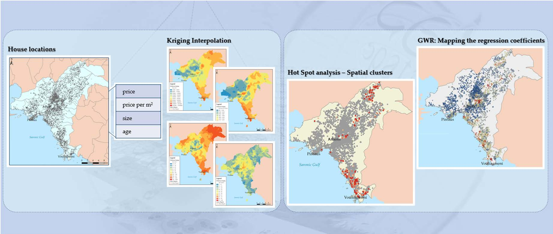
2. Materials and Methods

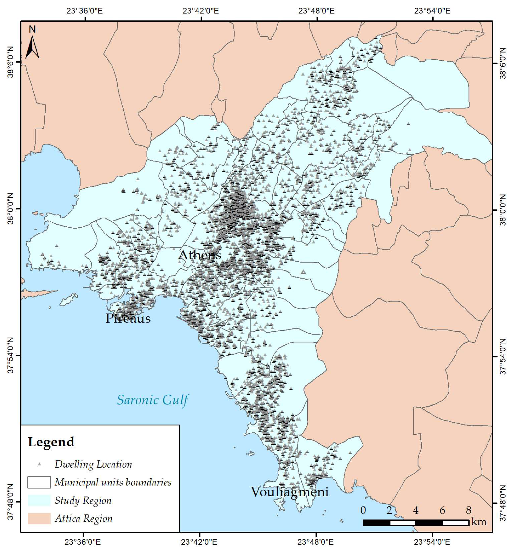
2.1. The Study Region and the Data

The study area is the Greater Athens region and consists of 57 municipal units, in which the greater number of houses for sale are concentrated. House data were obtained by entries concerning property for sale, published on the internet by real estate agencies (www.xe.gr, accessed on 28 March 2020). However, only houses for which the approximate location on a map was available were included in the sample. The location was recorded in Google maps and the resulting map was exported into a geodatabase. The sample comprises 4995 dwellings for sale in the first quarter of the year 2020 and the selection of the sample is proportionate to the number of houses in each municipal unit (Figure 1). Only residential property was included in the sample and all types of houses were recorded (apartments and single family houses). Several structural characteristics were derived from the real estate web pages, such as price, size, age, floor, number of bedrooms, bathrooms, parking, view and fireplace.
In addition, some locational characteristics were created in a GIS environment, as follows: distance from the center of the city, distance from the closest metro station and distance from the beach. The first two variables are common in the relevant literature [6,7,8,11,13,15], while distance from the beach is important for the study region since some of the most expensive areas are close to the sea. Locational attributes represent the desirability of each neighborhood; therefore, they can be considered as neighborhood characteristics as well [6,7]. Other neighborhood characteristics, such as crime, would be important for the analysis, especially for the center of Athens, however they are not available for the entire study region. Furthermore, socioeconomic characteristics were not incorporated in the analysis, although they are highly correlated to property values [1]. Socioeconomic data, such as educational attainment, sector of economic activity, occupational status and unemployment, are available for municipalities, which are quite large areas. If values to each house were attributed through GIS operations, they would be identical for all houses in the same municipality and they would not be very useful for statistical analysis.

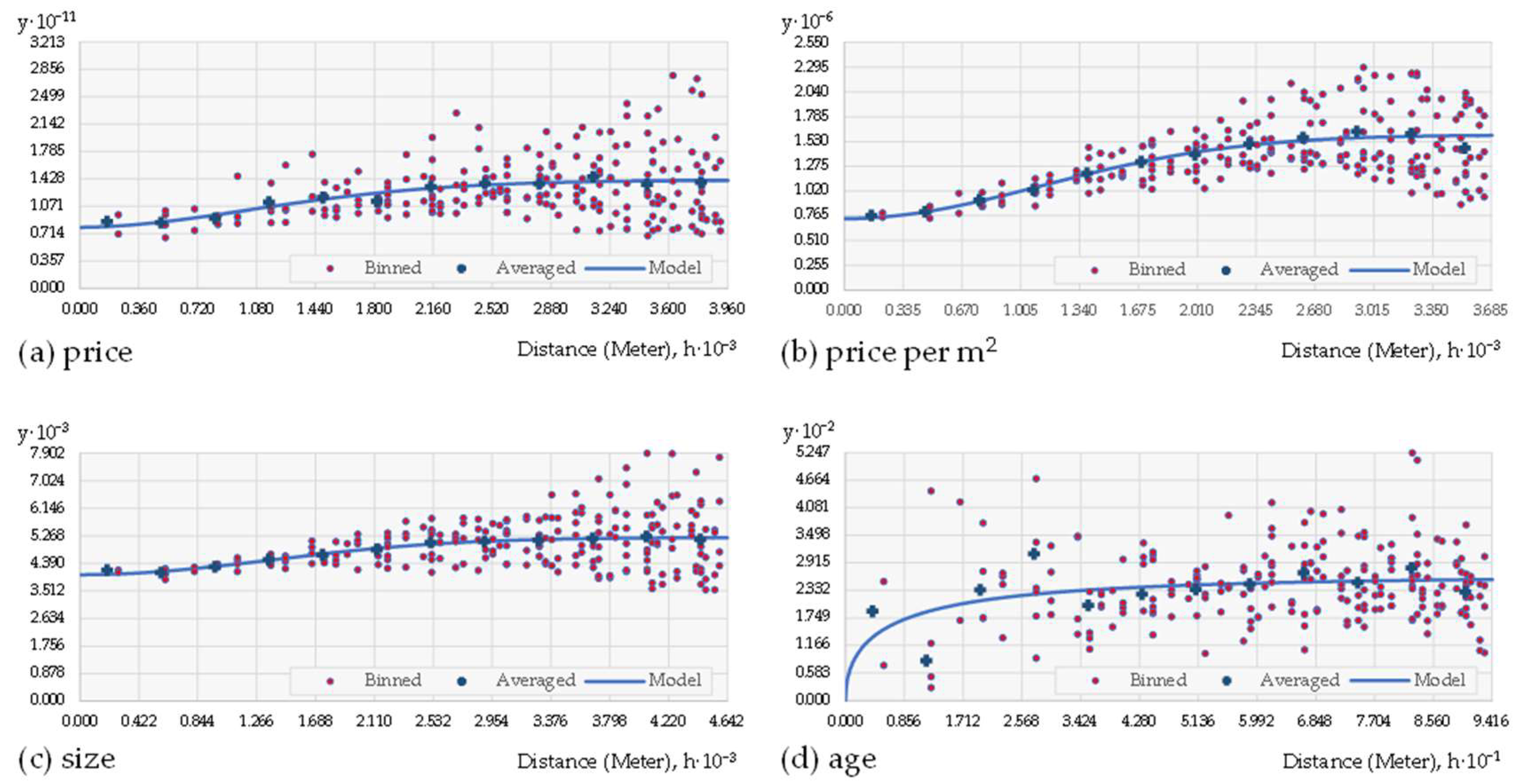
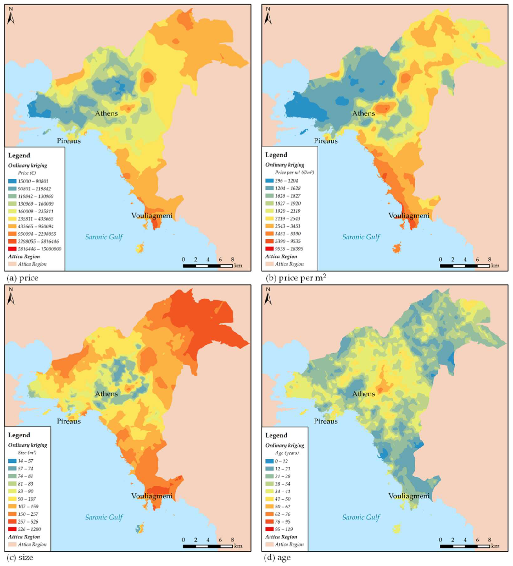
2.2. Geovisualization of the Data with Kriging Analysis

At first, a description of the houses in the sample is presented, in terms of their structural characteristics. Since we are dealing with point data, a kriging interpolation analysis [24] was considered appropriate for geovisualization and was carried out for selected variables.
Spatial interpolation is the prediction of values of attributes at unsampled locations from measurements made at sample points in the same area. Therefore, interpolation is a type of spatial prediction and results in a continuous surface. The principle underlying spatial interpolation is the first law of geography. Formulated by Waldo Tobler [25], this law states that everything is related to everything else, but near things are more related than distant things. This is also the classic definition of spatial autocorrelation.
There are several methods of interpolation that can be classified into two groups: deterministic and geostatistical. Deterministic techniques assume no measurement error and use mathematical functions for interpolation, while geostatistical methods rely on both statistical and mathematical methods, which, apart from creating surfaces, can assess the uncertainty of the predictions [5]. In spatial interpolation methods, the values of attributes at certain locations are calculated employing a set of weights. For example, inverse distance weighting (IDW) is a common deterministic method and the weights are calculated as a function of distance. To predict a value for any unmeasured location, IDW uses the measured values surrounding the prediction location. In principle, the measured values closest to the prediction location have more influence on the predicted value than those farther away. IDW assumes that each measured point has a local influence that diminishes with distance. It gives greater weights to points closest to the prediction location, and the weights diminish as a function of distance. On the other hand, geostatistical interpolation techniques, i.e., kriging, utilize the statistical properties of the measured points. Kriging is a statistical interpolation method which assumes that at least some of the spatial variation observed in the data can be modelled by random processes and requires that spatial autocorrelation is explicitly modelled. Kriging techniques can be used to describe and model spatial patterns, predict values at unmeasured locations and create prediction surfaces but, also, they calculate the error associated with them.
Kriging analysis has been used in several studies for the analysis of house prices [26,27]. Due to the uncertainty as to the location of the house data in this study, a kriging interpolation technique is used in order to describe the spatial patterns of house characteristics. Kriging involves quantifying the spatial structure of the data by creating the semivariogram, which is a plot of the squared differences in the values of the sample points against the distance between them. To make a prediction for an unknown value for a specific location, kriging will use a fitted model from variography, the spatial data configuration, and the values of the measured sample points around the prediction location. There are several different types of kriging, according to the assumptions about the properties of the field being interpolated [28,29]. In this study, ordinary kriging is employed, which is one of the most often used types of kriging.

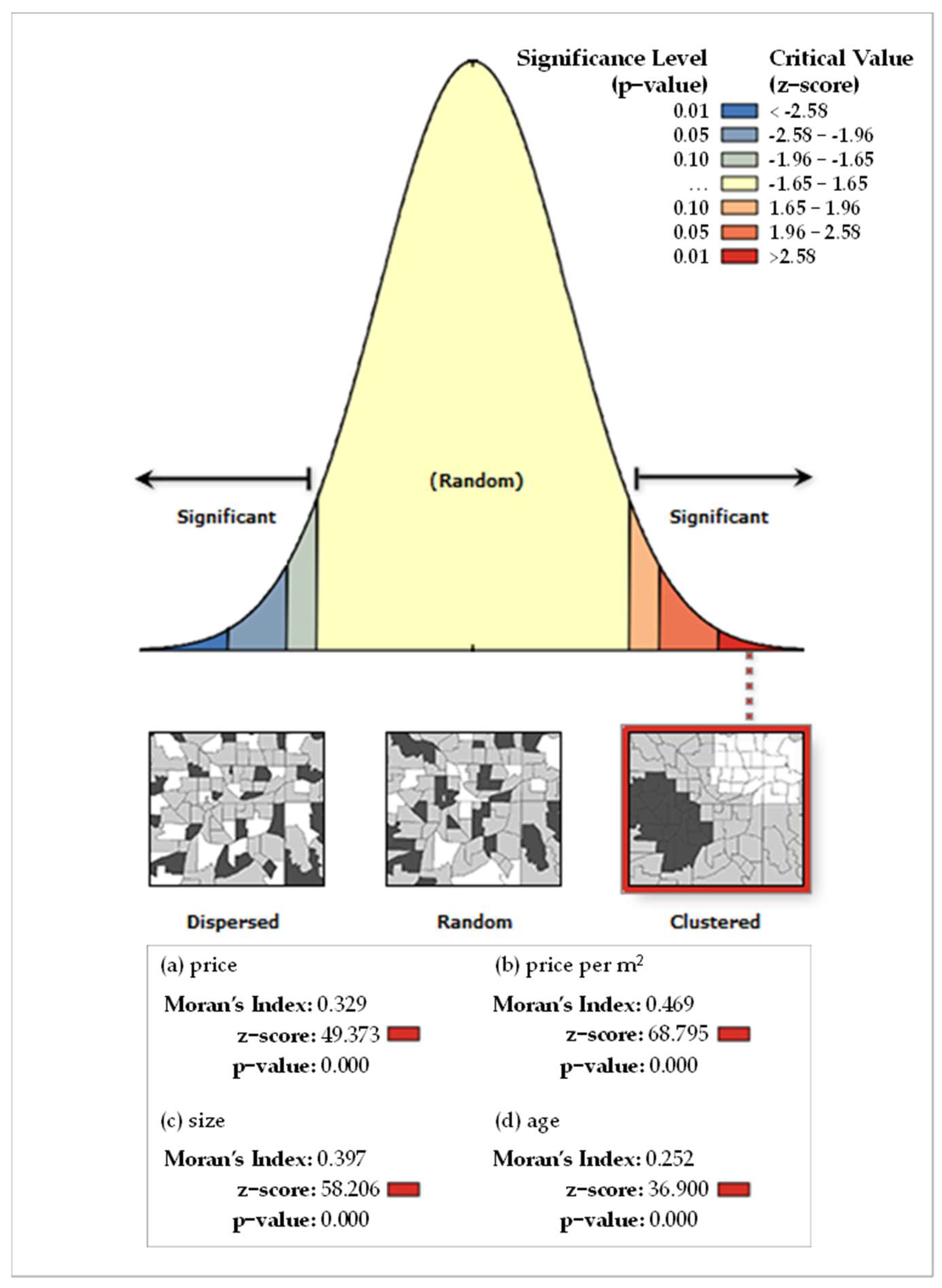
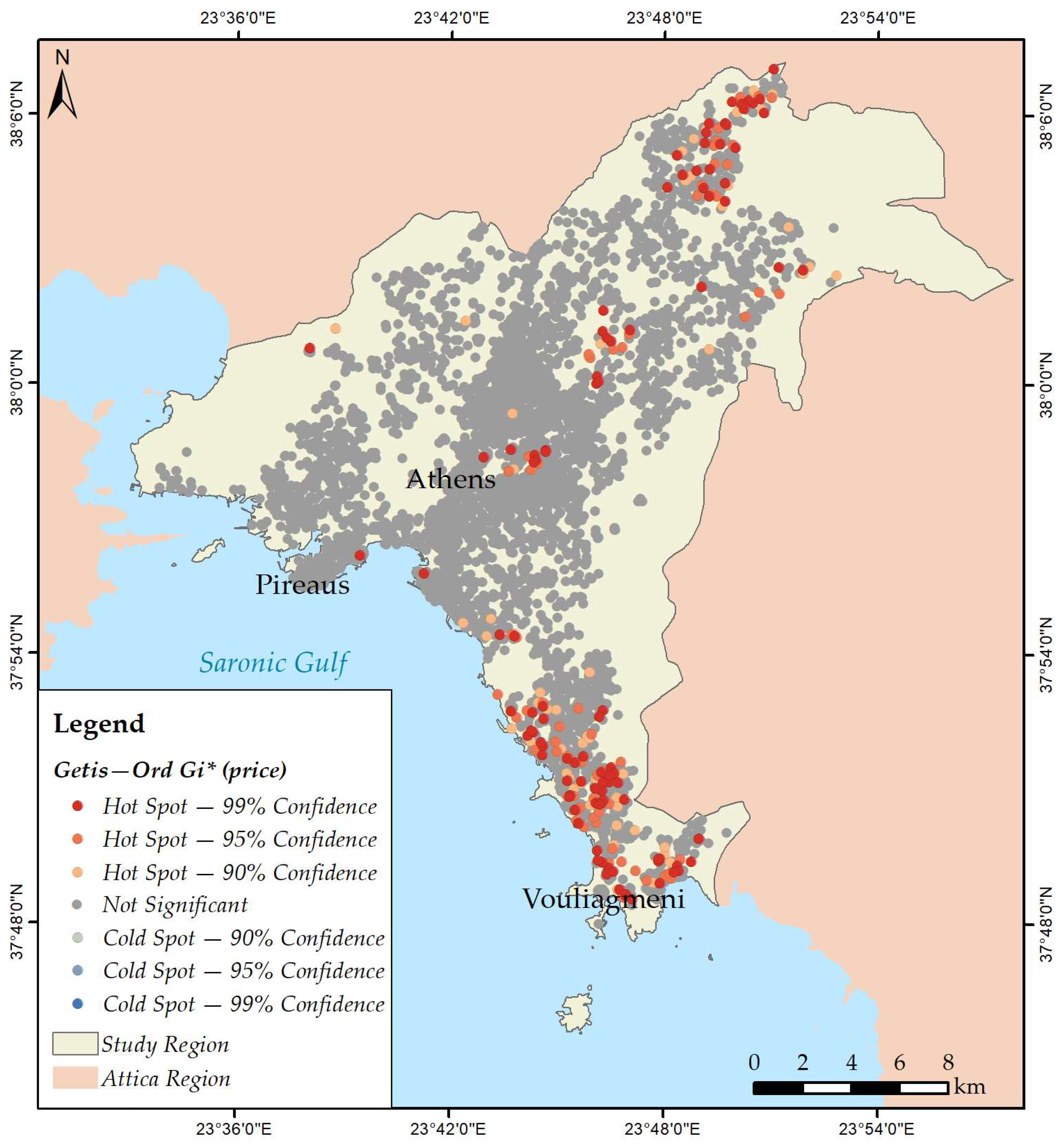
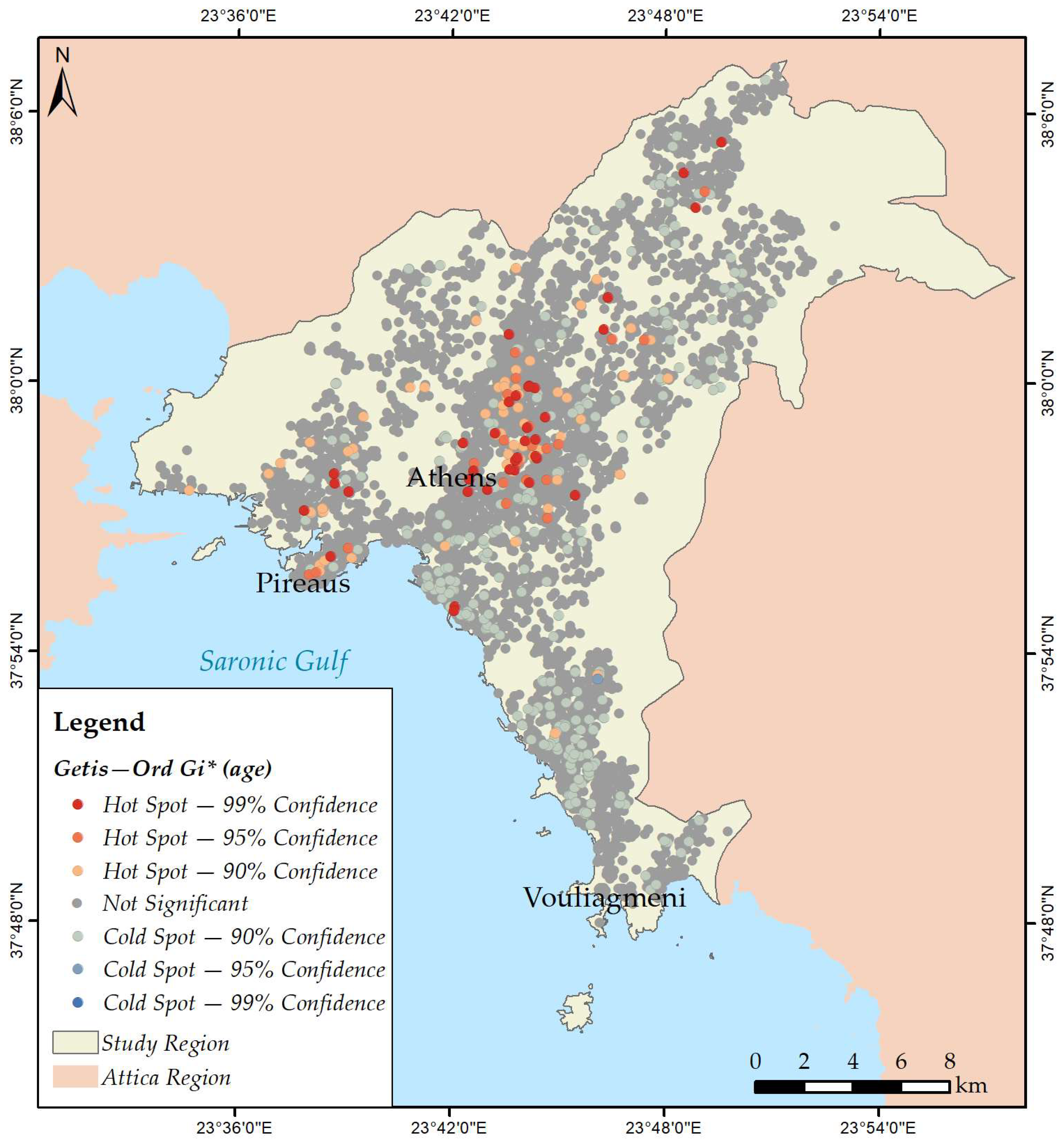
2.3. Mapping Spatial Clusters

The second procedure is the identification of spatial clusters through the measurement of spatial autocorrelation. There are several indices of spatial autocorrelation, such as the Moran’s I and the Geary’s C. In order to measure spatial autocorrelation, the spatial structure of the data has to be described and, for that purpose, a matrix of spatial weights is constructed. Locations at smaller distances are expected to share similar values for the attributes in question and this property is accounted for in the construction of spatial weights. There is a wide variety of methods to define spatial weights. For point data, some function of distance is used, such as the inverse distance. In this study, the inverse distance squared method is used. The most widely used measure of spatial autocorrelation is the Moran’s I coefficient, which employs a covariance term between each spatial unit and its neighbors. Spatial autocorrelation can be positive or negative, indicating clustering or dispersion. In that case, the values of the Moran’s index are positive and negative, respectively. Values are in the range of −1 to +1 and a value of zero indicates a random spatial pattern. The calculation of the values of Geary’s C coefficient are different, but the interpretation of the results is similar [5]. These coefficients are the global ones, measuring spatial autocorrelation for the whole dataset.
The statistical significance of the autocorrelation coefficients is tested through randomization tests or resampling [30]. The values of the observations are randomly rearranged in order to create different spatial arrangements, for 1000 or 10,000 times, and the spatial autocorrelation coefficient is calculated for each dataset. The result is an experimental distribution from which an inference about the observed distribution can be derived. If the coefficient based on the observed distribution is sufficiently distant from the mean of the experimental distribution, it is plausible to conclude that the spatial distribution of the observed data is highly unlikely to have arisen from a random process. Conversely, if the coefficient for the observed distribution is not sufficiently far from the mean of the experimental distribution, it is concluded that a random process is in operation.
On the other hand, local measures of spatial autocorrelation, such as the Local Moran’s I and the Getis–Ord Gi*, can indicate the location of clusters of observations with high or low values [5,21,22]. The local coefficient Moran’s I is derived in a similar way as the global statistic, but for smaller areas within the study region. The Getis–Ord Gi* statistic aims to detect local concentrations of high or low values in an attribute, so spatial clusters of low or high values can be identified in the dataset. It is also referred to as hot-spot analysis. The calculation of the Getis–Ord Gi* index involves the spatial weights and the values at different locations in the neighborhood of the location of interest. In a location where high values are clustered, Gi* will be relatively high; conversely, in a location where low values are concentrated, Gi* will be low.
In this study, the global Moran’s I is used as a means to test global spatial autocorrelation for selected variables and, if a positive spatial autocorrelation is detected, the Getis–Ord Gi* index is used to map the clusters of high or low values for selected variables. The resulting spatial patterns are compared with the kriging interpolation maps.

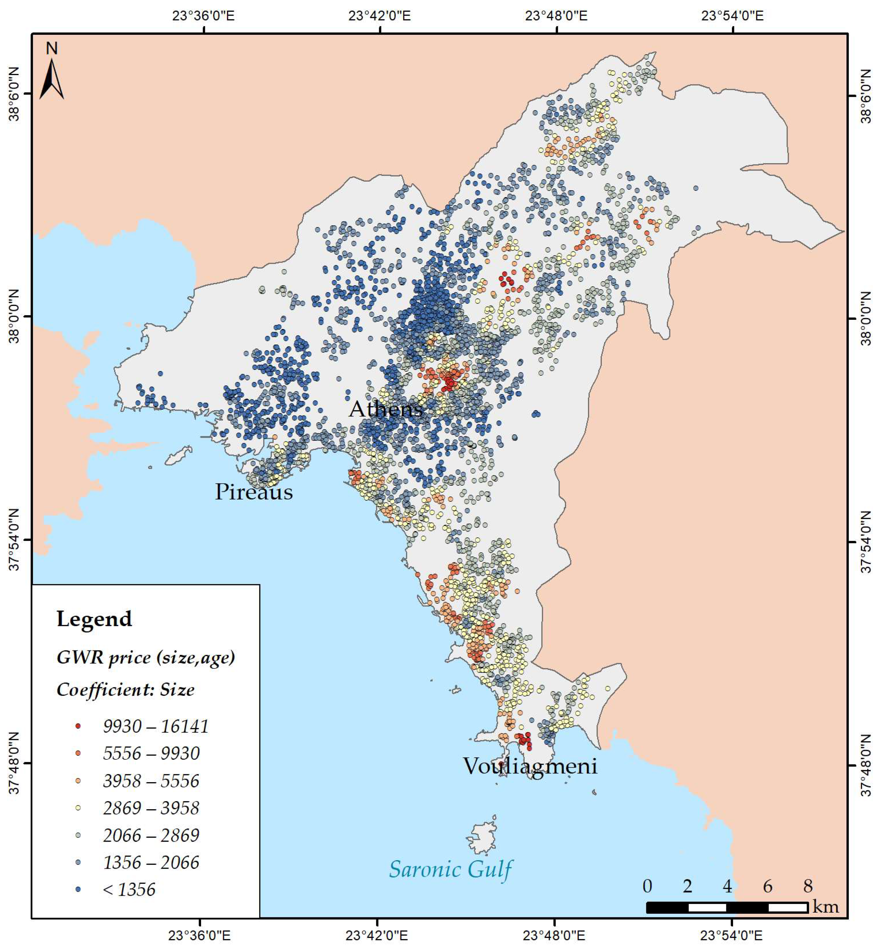
2.4. Regression Models

The final step of the analysis is the construction of a regression model in order to predict house prices from a series of house characteristics. Regression analysis involves one independent variable and one or more independent variables, the covariates or explanatory factors. The purpose of regression analysis is to create a model in order to predict values of the dependent variable for observations where there is no measurement. For hedonic pricing models, regression analysis is extremely important, because it makes it possible to estimate house prices given that the house characteristics are known. Regression analysis includes a great variety of models, but the model to begin with is linear regression. In linear regression, the dependent variable is a linear function of the independent variables. Simple linear regression involves only one independent variable, while multiple regression two or more independent variables. The equation for multiple linear regression is as follows:
Y = a + b 1 X 1 + b 2 X 2 + + b n X n + e
where Y is the dependent variable, Xi are the independent variables, a is a constant, bi are the regression coefficients and e is the error term. The quantities a and bi are the parameters that define the model and are estimated from the data. The regression coefficients measure the impact of each independent variable on the dependent variable. However, if the regression coefficients are going to be compared in terms of their impact, then the independent variables have to be standardized. In that case, the regression coefficients are transformed to beta coefficients. This model is global, in the sense that the regression equation is the same for all the study region and all the data have been used for its estimation. The error term (or residuals), however, is different for each observation and is the difference between the observed and the estimated value of the dependent variable for each observation. Linear regression uses the minimization of the sum of the squared residuals as the condition for the calculation of the regression parameters, hence the term ordinary least squares (OLS) model [31]. For geographical datasets, residuals can be mapped and reveal spatial patterns.
Many assumptions are associated with linear regression, the most important one being the linear relationship between the dependent and the independent variables. This hypothesis can be tested through bivariate scatter diagrams and correlation analysis, i.e., the calculation of the Pearson correlation coefficient. The most important measure to evaluate the goodness of fit of the model is the coefficient of determination, which is the proportion of the variance of the dependent variable explained by the independent variables. This is reported as R square (R2) and is the squared Pearson correlation coefficient, with values ranging between 0 and 1. Therefore, if there is a strong linear relationship between the dependent and the independent variables, the coefficient of determination will be close to 1, indicating an accurate prediction of the dependent variable. Through correlation analysis, the relationship among the independent variables can be tested and multicollinearity can be identified, when two or more independent variables are related to each other. Another important assumption for regression analysis is the independence of the residuals. This assumption is very often violated for geographical problems, since data are spatially autocorrelated. Therefore, the regression model is misspecified and, in order to remedy this situation, spatial regression models have been developed that analyze spatial data. The spatial dependency of the residuals is tested through a measure of spatial autocorrelation, such as the Moran’s I.
There is a variety of spatial regression models, which all engage spatial autocorrelation in the calculations of the parameters. In order to account for spatial autocorrelation in the data, there are two basic approaches [31]. The first approach is to include an independent variable, which is created by the values of the dependent variable for all the neighboring observations of each target location. This is a spatially lagged variable and is a weighted sum or a weighted average of the neighboring values for that variable [21]. The second approach is to create a model that allows spatial variation of the regression parameters and this is the geographically weighted regression (GWR) model [22]. The basic principle in this approach is that a global model is not representative for all the locations in the study area. GWR is a local regression model, since it constructs a separate regression equation for every location in the dataset. The equation incorporates the dependent variable and the explanatory variables of locations falling within the bandwidth of each target location. The regression coefficients vary across the study region and it is possible to evaluate the importance of each independent variable in different parts of the study region.
In this study, an OLS model is initially estimated incorporating quantitative variables as well as some binary variables. In the case of a large number of independent variables, there are methods for selecting the variables so that multicollinearity is avoided [32]. The stepwise elimination method is used in this analysis. The OLS residuals are tested for randomness using the Moran autocorrelation coefficient and, if they are clustered, a GWR regression model is estimated.

3. Results

The dataset includes several variables concerning the following house characteristics:
  • Price;
  • Price per m2;
  • Size;
  • Age;
  • Floor number;
  • Number of rooms;
  • Number of bathrooms;
  • Existence of parking;
  • Existence of view;
  • Existence of fireplace;
  • Distance from the center;
  • Distance from the nearest metro station;
  • Distance from the beach.
Variables 1–7 and 11–13 are quantitative, while the rest (i.e., parking, view and fireplace) indicate the presence or absence of certain amenities. In addition, variables 5–7 represent quantitative characteristics but they have a small number of discrete values. Only continuous quantitative variables describing prices, and two structural characteristics (size and age) were examined in terms of spatial clustering. This selection is based on the importance of these characteristics and, also, the data properties, which affect the results of kriging and hot-spot analyses. In the regression models, all variables were introduced, with the exception of three variables, i.e., “price per m2”, “number of rooms” and “number of bathrooms”, due to redundant information in these independent variables (see Section 3.3). Data analysis was carried out employing ArcGIS v.10.8 for geostatistical, hot-spot and GWR analysis, while IBM SPSS v.27 was used for OLS analysis.

3.1. Kriging Analysis and Measures of Spatial Autocorrelation

Ordinary kriging results for the variables “price”, “price per m2”, “size” and “age” are shown in Figure 2 and Figure 3 and Table 1. The results for each variable comprise the interpolation map, the empirical semivariogram and the diagnostics for the fit of the model. The classification applied in the interpolation map was carried out by using the optimization method of classes’ distribution natural breaks. The Jenks optimization method, also called the “Jenks natural breaks classification method”, is a data classification method designed to determine the best arrangement of values into different classes. This is performed by seeking to minimize each class’s average deviation from the class mean, while maximizing each class’s deviation from the means of the other groups. In other words, the method seeks to reduce the variance within classes and maximize the variance between classes [33].
Each dot in the semivariogram (Figure 3) represents a group of locations at small distances. This is the binning process, which is applied for large datasets. If data are spatially dependent, the points that are close together should have smaller differences. As points become farther away from each other, in general, the difference squared should be greater. There is a certain distance beyond which the squared difference levels out and the locations beyond this distance are considered to be uncorrelated. In addition, a fitted model is presented, which is used to create the prediction surface. Two are the most important diagnostics for kriging analysis: the mean standardized (MS), which has to be close to zero, and the root mean square standardized (RMSS), which has to be close to 1. The results indicate a very good fit for all variables, with the exception of the variables “price” and “size”, for which RMSS > 1.
For the better interpretation of the kriging analysis, the global Moran’s I index of spatial autocorrelation for the selected variables was calculated and the results are shown in Figure 4. The values of the Moran’s index are in the range of −1 to +1, with an index score greater than 0.3 being an indication of relatively strong autocorrelation. The empirical distributions of Figure 4 are interpreted as in classic inference with normal distribution, calculating the z-values of the coefficient and the associated p-value. The results for all variables indicate a clustered spatial pattern at a 0.01 significance level.

3.2. Mapping Spatial Clusters

The Getis–Ord Gi* coefficient was calculated for the variables “price”, “price per m2”, “size” and “age” in order to identify hot spots and cold spots, i.e., clusters of houses with high or low values for these characteristics. For the conceptualization of spatial relationships, the inverse distance squared option was selected, which results in decreasing the influence of neighboring observations with distance. The results of this procedure are presented in Figure 5, Figure 6, Figure 7 and Figure 8, in which the significance of the Gi* statistic is mapped.

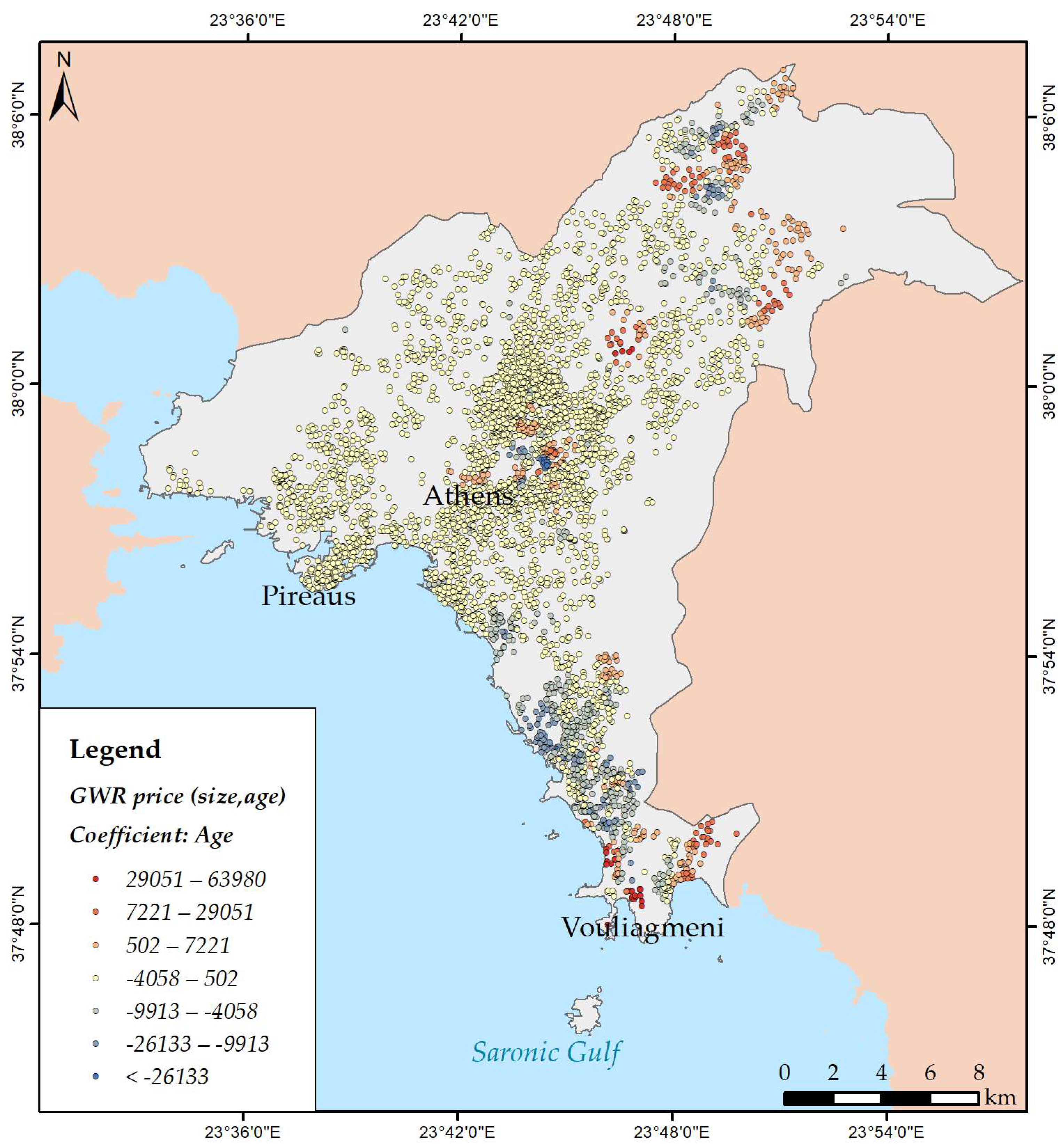
3.3. Modelling Spatial Relationships

The final part of the analysis concerns a regression model that will explain the spatial variation in house prices and predict house prices for locations outside the sample data. As spatial data are analyzed, the aim is a spatial regression (GWR) model. The starting point, however, is a linear regression model (OLS) and if spatial autocorrelation causes misspecification problems, a spatial regression model would be more appropriate [21]. The OLS model can be calculated with conventional statistical analysis software but also in a GIS environment. However, when using statistical analysis software for the OLS model, it is easier to address multicollinearity problems and select independent variables that are not correlated with each other. In this way, only data without multicollinearity will enter the GWR model. For the OLS model, the dependent variable is house price (“price”) and all variables listed in Section 3 were included as independent variables, with the exception of “price per m2”, “number of rooms” and “number of bathrooms”. “Price per m2” is derived from the variables “price” and “size” and it could be a dependent variable, while the number of rooms and bathrooms represent similar information as size. Three binary variables were entered as well: “parking”, “fireplace” and “view”. Therefore, nine independent variables were included in the analysis.
The initial linear regression model with all variables indicated several not significant regression coefficients. For that reason, a stepwise procedure was applied, which produced a model with five independent variables (Table 2). In Table 2, the regression coefficients and their significance are presented, together with the beta coefficients. The goodness of fit of the model is determined by the adjusted R2, which has a value of 0.583, indicating a moderate fit.
In order to improve the fitting of the model, several procedures can be followed. A common procedure is to transform the dependent and/or the independent variables, usually employing a logarithmic transformation [34]. Other studies apply spatial regression models which are calculated in a GIS environment and they take into consideration the location of the observations and the property of spatial autocorrelation [1,35].
Subsequently, the residuals of the OLS procedure were tested for spatial autocorrelation. The Moran’s I indicated that the residuals are clustered at the 0.01 significance level. Therefore, an improvement in the model can be expected when taking into consideration the spatial autocorrelation in the data. Initially, all five independent variables of the OLS procedure were introduced into a GWR model, but this yielded no results, due to spatial multicollinearity issues [36,37]. Accordingly, different combinations of variables were tested for building a GWR model starting with “size” and gradually adding variables, so that R2 would be maximized (Table 3). The variable with the highest adjusted R2 in bivariate regression is “size” and then “age”, “view”, “parking” and “distance from the beach”. The adjusted R2 for different GWR models is presented in Table 3. In the end, the best fit is for the model with “price” as the dependent variable and “size” and “age” as the independent variables. This model has a high explanatory power with an adjusted R2 of 84.8%. The variable “distance from the beach” was not, finally, included because of local multicollinearity problems and the binary variables did not increase the explanatory power of the model, when more than one variable was introduced. However, it has to be noted that the contribution of “age” in the explanatory power of the model is quite small (3.6%).
The results of this model indicated a much higher explanatory power in comparison to OLS (Table 4). In addition, the Akaike information criterion (AIC) decreased, indicating a better fir of the GWR regression model [38].
The GWR model calculates a regression equation for each observation, a house in this study. As observed, there is a spatial variation of the coefficients, which can be interpreted as the spatial variation of the impact of each factor for the determination of house prices. In Figure 9 and Figure 10 the spatial variation of the coefficients for the independent variables “size” and “age” are presented, respectively.

4. Discussion

The results of the kriging analysis in Section 3.1 present the spatial patterns for four house characteristics: price, price per m2, size and age. For all these variables, the semivariograms model spatial autocorrelation, while the Moran’s I index (Figure 4) suggests quite strong spatial autocorrelation and a clustered spatial pattern. In addition, the diagnostics for ordinary kriging indicate a good fit of the model.
Figure 2a shows the spatial distribution of house prices in the study region. There is a pattern which has been reported in other studies for the Athens region [1,3] indicating low prices at the western parts of the city and higher prices at the northern and southern suburbs. In addition, expensive houses are found at the center of the city and in some municipal units (Filothei and Psychiko) close to the center. Figure 2b presents the price per m2 and the resulting spatial pattern is similar to the previous one for “price”; however, the distinction between the western suburbs, on the one hand, and the southern and northern suburbs, on the other, is more obvious. The spatial pattern for the variable “size” suggests that smaller houses are mostly concentrated in some neighborhoods of Athens. The municipality of Athens includes several neighborhoods with quite different characteristics, which mostly reflect socioeconomic differences and not differences in building regulations or the age of the buildings. Therefore, apartment buildings are the prevailing type of housing, however, the quality of buildings and the structural characteristics, such as size, are different, resulting in differences in house prices as well. On the other hand, large houses are found in several areas, but the larger houses are in the northern and southern suburbs, where the house prices are also high (see Figure 2a–c). Therefore, price and size of the houses seem to be spatially correlated. Finally, the spatial pattern for the age of the houses indicates that the older houses are found in the municipality of Athens and this is reasonable since the center is the oldest part of the study region, with the urban expansion towards the suburbs being implemented in subsequent time periods.
In terms of mapping spatial clusters, the Getis–Ord Gi* produced maps of hot spots, and no cold spots, with the exception of the variable “age,” for which cold spots of lower significance (90%) are detected. For the variable “price” (Figure 5), two main clusters of high prices (hot spots) are identified, at the northern and southern suburbs of Athens. In addition, high prices are found at the center of Athens and in two municipal units close to the center (Psychiko and Filothei). For the variables “price per m2” and “size”, similar clusters of high prices (hot spots) are observed as for “price”. The spatial clusters for “age” indicate hot spots of old buildings at the center of Athens and Piraeus and cold spots mostly at the southern suburbs of Athens.
Therefore, two geovisualization methods, i.e., kriging analysis and hot-spot analysis produced similar results, indicating a quite clear spatial differentiation in the study region. The northern and southern suburbs are characterized by high house prices and larger properties, relatively new in age. In addition, some parts of the center of the city have high prices, although in general the houses are older and of smaller size. Finally, two municipal units, Psychiko and Filothei, are characterized by high prices and large properties. These findings are related to the socioeconomic characteristics in the study region [1]. In the center of the city, some of the most expensive areas in the study region are traditionally located in close proximity to the parliament and the central square of the city, named Syntagma Square. The northern suburbs are characterized by large properties and extended private or public green areas, which, for several decades, have been the residence of entrepreneurs and, in general, of higher status population groups. The southern suburbs are characterized by more recent growth and house prices are high due to the proximity to the sea and the construction of the new airport in the early 2000s. Psychiko and the neighboring Filothei have been built according to town plans characterized by a circular road pattern and the presence of green areas. Several embassies are located in Psychiko and the socioeconomic status of the residents is related to high house prices. The rest of the study region is in general characterized by lower prices, while the differences in size and age are not important.
In terms of creating a hedonic model for estimating house prices, two models were presented: the ordinary least squares model and the geographically weighted regression (GWR) model. For the OLS model, the dependent variable was “price” and the independent variables were five structural characteristics (size, age, floor, parking and fireplace) and four locational attributes, including view and distances from the city center, the metro stations and the beach. However, due to multicollinearity issues, five independent variables remained in the model: “size”, “age”, “distance from the beach”, “parking” and “view”. The results of the OLS regression model, especially the standardized beta coefficients, indicate that size is the most important factor for estimating house prices. This result is consistent with the findings of other studies [1,39,40]. Only one of the variables describing distances from points of interest was included in the OLS model (distance from the beach). Locational attributes although extremely important for house prices do not have a linear relationship with prices, especially for a large area such as the study region. After some critical distance, for example a walking distance or a short drive, it does not matter if the distance increases. In that case, statistical testing can show the effect on house prices [3].
The goodness of fit for this model is rather moderate, as indicated by an adjusted R2 with a value of 0.583. In addition, the OLS residuals proved to be spatially clustered, suggesting misspecification of the regression parameters. Therefore, a spatial regression model (GWR) was investigated in order to improve the results. After several trials, the proposed GWR model has “price” as the dependent variable and “size” and “age” as the independent variables, however the results indicate that the variable “size” accounts for most of the variability in “price”. The locational attributes were not useful in the GWR context, because of local multicollinearity issues. The explanatory power of the model is significantly higher relative to the OLS model, with an adjusted R2 of 0.848. It is remarkable that the increased explanatory power is obtained with only two independent variables, instead of five in OLS. This is very useful for estimating house prices, since fewer house characteristics are needed for a mass appraisal model. In several studies, spatial regression models are used for the creation of the hedonic models [1,3,4,17,20,23], since they can capture the spatial autocorrelation properties of spatial data.
A very important advantage of GWR is that it creates local regression models and allows for the spatial variation of regression coefficients. The results produce regression coefficient surfaces and can lead to conclusions as to the importance of an explanatory factor in different parts of the study region. In Figure 9, the GWR regression coefficient for “size” is mapped, resulting to a quite clear spatial pattern. The smaller regression coefficients for size are observed mostly in the western parts of the study region, but also in several neighborhoods of Athens, where lower prices are prevailing (see Figure 2). On the contrary, larger regression coefficients are observed in the areas with high prices, especially Vouliagmeni, which is the most expensive region in Attica. In these areas, large sizes are accompanied by other amenities, such as the existence of a swimming pool. In Figure 10, the GWR regression coefficient for “age” is mapped. In most parts of the study region, negative coefficients for age are observed, as expected. The largest negative coefficients are observed in an expensive neighborhood at the center of Athens (Rigillis). On the other hand, positive coefficients for “age” are found in the expensive areas of the city, which were previously identified, although negative coefficients are observed there as well. For the interpretation of positive age coefficients specific knowledge for these houses is required, if, for example, they are houses of certain historical or architectural value.
In this study, the spatial patterns for house characteristics were presented using statistical techniques: kriging and hot-spot analyses. This type of visualization engages all points in the dataset and produces detailed spatial patterns, while the statistical significance of the results is presented. The regression models showed that working with spatial data, and especially a GWR model, can significantly increase the explanatory power of an OLS model. Since house data are inherently spatial, it seems that if hedonic models incorporate spatial regression techniques, they can improve the accuracy of prediction employing fewer house characteristics as independent variables.

Author Contributions

Conceptualization, P.I.; methodology, P.I.; formal analysis, P.I. and E.F.; investigation, P.I.; writing—original draft preparation, P.I.; writing—review and editing, P.I. and E.F.; supervision, P.I.; visualization, E.F. All authors have read and agreed to the published version of the manuscript.

Funding

This research received no external funding.

Data Availability Statement

The data presented in this study are available on request from the corresponding author. The data are not publicly available due to copyright restrictions. The open data used in this study are provided in the website: http://geodata.gov.gr/dataset (accessed on 11 November 2021).

Acknowledgments

The authors would like to thank the Geospatial Technology Research Lab (GAEA) of the University of West Attica for the provision of the house data.

Conflicts of Interest

The authors declare no conflict of interest.

References

  1. Iliopoulou, P.; Stratakis, P. The geography of housing prices in the Greater Athens Region, Greece: Patterns, Correlations and trends. In Innovative Geographies: Understanding and Connecting Our World, Proceedings of the 11th International Conference of the Hellenic Geographical Society, Lavrion, Greece, 12–15 April, 2018; Govostis Publisher Co.: Athens, Greece, 2018; Available online: http://www.geochoros.survey.ntua.gr/hgs/el/11th-conference-proceedings?field_topic_tid=All&title=&title_field_value_1=iliopoulou (accessed on 8 December 2021).
  2. Stamou, M.; Mimis, A.; Rovolis, A. House Price Determinants in Athens: A Spatial Econometric Approach. J. Prop. Res. 2017, 34, 269–284. [Google Scholar] [CrossRef]
  3. Iliopoulou, P.; Stratakis, P. Spatial Analysis of Housing Prices in the Athens Region, Greece. RELAND Int. J. Real Estate Land Plan. 2018, 1, 304–313. [Google Scholar]
  4. Fotheringham, A.S.; Crespo, R.; Yao, J. Exploring, Modelling and Predicting Spatiotemporal Variations in House Prices. Ann. Reg. Sci. 2015, 54, 417–436. [Google Scholar] [CrossRef]
  5. O’Sullivan, D.; Unwin, D. Geographic Information Analysis; John Wiley & Sons: Hoboken, NJ, USA, 2003; ISBN 978-0-471-21176-1. [Google Scholar]
  6. Baranzini, A.; Ramirez, J.; Schaerer, C.; Thalmann, P. Hedonic Methods in Housing Markets: Pricing Environmental Amenities and Segregation; Springer Science & Business Media: New York, NY, USA, 2008; ISBN 978-0-387-76815-1. [Google Scholar]
  7. Bhattacharjee, A.; Castro, E.; Marques, J. Spatial Interactions in Hedonic Pricing Models: The Urban Housing Market of Aveiro, Portugal. Spat. Econ. Anal. 2012, 7, 133–167. [Google Scholar] [CrossRef]
  8. Xiao, Y. Urban Morphology and Housing Market; Springer Geography: Singapore, 2017; ISBN 978-981-10-2761-1. [Google Scholar]
  9. Anderson, S.T.; West, S.E. Open Space, Residential Property Values, and Spatial Context. Reg. Sci. Urban Econ. 2006, 36, 773–789. [Google Scholar] [CrossRef] [Green Version]
  10. Cho, S.-H.; Poudyal, N.C.; Roberts, R.K. Spatial Analysis of the Amenity Value of Green Open Space. Ecol. Econ. 2008, 66, 403–416. [Google Scholar] [CrossRef]
  11. Efthymiou, D.; Antoniou, C. How Do Transport Infrastructure and Policies Affect House Prices and Rents? Evidence from Athens, Greece. Transp. Res. Part A Policy Pract. 2013, 52, 1–22. [Google Scholar] [CrossRef]
  12. Luttik, J. The Value of Trees, Water and Open Space as Reflected by House Prices in the Netherlands. Landsc. Urban Plan. 2000, 48, 161–167. [Google Scholar] [CrossRef]
  13. McMillen, D.P.; McDonald, J. Reaction of House Prices to a New Rapid Transit Line: Chicago’s Midway Line, 1983–1999. Real Estate Econ. 2004, 32, 463–486. [Google Scholar] [CrossRef]
  14. Sander, H.A.; Polasky, S. The Value of Views and Open Space: Estimates from a Hedonic Pricing Model for Ramsey County, Minnesota, USA. Land Use Policy 2009, 26, 837–845. [Google Scholar] [CrossRef]
  15. Raslanas, S.; Tupenaite, L.; Šteinbergas, T. Research on the Prices of Flats in the South East London and Vilnius. Int. J. Strateg. Prop. Manag. 2006, 10, 51–63. [Google Scholar] [CrossRef]
  16. Pek, J.; Wong, O.; Wong, A. Data Transformations for Inference with Linear Regression: Clarifications and Recommendations. Pract. Assess. Res. Eval. 2019, 22, 9. [Google Scholar] [CrossRef]
  17. De Bruyne, K.; Van Hove, J. Explaining the Spatial Variation in Housing Prices: An Economic Geography Approach. Appl. Econ. 2013, 45, 1673–1689. [Google Scholar] [CrossRef]
  18. Lake, I.R.; Lovett, A.A.; Bateman, I.J.; Day, B. Using GIS and Large-Scale Digital Data to Implement Hedonic Pricing Studies. Int. J. Geogr. Inf. Sci. 2000, 14, 521–541. [Google Scholar] [CrossRef]
  19. Mimis, A.; Rovolis, A.; Stamou, M. Property Valuation with Artificial Neural Network: The Case of Athens. J. Prop. Res. 2013, 30, 128–143. [Google Scholar] [CrossRef]
  20. Pace, R.K.; Barry, R.; Sirmans, C.F. Spatial Statistics and Real Estate. J. Real Estate Financ. Econ. 1998, 17, 5–13. [Google Scholar] [CrossRef]
  21. Anselin, L.; Rey, S.J. Modern Spatial Econometrics in Practice: A Guide to GeoDa, GeoDaSpace and PySAL; GeoDa Press LLC: Chicago, IL, USA, 2014. [Google Scholar]
  22. Fotheringham, A.S.; Brunsdon, C.; Charlton, M. Geographically Weighted Regression: The Analysis of Spatially Varying Relationships Wiley Wiltshire; John Wiley & Sons: New York, NY, USA, 2002. [Google Scholar]
  23. Herath, S.; Choumert, J.; Maier, G. The Value of the Greenbelt in Vienna: A Spatial Hedonic Analysis. Ann. Reg. Sci. 2015, 54, 349–374. [Google Scholar] [CrossRef] [Green Version]
  24. Iliopoulou, P.; Kitsos, C. Kriging Analysis for Atmosphere Pollutants and House Prices: The case of Athens. In Economics of Natural Resources & the Environment, Proceedings of the 6th ENVECON Conference, Volos, Greece, 11–12 June 2021; Springer Science & Business Media: New York, NY, USA, 2012; pp. 233–247. Available online: http://envecon.econ.uth.gr/main/eng/images/6th_conference/6th_Conference_Proceedings.pdf (accessed on 12 December 2021).
  25. Tobler, W.R. A Computer Movie Simulating Urban Growth in the Detroit Region. Econ. Geogr. 1970, 46, 234–240. [Google Scholar] [CrossRef]
  26. Kuntz, M.; Helbich, M. Geostatistical Mapping of Real Estate Prices: An Empirical Comparison of Kriging and Cokriging. Int. J. Geogr. Inf. Sci. 2014, 28, 1904–1921. [Google Scholar] [CrossRef]
  27. Chica-Olmo, J.; Cano-Guervos, R.; Chica-Rivas, M. Estimation of Housing Price Variations Using Spatio-Temporal Data. Sustainability 2019, 11, 1551. [Google Scholar] [CrossRef] [Green Version]
  28. Cressie, N.A. Statistics for Spatial Data; John Willey & Sons, Inc.: New York, NY, USA, 1993. [Google Scholar]
  29. Isaaks, E.H.; Srivastava, R.M. Applied Geostatistics; Oxford Univ. Press: New York, NY, USA, 1989. [Google Scholar]
  30. Fotheringham, A.S.; Brunsdon, C. Some Thoughts on Inference in the Analysis of Spatial Data. Int. J. Geogr. Inf. Sci. 2004, 18, 447–457. [Google Scholar] [CrossRef]
  31. Rogerson, P.A. Statistical Methods for Geography: A Student’s Guide; SAGE: Southern Oaks, CA, USA, 2019; ISBN 978-1-5297-0023-7. [Google Scholar]
  32. Draper, N.R.; Smith, H. Applied Regression Analysis; John Wiley & Sons: New York, NY, USA, 1998; ISBN 978-0-471-17082-2. [Google Scholar]
  33. Jenks, G.F. The Data Model Concept in Statistical Mapping. Int. Yearb. Cartogr. 1967, 7, 186–190. [Google Scholar]
  34. Osborne, J. Improving Your Data Transformations: Applying the Box-Cox Transformation. Pract. Assess. Res. Eval. 2019, 15, 12. [Google Scholar] [CrossRef]
  35. Mankad, M.D. Analysis of Impact of Accessibility on Residential Property Values in Gotri Area of Vadodara City, India Using OLS and GWR. Int. J. Sci. Res. Sci. Eng. Technol. 2018, 4, 1118–1127. [Google Scholar] [CrossRef]
  36. Wheeler, D.C. Diagnostic Tools and a Remedial Method for Collinearity in Geographically Weighted Regression. Environ. Plan. A 2007, 39, 2464–2481. [Google Scholar] [CrossRef]
  37. Brunsdon, C.; Charlton, M.; Harris, P. Living with Collinearity in Local Regression Models. In Proceedings of the 10th International Symposium on Spatial Accuracy Assessment in Natural Resources and Environmental Sciences, Florianópolis, Brazil, 10–13 July 2012. [Google Scholar]
  38. Portet, S. A Primer on Model Selection Using the Akaike Information Criterion. Infect. Dis. Model. 2020, 5, 111–128. [Google Scholar] [CrossRef]
  39. Rodriguez, M.; Sirmans, C.F. Quantifying the value of a view in single family housing markets. Apprais. J. 1994, 62, 600–603. [Google Scholar]
  40. Ozgur, C.; Hughes, Z.; Rogers, G.; Parveen, S. Multiple Linear Regression Applications in Real Estate Pricing. Int. J. Math. Stat. Invent. 2016, 4, 39–50. [Google Scholar]
Figure 1. The study region and the sample of houses for sale.
Geographies 02 00008 g001
Figure 2. Ordinary kriging prediction maps for all four variables.
Geographies 02 00008 g002
Figure 3. Semivariograms for all four variables.
Geographies 02 00008 g003
Figure 4. Moran’s I for all four variables.
Geographies 02 00008 g004
Figure 5. Getis–Ord Gi*: “price”.
Geographies 02 00008 g005
Figure 6. Getis–Ord Gi*: price per m2.
Geographies 02 00008 g006
Figure 7. Getis–Ord Gi*: “size”.
Geographies 02 00008 g007
Figure 8. Getis–Ord Gi*: “age”.
Geographies 02 00008 g008
Figure 9. Geographically weighted regression (GWR): spatial variation in the size coefficient.
Geographies 02 00008 g009
Figure 10. Geographically weighted regression (GWR): spatial variation in the age coefficient.
Geographies 02 00008 g010
Table 1. Ordinary kriging diagnostics (prediction errors).
PricePrice Per m2SizeAge
Mean418.341.75−0.02−0.04
Root Mean Square393,947.31974.0781.1617.03
Mean Standardized0.0010.002−0.000−0.002
Root Mean Square Standardized1.3351.0941.2411.016
Average Standard Error292,605.18889.1165.2416.76
Table 2. Results of ordinary least squares regression model dependent variable “price”: stepwise method (using SPSS).
VariablesCoefficientsSig.Standardized Coefficients (Beta)
Constant−39,796.640.008-
Size3349.710.0000.725
Age−695.800.014−0.028
Distance from the beach−9.800.000−0.098
Parking34,899.720.0030.037
View54,540.500.0000.053
Table 3. Different GWR models.
VariablesAdj. R2
Size0.812
Size–age0.848
Size–distance from the beach0.652
Size–view0.812
Size–parking0.761
Size–age–view0.411
Size–age–parking0.799
Size –age–distance from the beacherror
Size–age–view–parking0.776
Size–age–view–parking–distance from the beacherror
Table 4. Comparison of OLS and GWR models.
ModelAdj.R2AIC
OLS0.583140,247.45
GWR0.848136,454.30
Publisher’s Note: MDPI stays neutral with regard to jurisdictional claims in published maps and institutional affiliations.

