Article

Feature-Based Modeling of Subject-Specific Lower Limb Skeletons from Medical Images

1
Graduate School of Science and Technology, Hirosaki University, 3, Bunkyo-cho, Hirosaki-shi 036-8560, Aomori-ken, Japan
2
Graduate School of Systems Design, Tokyo Metropolitan University, 1-1 Minami-Osawa, Hachioji-shi 191-0065, Tokyo, Japan
3
Department of Orthopaedic Surgery, Akita Hospital, 2-6-12 Takara, Chiryu-shi 472-0056, Aichi, Japan
4
Faculty of Systems Design, Tokyo Metropolitan University, 1-1 Minami-Osawa, Hachioji-shi 191-0065, Tokyo, Japan
*
Authors to whom correspondence should be addressed.
Biomechanics 2025, 5(3), 63; https://doi.org/10.3390/biomechanics5030063
Submission received: 22 May 2025 / Revised: 4 August 2025 / Accepted: 7 August 2025 / Published: 1 September 2025
(This article belongs to the Section Injury Biomechanics and Rehabilitation)

Abstract

Background/Objectives: In recent years, 3D shape models of the human body have been used for various purposes. In principle, CT and MRI tomographic images are necessary to create such models. However, CT imaging and MRI generally impose heavy physical and financial burdens on the person being imaged, the model creator, and the hospital where the imaging facility is located. To reduce these burdens, the purpose of this study was to propose a method of creating individually adapted models by using simple X-ray images, which provide relatively little information and can therefore be easily acquired, and by transforming an existing base model. Methods: From medical images, anatomical feature values and scanning feature values that use the points that compose the contour line that can represent the shape of the femoral knee joint area were acquired, and deformed by free-form deformation. Free-form deformations were automatically performed to match the feature values using optimization calculations based on the confidence region method. The accuracy of the deformed model was evaluated by the distance between surfaces of the deformed model and the node points of the reference model. Results: Deformation and evaluation were performed for 13 cases, with a mean error of 1.54 mm and a maximum error of 12.88 mm. In addition, the deformation using scanning feature points was more accurate than the deformation using anatomical feature points. Conclusions: This method is useful because it requires only the acquisition of feature points from two medical images to create the model, and overall average accuracy is considered acceptable for applications in biomechanical modeling and motion analysis.

1. Introduction

In recent years, the construction of three-dimensional (3D) skeletal shape models from tomographic imaging modalities such as magnetic resonance imaging (MRI) and computed tomography (CT) has become increasingly widespread. These high-resolution models have proven indispensable in numerous clinical and research applications, including implant design [1], preoperative surgical planning [2], and biomechanical simulations that reproduce human motion and estimate internal loading conditions [3,4]. The detailed anatomical accuracy afforded by CT and MRI enables precise, patient-specific modeling, which is especially valuable for personalized medicine and computational analysis of joint mechanics.
However, the utility of such tomographic models is fundamentally limited by their subject specificity. Each model corresponds to the anatomy of a particular individual and cannot be directly reused for patients with different body proportions, joint geometries, or musculoskeletal characteristics. To support generalized use across diverse populations, numerous models would need to be constructed from many individuals—an endeavor that is both resource-intensive and impractical in typical clinical or research environments. The process of acquiring CT images raises serious concerns due to radiation exposure, especially in pediatric or younger populations, as well as risks associated with cumulative exposure in longitudinal studies [5,6]. MRI, while free from ionizing radiation, entails its own challenges, such as the risk of accidents related to ferromagnetic materials and patient discomfort or contraindications due to claustrophobia or implanted medical devices [7,8]. Furthermore, the high cost of imaging equipment and the skilled labor required for image acquisition and model reconstruction place a substantial burden not only on the patient but also on the institution and technical staff involved [9].
These constraints have led to growing interest in more accessible, lower-cost alternatives for constructing 3D anatomical models. Although advances in semi-automated segmentation tools [10] have partially alleviated the technical burden of processing medical images, they still rely on high-quality tomographic data and do not fundamentally reduce the load placed on the examinee or imaging personnel. Additionally, although some prior studies have explored 3D reconstruction from biplanar X-ray images [11], most rely on statistical shape models (SSMs) to estimate 3D structure from limited input. While SSMs are effective in many cases, they require large datasets of pre-constructed 3D models to train, and thus present a different, yet significant, form of data dependency. As a result, such approaches may not be feasible in settings with limited imaging resources or low data availability.
Given this background, an ideal solution would be a method that constructs individualized 3D skeletal models using only simple, widely available radiographic images—such as sagittal and coronal X-rays—without the need for either tomographic imaging or a statistical shape model. This would dramatically lower the financial, procedural, and ethical barriers associated with traditional model generation pipelines, while also expanding access to personalized modeling tools in clinical and research settings. To realize this vision, we turned to methods from the field of computer graphics, where shape manipulation techniques such as free-form deformation (FFD), a geometry-based technique that enables flexible manipulation of 3D models by adjusting control points on a lattice structure, have been widely used to deform geometric objects while preserving global structure [12,13]. FFD enables flexible, intuitive deformation of mesh-based models based on control points arranged in a lattice, and has been successfully applied to a variety of object reconstruction problems.
In this study, we propose a novel method for generating patient-specific 3D skeletal shape models of the distal femur by deforming a generic reference model based on feature values extracted from only two planar X-ray images. Using FFD as the deformation framework, we aim to transform the base model to match anatomical characteristics obtained from medical images, without the need for statistical shape modeling or extensive tomographic datasets. The deformation is performed via optimization using the confidence region method, aligning the model to individualized feature values in a mathematically controlled manner. This approach promises to substantially reduce the modeling burden while maintaining sufficient anatomical accuracy, offering a practical alternative to traditional model generation workflows. The following sections detail the methodology, evaluation, and results of this approach.

2. Materials and Methods

The processing flow used in this study is shown in Figure 1. The base model used before deformation was a subject-specific finite element musculoskeletal model, which was previously developed and validated in our earlier research (Wang et al. [3,4]). In this model, the bones were represented using rigid 3-node triangular shell finite elements. This base model had 1419 nodes and 2800 elements with an average element size (length of one side) of 4.56 mm. First, feature values were obtained from the model before deformation, and then the target feature values of the deformation were obtained from the medical images. The medical images included CT images of the same patient in addition to X-ray images, and a reference model was created from these CT data. The medical images (males, 51  ±  15 years old) we used were those made publicly available by the University of Denver (NATURAL KNEE DATA; accessed on 6 July 2021) and those provided by Akita Hospital (females, 70 ± 10 years old), a collaborator of the study. The approval of the Ethics Committee of the Tokyo Metropolitan University was obtained for the donation of medical images from Akita Hospital. Then, FFD was applied to deform the model. In this process, we considered that it would be possible to create an individually fitted model by deforming the model so that the features of the model obtained in the previous process would match the features of the medical image. Finally, the agreement between the reference model and the model after deformation was examined for accuracy verification. The entire process of this study was conducted in MATLAB R2022a (Mathworks Inc., Natick, MA, USA).

2.1. Setting the Coordinate System on the Model

Anatomical feature points were obtained by STAPLE [14], one of the MATLAB toolboxes, and from these points, an anatomical coordinate system was determined. A schematic is shown in Figure 2. The entire model was then coordinate transformed so that the anatomical coordinate system and the world coordinate system coincided.

2.2. Adjustment of Tilt Between Medical Images and Model

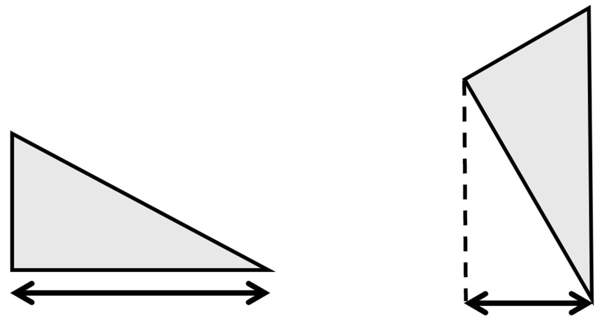
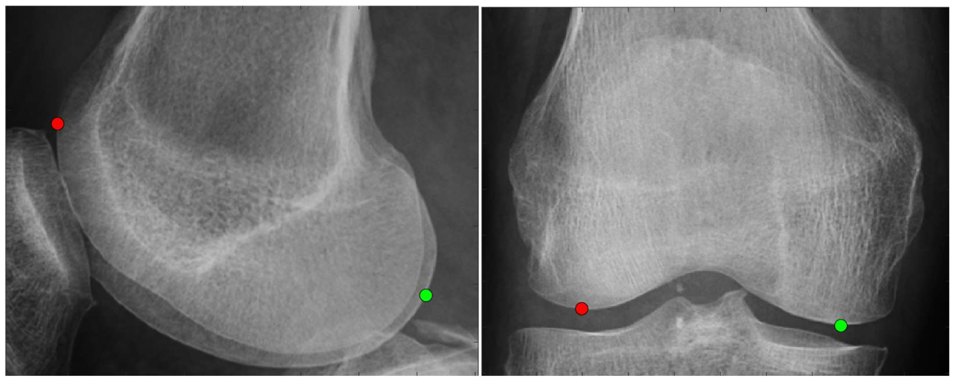
In this study, “feature points” refer to specific anatomical or contour landmarks identified on the medical images. These include manually selected or computed points along the femoral contours. “Feature values” are the numerical measurements derived from these points. To obtain feature values from medical images and 3D shape models, feature points are selected based on criteria such as the “outermost point” or “innermost point,” but as shown in Figure 3, if the 3D shape model and medical images are measured while the inclination is not consistent, an accurate model cannot be created, because incorrect feature values were obtained. Therefore, two points of the femoral condyle were selected as shown in Figure 4, and the tilts of images were adjusted so that the angles of the two points coincide in the 3D shape model and the medical image.

2.3. Acquisition of Feature Points and Feature Values from Medical Images and Shape Model

After correcting the tilts of the images, feature points were determined in both the images and the model, and feature values were calculated from those values. In this study, the following two methods of feature value acquisition were used. The size of the object on the X-ray image varies from the actual size depending on the distance between the object and the film at the time the image is taken. However, because the data used in this study did not have information when imaging, the length of the X-ray image was tentatively corrected by multiplying this length by 0.91, based on comparison with the reference model.

2.3.1. Anatomical Feature Point

First, a total of eight feature points were obtained from medical images of the sagittal and coronal planes as shown in Figure 5, and a total of five lengths, which are combinations of these points, were used as feature values, following the method used by Mohammadi et al. [15] to obtain feature values from tomographic images. Mohammadi et al. [15] proposed a method in which feature points are defined along the bone contour in 2D tomographic images by dividing a reference line into equal parts. These points are then used to generate a distance vector from a fixed reference point, which captures the shape profile of the contour. This vector is used as the feature value for matching between images and 3D models. In our study, we adapted this approach by applying it to both sagittal and coronal planes, selecting the posterior-lateral reference point, and assuming depth coordinates based on the model geometry to convert 2D information into 3D deformation input.

2.3.2. Scanning Feature Values

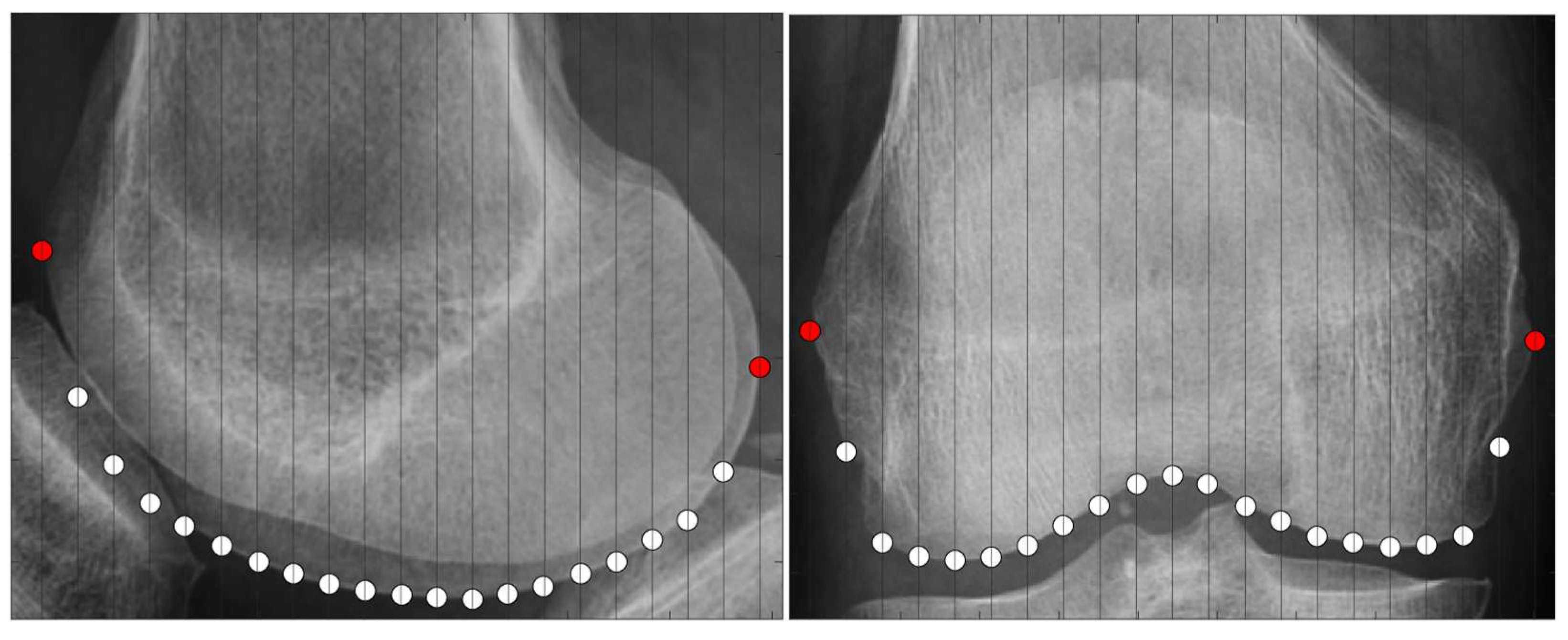
The second method acquires several points that constitute the contour line near the knee joint as feature points in both the medical images and the 3D shape model, as shown in Figure 6, and uses all their distances from the reference point as feature values. To implement this method, feature points and feature values were acquired in both the medical images and the 3D shape model according to the following procedure:
  • Select two points located at both ends.
  • Of the two points obtained in step 1, designate the point located posteriorly in the sagittal plane and laterally in the coronal plane as the reference point.
  • Draw a perpendicular line on the images that divides the two points into n equal parts.
  • Obtain the intersection of the line drawn in step 3 and the bone contour line.
  • Calculate the distances between all points and the reference point and use them as the feature values.
The above procedure was performed in both the coronal and sagittal planes and 2 × (n + 1) feature values were obtained for both the medical images and the 3D shape model. Deformations were made to match these feature values. In this study, n = 20. The reference points were defined as described above because it was considered to be most easily identifiable in both the medical images and the 3D shape model. The depth coordinates of the feature points obtained from the medical images were defined as the same as the coordinates of the relatively co-located points in the model. For scanning feature values obtained from 2D X-ray images, only the coordinates in the image plane were directly measurable. To estimate the depth coordinate, we identified the anatomically corresponding point on the surface of the base model based on its 3D contour geometry and assigned its z-coordinate to the feature point. These corresponding points, referred to as “relatively co-located,” were selected by projecting each image point onto the bone contour of the model in the same anatomical region (e.g., femoral condyle). This assumption allows for depth approximation from single-view images but may introduce errors if the depth profile of the base model differs significantly from that of the target patient.

2.4. Deformational Technique

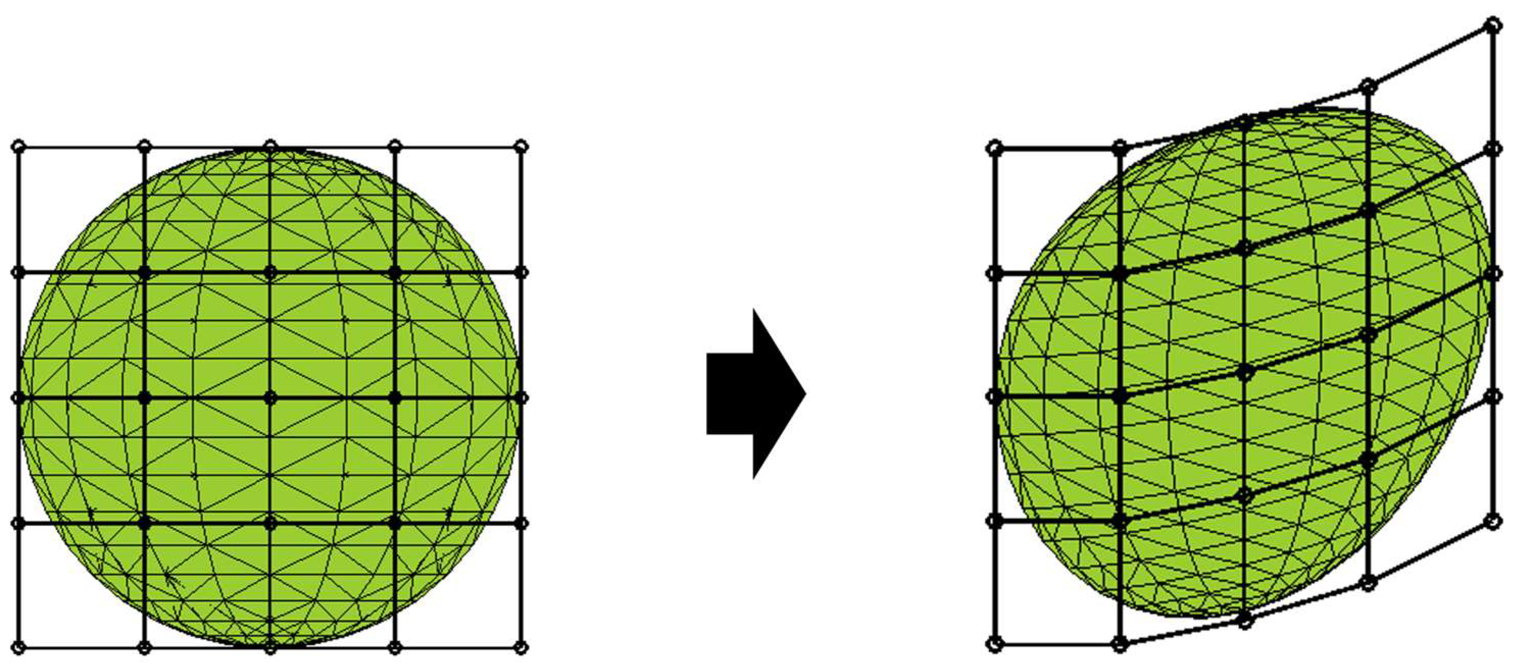
The proposed method uses the computer graphics data deformation method called FFD. Figure 7 shows a schematic diagram. The following is a description of the specific method used for FFD. First, the data to be deformed are placed in the world coordinate system, such as the sphere in Figure 7, and a rectangle is created that encloses the data to be deformed. If any vertex of the rectangle is X0 and the lengths of each side of the rectangle extending from that vertex are S , T , and U , then the value in the world coordinate system of a point X inside the rectangle is expressed by Equation (1).
X = X 0 + s S + t T + u U
where s , t , and u are the normalized numbers of node points constituting the 3D shape model, and the minimum value in the x, y, and z axes is 0 and the maximum value is 1. The coordinate system that represents the data of the shape model with this combination of ( s , t , u ) is called the FFD coordinate system. The values of s   , t , and u are obtained from the values of X using Equation (2).
s = T × U · X X 0 T × U · S t = S × U · X X 0 S × U · T u = S × T · ( X X 0 ) S × T · U
Next, control grid points are created to cover the interior of the rectangle at equal intervals. Control grid points l + 1 , m + 1 , and n + 1 are created in the x, y, and z axes, respectively, and their coordinates are expressed using Equation (3).
P i j k = X 0 + i l S + j m T + k n U
where P i j k is the i-th, j-th, and k-th control grid point in each axis direction. When the control grid point P i j k defined above is moved, the FFD coordinate system is simultaneously deformed, and the node point coordinates X F F D constituting the deformed 3D shape model are calculated using Equation (4), allowing the data representing the shape inside the control grid point to be deformed. In this deformation, an interval polynomial is used with a Bezier curve as the basis, with the control grid points as control points.
X F F D = i = 0 l j = 0 m k = 0 n B i l s B j m t B k n ( u ) P i j k  
where B is the Bernstein polynomial and is expressed by Equation (5).
B i l s = l ! i ! l i ! 1 s l i
In this study, the maximum and minimum values in the x, y, and z axes were defined as the vertices of the control grid points in the 3D shape model after coordinate transformation. A total of 243 control grid points were placed in the x, y, and z axes, that is, 9, 9, and 3, respectively.

2.5. Optimization Calculation

In this study, the amount of displacement of the control grid points used in the FFD described in the previous section was obtained using optimization calculations. The confidence region method was used as the algorithm. The amount of movement of the control grid points, which is unknown, was calculated to minimize the evaluation function in Equation (6). To define this evaluation function, we referred to the method of Mochimaru et al. [16].
E = i = 1 I j = 1 J k = 1 K   C i , j , k C i 1 , j , k D x i , j , k 2 + C i , j , k C i + 1 , j , k D x i , j , k 2 + C i , j , k C i , j 1 , k D y i , j , k 2 + C i , j , k C i , j + 1 , k D y i , j , k 2 + C i , j , k C i , j , k 1 D z i , j , k 2 + C i , j , k C i , j , k + 1 D z i , j , k 2 + w f = 1 F P o f P t f 2  
where I, J, and K are the number of grid points in the x, y, and z axes, respectively; C ( i , j , k ) are unknowns and represent the coordinates of the control grid points after the deformation; D x , D y , and D z are the distances between adjacent control grid points at the initial position in the x, y, and z axes, respectively; w is the weight; F is the number of feature values used; P o is the feature value on the 3D shape model after deformation, which is defined by C and is therefore unknown; and P t is the feature value obtained from the medical images. The first term of this evaluation function works to control grid points so the original rectangle deforms as little as possible, and the second term works to make the feature values after deformation match the acquired feature values. In this study, the weight w was set to 200 by trial and error. The value of the weighting coefficient w = 200 was selected empirically based on trial-and-error tuning to achieve a balance between deformation accuracy and shape stability. In our preliminary tests, lower values (e.g., w = 50 ) led to underfitting of the feature constraints, while significantly higher values (e.g., w = 400 ) caused unrealistic surface distortion. Although a formal sensitivity analysis was not conducted in this study, future work will include a more systematic investigation of how this parameter affects deformation quality and convergence.

2.6. Evaluation

To investigate whether FFD by the optimization calculation used in this study is appropriate as a deformation method and whether the individual adaptation method in this study is useful, an accuracy evaluation was performed based on three elements: the acquired feature values, the model after deformation, and the reference model. In the reference model, 13 cases were used, with an average of 5007 nodes, an average of 10,000 elements, and an average element size (length per side) of 2.25 mm. First, the deformed model and the reference model were aligned. In this case, the two models were first placed with some overlap manually, and then the iterative closest point algorithm was used to treat both the deformed model and the correct model as a point cloud for alignment. As an evaluation item, we checked the degree to which the feature values in the deformed model matched the feature values obtained as described in Section 2.4 to determine whether FFD is appropriate as a deformation method. To confirm this, three cases were examined, and the mean error, root mean square error (RMSE), and maximum error were used. In addition, to investigate whether the acquisition of feature values in our method is accurate, we checked the degree of agreement between the feature values in the reference model and the feature values acquired as described in Section 2.4. Finally, to investigate the degree of agreement not only in the feature values but also in the overall model shape, the “distance between a point and a surface” used in several previous studies [17,18,19] was also used in this study. Because no specific algorithm was presented in the previous studies, this study used the distance between the surfaces constituting the deformed model and the node points of the closest reference model to the surfaces to evaluate the model.
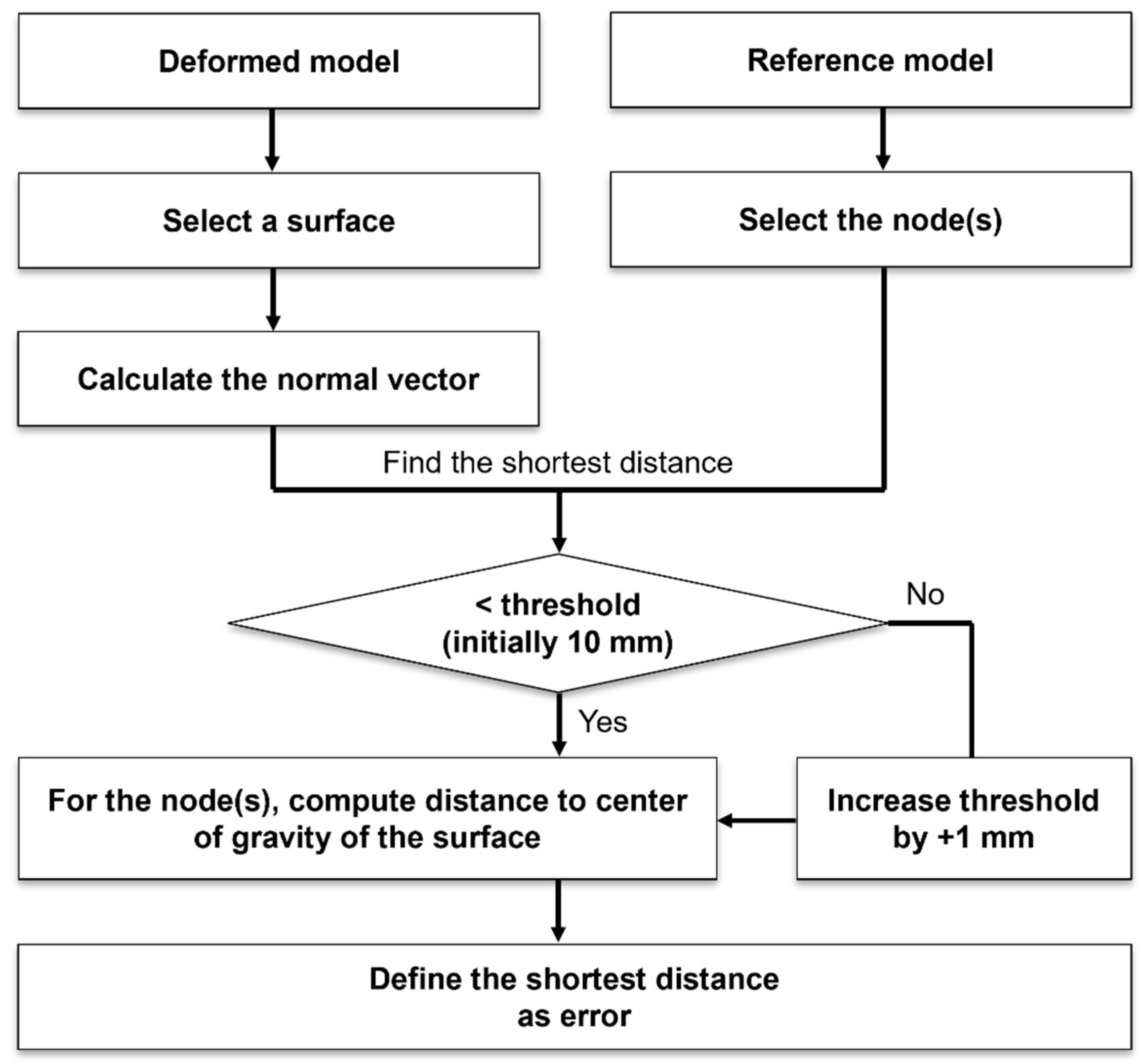
The definition of the “nearest node point” and the evaluation of the overall model shape were performed according to the following procedure (Figure 8):
  • Find the normal on any one surface of the deformed model.
  • Find the shortest distance between the normal obtained in step 1 and the node point of the reference model.
  • Find a node whose shortest distance calculated in step 2 is less than a certain threshold.
  • If there is no point below the threshold value in step 3, set the threshold value to +1 mm.
  • Find the distance between the point obtained in step 3 and the center of gravity of the surface chosen in step 1.
  • Define the point with the shortest distance obtained in step 5 as the closest node point; then, the value of the distance is the error between the model after deformation and the reference model.
  • Repeat steps 1 through 6 for all surfaces that make up the deformed model.
The mean error and maximum error were calculated from the values obtained in the above procedure and used as the evaluation scale. The threshold value used in step 3 was determined by trial and error to avoid outliers and was set at 10 mm. In addition, because this study focused on the geometry near the knee joint and did not perform active deformation near the bone axis, this portion of the bone was excluded from the evaluation. In this study, the bone axis and joint coordinate system were not preserved during the deformation process, as these structures shift along with surface geometry and cannot accurately represent joint kinematics post-deformation. Since the primary goal was to individualize bone shape using sparse imaging data, the joint coordinate system can be redefined based on the deformed geometry in subsequent biomechanical analyses. Standard surface distance metrics such as Hausdorff distance [20] were not used in this study due to differences in mesh topology and evaluation focus. Instead, we adopted a centroid-based distance measure suitable for shell-element surface models.

3. Results

3.1. Relevance of FFD

Table 1 shows the feature values acquired from medical images and the feature values of the deformed model. For all the feature values, deformation was achieved with an accuracy of less than 0.1 mm.

3.2. Comparison and Accuracy of Feature Value Acquisition Methods

Table 2 shows the feature values acquired from medical images and those from the reference model. This table shows that there is a significant difference in accuracy between the two methods of feature value acquisition.

3.3. Evaluation of the Overall Model Shape

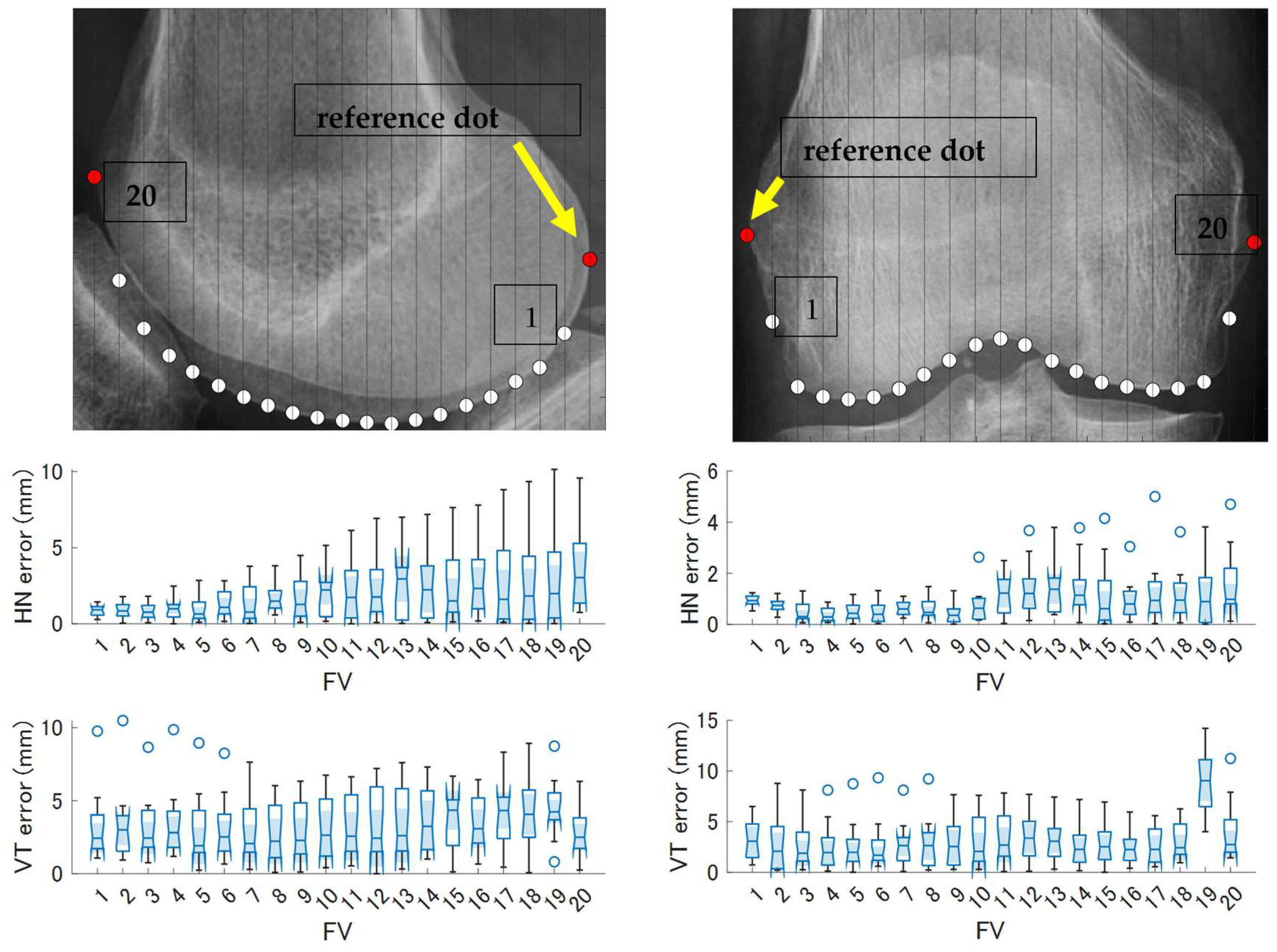
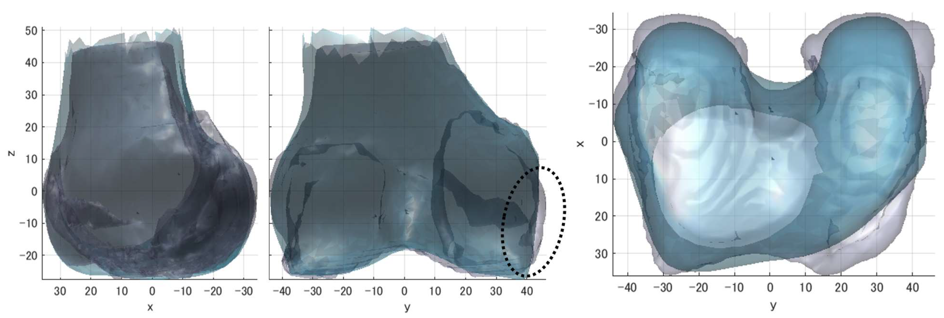
The results of the evaluation using the distances between the surfaces of the deformed model and the node points of the reference model, described at the end of Section 2.6, are shown in Table 3. The average error for the 13 cases was 1.54 mm, and the maximum error was 12.88 mm. Figure 9 shows the error for each scanning feature value used in this study. In the sagittal plane, the horizontal error increased as the distance from the reference point increased, but the median error was within about 3 mm. Vertical errors often took values between 2 mm and 5 mm throughout. In the coronal plane, horizontal errors were small throughout with rare outliers, but within 3 mm. Conversely, the median error at the 19th point in the vertical direction was 10 mm, which is very large compared to the other points. However, for all points except the 19th, the errors were similar to the others. As shown in Figure 10, the qualitative evaluation showed that the shape was roughly reproduced in the sagittal and coronal planes, but in many cases, the shape was not reproduced in the horizontal plane, where the medical images were not used.

4. Discussion

The findings of this study validate the effectiveness and practicality of the proposed deformation framework based on free-form deformation (FFD) and feature-value-based optimization. The method achieved high accuracy in matching the target feature values extracted from medical images, with mean errors of less than 0.1 mm across the test cases, as summarized in Table 1. This level of precision indicates that the optimization algorithm successfully identifies a locally optimal deformation of the generic model that reflects the target subject’s anatomical characteristics. Importantly, this performance was achieved in a fully automated manner, without the need for manual mesh editing or template fitting.
In terms of computational load, the study utilized a deformation grid comprising 243 control points (9 × 9 × 3), with feature matching targets set at five anatomical lengths and 42 scanning-derived distances. Despite the increase in feature values, the computation time remained consistently around 13 min. This suggests that the number of control grid points, rather than the number of target feature values, is the primary driver of computational complexity in this framework. This is consistent with the trends observed in previous FFD-based studies [21]. The ability to increase the number of feature values without significantly increasing computational time is a key advantage, as it allows more detailed anatomical fidelity while maintaining feasibility in routine applications.
The substantial difference in maximum error between the anatomical feature method (39.56 mm) and the scanning feature method (10.14 mm) can be attributed to the number and spatial distribution of feature constraints. The anatomical method relies on a limited number of discrete anatomical landmarks, which may not adequately capture local surface variations, especially in areas with high morphological complexity. As a result, localized deformations can become less accurate. On the other hand, the scanning feature method acquires multiple contour points along the bone outline, enabling more continuous and distributed constraints across the surface. This results in better shape conformity and helps reduce large localized deviations in the deformed model. With respect to feature acquisition strategies, the comparative evaluation revealed that anatomical feature points are prone to larger errors, especially in regions distant from the selected points. This is likely due to the sparse and discrete nature of anatomical landmarks, which may not fully constrain the deformation process in complex joint geometries. In contrast, the scanning-based method, which captures continuous contour information across sagittal and coronal planes, offers higher resolution and better constraint over the deformation process. This resulted in improved local shape reproduction, with errors mostly within 3 mm horizontally and 5 mm vertically. However, in areas with high geometric curvature or abrupt shape transitions—such as the posterior condyle—the model struggled to maintain accuracy. This is particularly evident in Figure 10, where the circled region highlights a mismatch due to under-constrained deformation caused by sparse control point density along the y-axis. With only nine points distributed across twenty-one feature values in that direction, the optimization tends to average out the error across the region, leading to shape smoothing and local deviations.
Nevertheless, the overall shape reconstruction accuracy achieved in this study is considered acceptable and comparable to previous literature. Prior works using biplanar radiographs and statistical shape models reported average errors around 1 mm and maximum errors up to 4 mm [17,18,19]. In our case, the global average surface deviation across 13 subjects was 1.54 mm, with a maximum deviation of 12.88 mm. While the peak error is higher than previous reports, it was mostly concentrated in out-of-plane regions (e.g., transverse plane) not directly constrained by X-ray-derived features. Given that our method utilizes only two simple X-ray images and a single base model, these results demonstrate favorable performance, particularly in reproducing the joint morphology of the knee, which was the focal region of this study. Although this study reported a maximum error of 12.88 mm, these deviations were confined to anatomically complex regions with high curvature, such as the intercondylar notch and posterior condyle, where feature constraints were sparse. Since the primary objective is to construct subject-specific models for biomechanical analysis—particularly musculoskeletal simulations of the knee joint incorporating cartilage and meniscus—clinical-level accuracy is not required. Rather, the model must preserve sufficient bone morphology to enable reliable reconstruction of surrounding soft tissues. We acknowledge that a maximum surface deviation of 12.88 mm, particularly in the condylar region, may affect localized outputs such as joint contact mechanics or ligament tension. However, for the intended application in subject-specific musculoskeletal or finite element modeling aimed at estimating gross joint kinematics or muscle forces, previous studies have shown that models based on approximated or generic geometries can still yield valid predictions [22,23]. Therefore, while this error level limits the method’s clinical applicability, it may still be tolerable within certain classes of biomechanical simulation.
Two primary factors likely contributed to discrepancies between the acquired feature values and the corresponding values in the reference models. First, the magnification factor in X-ray imaging depends on the relative distance between the X-ray source, subject, and detector. In this study, because the imaging conditions (such as source-to-image distance and object-to-detector distance) were not available, a uniform scale factor (0.91) was estimated and applied based on comparison with the reference model. This scaling approximation undoubtedly introduced residual errors, especially in absolute measurements. Second, although efforts were made to correct for inclination in the sagittal (flexion–extension) and coronal (adduction–abduction) directions, the internal/external rotational alignment could not be adjusted using 2D images alone. As a result, different cross-sectional planes may have been compared between the X-ray-derived features and the reference CT model, reducing correspondence accuracy. Previous studies have similarly noted unintended rotational deviations even during guided orthopedic procedures [24], underscoring the importance of rotational correction.
Several methodological limitations should also be acknowledged. First, the evaluation function used during optimization assigned uniform weights to all feature values. This assumption may be overly simplistic, as different anatomical regions likely contribute unequally to clinically relevant shape accuracy. Future work will explore adaptive weighting schemes that prioritize high-curvature areas or clinically significant zones, such as the articular surface or posterior condyles. Weight tuning could improve deformation fidelity without dramatically increasing computation time.
Second, increasing the resolution of the FFD grid does not linearly improve model accuracy. While a grid of 5 × 5 × 3 control points yielded computation times of about 2 min, increasing to 9 × 9 × 3 required roughly 12–13 min, and 13 × 13 × 3 extended processing time to over 3 h. This exponential growth limits the practical feasibility of arbitrarily increasing control point density. Moreover, even when using region-specific weighting, the dominant number of feature values in flatter regions can dilute the influence of error-prone zones. A more sophisticated strategy, such as hierarchical FFD or local patch-based refinement, may offer better accuracy–efficiency trade-offs.
Third, the mean error of 1.54 mm and the maximum error of 12.88 mm occurred primarily in regions where the femoral contour changes abruptly. These regions tend to have high geometric complexity and are inherently irregular, with significant inter-individual anatomical variation. Due to the smoothing nature of the FFD algorithm during optimization, local details in these high-curvature areas are often averaged out, resulting in visible discrepancies between the deformed model and the actual image-based contours. Additionally, the absence of out-of-plane constraints in the FFD process exacerbates the mismatch. We acknowledge that these regions represent a current limitation of the method and suggest that future improvements could include adaptive control point density and localized weighting schemes to better preserve such complex geometries. Although a mean surface error of 1.54 mm may be sufficient for biomechanical modeling and general shape analysis, this level of accuracy may still be insufficient for clinical applications that require sub-millimeter precision, such as implant design or surgical navigation. Moreover, this study required manual selection of anatomical and contour-based feature points from 2D X-ray images. We acknowledge that this step may introduce interoperator variability. To enhance reproducibility and scalability in clinical settings, future work should include a reproducibility study to quantify both intra- and inter-operator differences. Furthermore, we are currently exploring semi-automated approaches using edge detection and landmark identification algorithms to reduce human error and improve the consistency of feature extraction. Although this study focused primarily on the development and accuracy validation of the shape estimation method, we acknowledge that demonstrating a practical application, such as joint kinematics analysis or load estimation, would further support the method’s utility. Due to scope limitations, such an application was not included in the current work. However, we are currently integrating the generated models into a musculoskeletal simulation framework to evaluate joint range of motion and contact mechanics, and we plan to present these results in a follow-up study.
Although this method is intended to reconstruct femoral shape from low-cost X-ray images, validation in this study was performed using models reconstructed from CT data. This choice was made because CT-derived models offer accurate and complete 3D geometries, which are necessary to serve as the ground truth in evaluating the accuracy of the deformation and matching process. Since 2D X-ray images cannot directly provide true 3D anatomical structure, CT-based validation allows us to objectively quantify the error in the proposed method. Nevertheless, we acknowledge the importance of validating the method on actual clinical X-ray datasets and we plan to incorporate this in future work to ensure its clinical applicability. Additionally, this study included 13 cases, which is a relatively small sample size. Although the results showed acceptable accuracy, further validation with a larger and more diverse dataset is necessary to confirm generalizability.
A key limitation of the current approach is the assumption that depth coordinates of feature points are inherited from a single base model. While we expect this to introduce shape deviations, particularly in regions with high anterior–posterior variability, a detailed quantitative assessment is difficult at this stage due to lack of reference 3D data. Future work will aim to reduce this limitation through statistical modeling or multi-template approaches.
The evaluation in this study was based on distances measured at the barycentres of shell elements, consistent with the locations used for deformation constraints. While this approach ensures internal consistency, it limits direct comparison with previous studies that employ standard metrics such as Hausdorff distance [20] or mean surface error. Future work will aim to incorporate these established metrics to improve comparability and rigor.
Finally, the inability to correct for internal/external rotation remains a structural limitation of 2D-based modeling. To achieve full alignment between image-derived features and 3D geometry, it is necessary to either control the imaging orientation during acquisition or integrate a 2D–3D registration process [24]. In this study, such alignment was not possible, especially given that a statistical shape model was not employed. As a result, the base model and deformation targets may have significant intrinsic variation, particularly in transverse orientations.
Despite these limitations, the proposed approach offers a promising, low-cost alternative for generating individualized skeletal models using minimal imaging data. By avoiding the need for volumetric imaging or statistical shape databases, this method broadens access to patient-specific modeling in both research and clinical contexts.

5. Conclusions

In this study, we proposed a method to individually fit a 3D shape model of the knee joint by using only one 3D shape model as a base and deforming it using FFD and feature values acquired from two medical images. The accuracy of the deformation was evaluated for 13 cases, comprising 3 cases of CT data published by the University of Denver and 10 cases provided by Akita Hospital, after deformation using the method of this study. Although the agreement between the feature values after deformation and the feature values acquired from medical images was high for models using anatomical feature points, the scanning feature value acquisition was better for the agreement with the feature values of the reference model and for the overall shape agreement evaluation using points and surfaces. A mean error of 1.54 mm and a maximum error of 12.88 mm were obtained for the 13 cases. By using automated FFD with optimization computation as the deformation method, the burden on the model creator can be minimized to just extracting feature values from the medical images. Although image rotation may cause some errors, and a solution to this problem has not yet been determined, we believe that our method is useful.

Author Contributions

Conceptualization, S.W., K.H. and K.Y.; methodology, K.H. and I.F.; software, S.W.; validation, I.F.; formal analysis, I.F.; investigation, I.F.; resources, K.H.; data curation, I.F. and K.H.; writing—original draft preparation, I.F.; writing—review and editing, K.H. and S.W.; visualization, I.F.; supervision, K.H.; project administration, K.H.; funding acquisition, K.H. All authors have read and agreed to the published version of the manuscript.

Funding

This research received no external funding.

Institutional Review Board Statement

The study was conducted according to the guidelines of the Declaration of Helsinki, and approved by the research ethics committee of the Tokyo Metropolitan University (protocol code: H5-154 and date of approval: 11 June 2023).

Data Availability Statement

The data presented in this study are available on request from the corresponding author.

Conflicts of Interest

The authors declare no conflicts of interest.

References

  1. Mercader, A.; Rottinger, T.; Bigdeli, A.; Luth, T.C.; Rottinger, H. A patient-specific 3D model of the knee to compare the femoral rollback before and after total knee arthroplasty (TKA). J. Exp. Orthop. 2021, 8, 2. [Google Scholar] [CrossRef] [PubMed]
  2. Otomaru, I.; Nakamoto, M.; Takao, M.; Sugano, N.; Kagiyama, Y.; Yoshikawa, H.; Tada, Y.; Sato, Y. Automated preoperative planning of femoral component for total hip arthroplasty (THA) from 3D CT images. JBSE 2008, 3, 478–489. [Google Scholar] [CrossRef]
  3. Wang, S.; Hase, K.; Ota, S. Development of a lower limb finite element musculoskeletal gait simulation framework driven solely by inertial measurement unit sensors. Biomechanics 2021, 1, 293–306. [Google Scholar] [CrossRef]
  4. Wang, S.; Hase, K.; Ota, S. A computationally efficient lower limb finite element musculoskeletal framework directly driven solely by inertial measurement unit sensors. J. Biomech. Eng. 2022, 144, 051011. [Google Scholar] [CrossRef] [PubMed]
  5. Kalra, K.M.; Maher, M.M.; Rizzo, S.; Kanarek, D.; Shephard, O.J. Radiation exposure from chest CT: Issues and strategies. J. Korean Med. Sci. 2004, 19, 159–166. [Google Scholar] [CrossRef]
  6. Meulepas, J.M.; Ronckers, C.M.; Smets, A.M.J.B.; Nievelstein, R.A.J.; Gradowska, P.; Lee, C.; Jahnen, A.; van Straten, M.; de Wit, M.Y.; Zonnenberg, B.; et al. Radiation exposure from pediatric CT scans and subsequent cancer risk in the Netherlands. JNCI J. Natl. Cancer Inst. 2019, 111, 256–263. [Google Scholar] [CrossRef]
  7. Shellock, F.G.; Crues, J.V. MR procedures: Biologic effects, safety, and patient care. Radiology 2004, 232, 635–652. [Google Scholar] [CrossRef]
  8. Inaguma, K.; Kotani, T.; Kishida, S.; Sakuma, T.; Ueno, K.; Iijima, Y.; Kajiwara, D.; Okuyama, K.; Sakashita, K.; Okuwaki, S.; et al. Medical accidents related to ferromagnetic objects brought into the MRI Room: Analysis of the national multicenter database by orthopedic surgeons. SSRR 2023, 7, 96–102. [Google Scholar] [CrossRef]
  9. Reyes-Santias, F.; Garcia-Garcia, C.; Aibar-Guzman, B.; Garcia-Campos, A.; Cordova-Arevalo, O.; Mendoza-Pintos, M.; Cinza-Sanjurjo, S.; Portela-Romero, M.; Mazon-Ramos, P.; Gonzalez-Juanatey, J.R. Cost analysis of magnetic resonance imaging and computed tomography in Cardiology: A case study of a university hospital complex in the euro region. Healthcare 2023, 11, 2084. [Google Scholar] [CrossRef]
  10. Bhalodia, R.; Elhabian, S.; Adams, J.; Tao, W.; Kavan, L.; Whitaker, R. Deepssm: A blueprint for Image-to-Shape deep learning models. Med. Image Anal. 2024, 91, 103034. [Google Scholar] [CrossRef]
  11. Kurazume, R.; Nakamura, K.; Okada, T.; Sato, Y.; Sugano, N.; Koyama, T.; Iwashita, Y.; Hasegawa, T. 3D reconstruction of a femoral shape using a parametric model and two 2D fluoroscopic images. Comput. Vision Image Underst. 2009, 113, 202–211. [Google Scholar] [CrossRef]
  12. Sederberg, T.W.; Parry, S.R. Free-form deformation of solid geometric models. ACM SIGGRAPH Comput. Graph. 1986, 20, 151–160. [Google Scholar] [CrossRef]
  13. Jack, D.; Pontes, J.K.; Sridharan, S.; Fookes, C.; Shirazi, S.; Maire, F.; Eriksson, A. Learning Free-Form deformations for 3D object reconstruction. Lect. Notes Comput. Sci. 2018, 11362, 317–333. [Google Scholar]
  14. Modenese, L.; Renault, J. Automatic generation of personalised skeletal models of the lower limb from Three-Dimensional bone geometries. J. Biomech. 2021, 116, 110186. [Google Scholar] [CrossRef]
  15. Mohammadi, A.; Myller, K.A.H.; Tanska, P.; Hirvasniemi, J.; Saarakkala, S.; Toyras, J.; Korhonen, R.K.; Mononen, M.E. Rapid CT-based estimation of articular cartilage biomechanics in the knee joint without cartilage segmentation. Ann. Biomed. Eng. 2020, 48, 2965–2975. [Google Scholar] [CrossRef]
  16. Mochimaru, M.; Kouchi, M.; Fukui, Y.; Tsutsumi, E. Classification of 3D foot shape based on Inter-shape distance using the FFD method. Jpn. J. Ergon. 1997, 33, 229–234. [Google Scholar] [CrossRef]
  17. Laporte, S.; Skalli, W.; de Guise, J.A.; Lavaste, F.; Mitton, D. A biplanar reconstruction method based on 2D and 3D Contours: Application to the distal femur. Comput. Methods Biomech. Biomed. Eng. 2003, 6, 1–6. [Google Scholar] [CrossRef] [PubMed]
  18. Mitton, D.; Landry, C.; Veron, S.; Skalli, W.; Lavaste, F.; de Guise, J.A. 3D reconstruction method from biplanar radiography using non-stereocorresponding points and elastic deformable meshes. Med. Biol. Eng. Comput. 2000, 38, 133–139. [Google Scholar] [CrossRef] [PubMed]
  19. Mitulescu, A.; Semaan, I.; de Guise, J.A.; Leborgne, P.; Adamsbaum, C.; Skalli, W. Validation of the non-stereo corresponding points stereoradiographic 3D reconstruction technique. Med. Biol. Eng. Comput. 2001, 39, 152–158. [Google Scholar] [CrossRef]
  20. Huttenlocher, D.P.; Klanderman, G.A.; Rucklidge, W.J. Comparing images using the Hausdorff distance. IEEE Trans. Pattern Anal. Mach. Intell. 1993, 15, 850–863. [Google Scholar] [CrossRef]
  21. Baka, N.; Kaptein, B.L.; de Bruijne, M.; van Walsum, T.; Gihphart, J.E.; Niessen, W.J.; Lelieveldt, B.P.F. 2D-3D shape reconstruction of the distal femur from stereo X-ray imaging using statistical shape models. Med. Image Anal. 2011, 15, 840–850. [Google Scholar] [CrossRef]
  22. Marra, M.A.; Vanheule, V.; Fluit, R.; Koopman, B.H.F.J.M.; Rasmussen, J.; Verdonschot, N.; Andersen, M.S. A subject-specific musculoskeletal modeling framework to predict in vivo mechanics of total knee arthroplasty. J. Biomech. Eng. 2015, 137, 020904. [Google Scholar] [CrossRef] [PubMed]
  23. Lerner, Z.F.; Demers, M.S.; Delp, S.L.; Browning, R.C. How tibiofemoral alignment and contact locations affect predictions of medial and lateral tibiofemoral contact forces. J. Biomech. 2015, 48, 644–650. [Google Scholar] [CrossRef] [PubMed]
  24. Okamoto, S.; Mizu-uchi, H.; Okazaki, K.; Hamai, S.; Tashiro, Y.; Nakahara, H.; Iwamoto, Y. Two-dimensional planning can result in internal rotation of the femoral component in total knee arthroplasty. Knee Surg. Sports Traumatol. Arthrosc. 2014, 24, 229–235. [Google Scholar] [CrossRef] [PubMed]
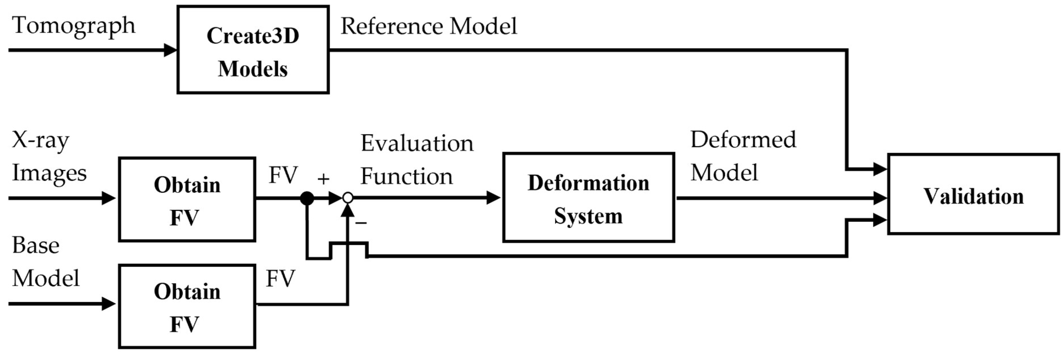
Figure 1. Overview of the processing flow in this study. The deformation system involves an optimization calculation. Validation is performed using not only the 3D model but also feature values from X-ray images, which are deformation criteria. FVs = feature values.
Biomechanics 05 00063 g001
Figure 2. Estimation of the anatomical feature points of a femur using STAPLE, one of the MATLAB toolboxes.
Biomechanics 05 00063 g002
Figure 3. Measured results for distances between the left and right “outermost points” at different tilts.
Biomechanics 05 00063 g003
Figure 4. Acquisition points for tilt adjustment; the image is modified so that the angle between the line connecting the two dots and the horizontal line matches a similar angle on the model.
Biomechanics 05 00063 g004
Figure 5. Diagram of the first feature acquisition method. Eight points represent anatomical feature points, and the five yellow lines represent feature values obtained from the combination of these points.
Biomechanics 05 00063 g005
Figure 6. Schematic diagram of scanning feature values. The dots at both ends are selected, a vertical line is drawn between them dividing them into n equal parts, and the intersection of the line and the contour line of the femur is obtained. For the sagittal plane, the rightmost dot is used as the reference point, and for the coronal plane, the leftmost point is used because this image is of the right leg.
Biomechanics 05 00063 g006
Figure 7. Schematic diagram of FFD. The sphere inside the lattice grid can be deformed by the deformation of the control lattice grid, which consists of dots and solid lines.
Biomechanics 05 00063 g007
Figure 8. The processing flow of the definition of the “nearest node point” and the evaluation of the overall model shape.
Biomechanics 05 00063 g008
Figure 9. Error with respect to the reference model for each scanning feature value (FV). The arrows on the medical images are the reference points for each feature value in the sagittal and coronal planes, and the numbers correspond to the FV in the box-and-whisker diagram. The upper boxplots show the horizontal (HN) error for each point, and the bottom boxplots show the vertical (VT) error for each point.
Biomechanics 05 00063 g009
Figure 10. One example of the deformation results. From left to right: sagittal plane, frontal plane, and horizontal plane. The gray model is the reference model, and the light blue model is the deformed model. The circled area is the area where the error was often large.
Biomechanics 05 00063 g010
Table 1. Results of determining the error between the acquired feature values and the feature values of the deformed model for the three cases (mean error, RMSE, and maximum error in mm).
Error123Global
Mean0.0800.1240.0550.087
RMSE0.1280.1680.0690.122
Max.0.2780.2720.1150.278
Table 2. Errors between the feature values acquired from the medical images and the feature values in the reference model (mean error, RMSE, and maximum error in mm). The anatomical errors concern the five feature values presented in Section 2.3.1. The scanning error relates to the 21 feature values in the sagittal and coronal planes shown in Section 2.3.2, and is further divided into horizontal and vertical values (HN = horizontal, VT = vertical).
Anatomical
123
Error Global
Mean7.0710.223.757.02
RMSE9.0817.964.7410.60
Max18.0239.568.2139.56
Scanning
123
CoronalSagittalCoronalSagittalCoronalSagittal
ErrorHNVYHNVTHNVTHNVTHNVTHNVTGlobal
Mean0.633.101.492.090.783.762.064.980.603.814.943.222.62
RMSE0.803.721.862.950.984.212.605.250.774.135.973.453.06
Max.1.628.703.226.731.908.094.107.011.555.8810.145.2110.14
Table 3. Distance between a surface in the deformed model and a point in the reference model (mean and maximum errors in mm).
Error12345678910111213Global
Mean0.530.180.361.431.841.172.311.921.881.663.131.562.051.54
Max.3.606.786.209.5510.977.5812.8810.4511.999.908.366.216.2612.88
Disclaimer/Publisher’s Note: The statements, opinions and data contained in all publications are solely those of the individual author(s) and contributor(s) and not of MDPI and/or the editor(s). MDPI and/or the editor(s) disclaim responsibility for any injury to people or property resulting from any ideas, methods, instructions or products referred to in the content.