Involuntary Breathing Movement Pattern Recognition and Classification via Force-Based Sensors

Abstract

The study presents a novel scheme that recognizes and classifies different sub-phases within the involuntary breathing movement (IBM) phase during breath-holding (BH). We collected force data from eight recreational divers until the conventional breakpoint (CB). They were in supine positions on force plates. We segmented their data into no-movement (NM) phases, i.e., the easy phase (EP) and IBM phase (comprising several events or sub-phases of IBM). Acceleration and jerk were estimated from the data to quantify the IBMs, and phase portraits were developed to select and extract specific features. K means clustering was performed on these features to recognize different sub-phases within the IBM phase. We found five–six optimal clusters separating different sub-phases within the IBM phase. These clusters separating different sub-phases have physiological relevance to internal struggles and were labeled as classes for classification using support vector machine (SVM), naive Bayes (NB), decision tree (DT), and K-nearest neighbor (K-NN). In comparison with no feature selection and extraction, we found that our phase portrait method of feature selection and extraction had low computational costs and high robustness of 96–99% accuracy.

1. Introduction

Involuntary physiological responses are present in biological systems that activate when life-threatening situations arise. The prolonged contractions of the diaphragm and external intercostal muscle during breath-holding (BH) result in one such response. Prolonged contraction and hypercapnia during BH activate chemoreceptors [1,2]. The receptors reaching the sensory cortex generate a dyspnea signal, which is crucial for the initiation of breathing [3,4]. However, humans extend BH through phasic involuntary diaphragmatic contractions, especially under certain circumstances, such as free diving [5].

The question is: can sensors detect movement patterns associated with these involuntary contractions? This question is crucial for abnormal breathing detection, and the answer is in the duration and strength of involuntary muscle contractions during the struggle phase (SP). SP is a phase in which involuntary breathing movements (IBMs) appear due to deep muscle involuntary contractions. Thus, invasive methods, such as pressure transducer-based catheters, can capture them [6]; non-invasive methods, such as surface electromyography (sEMG) and force plates during strong contractions associated with IBM, can also be applicable [4,7,8]. IBM starts with the physiological breakpoint (PB, the point where the first IBM appears) and ends with the conventional breakpoint (CB, the point where breathing is resumed voluntarily) [7]. The IBMs are periodic and very subtle and are controlled autonomously during SP [4]. Thus, rhythmic varying patterns of IBMs associated with involuntary periodic contractions can be acquired using force-based non-invasive methods.

Previous studies used simple computational models to detect phases during BH (onset and end offset of the IBM phase) [6]. However, the IBM phase is more complex than just onset and end offset. IBMs in SP are rapid continuous movements of varying magnitudes. Previous studies have shown complex varying phases of IBMs, as IBM amplitudes and frequencies continued increasing until the CB [9,10]. Thus, using a simple model, it is hard to detect patterns or sub-phases in a movement of such nature. Moreover, the current literature does not present methods to recognize such sub-phases within the IBM phase. Therefore, methods emphasizing detecting patterns or sub-phases within the IBM phase are of importance in clinical science and should be developed. Hence, the goal of our study was to design such a method. We refer to the IBM phase as several events or patterns of IBMs during the SP.

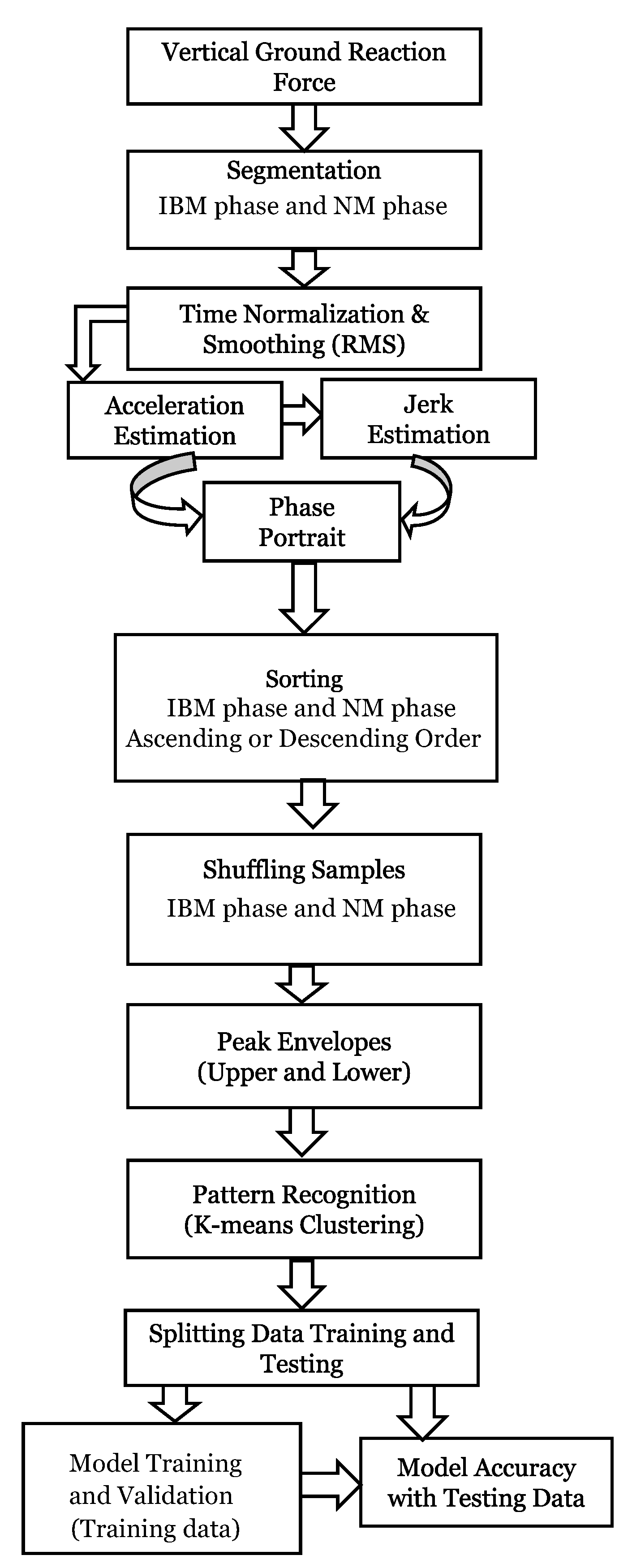
In this study, we present a novel scheme (shown in Figure 1) that can recognize different sub-phases within the IBM phase during BH, and classify them accordingly. The force sensors were used to capture kinetics associated with IBMs as they comprise mechanical components [4]. We did not use force data directly for the categorization because kinematic patterns of rapid movements can be quantified nicely through jerk and acceleration. Hence, rapid movements related to involuntary contractions during BH were estimated using acceleration and jerk. These outputs were later used as features for pattern recognition and classification of IBM sub-phases.

2. Materials and Methods

The IRB review board of Colorado Mesa University has approved this study. In this study, we recruited eight healthy participants who were recreational divers. Divers generally have higher lung capacities and better control of their breathing due to years of intense training. This makes them a better fit for our study. The demographic data of participants recruited in our study are listed in

Table 1. Demographic data of participants.

Participant ID	Sex	Age${}_{\mathit{u}}$	Height${}_{\mathit{v}}$	Mass${}_{\mathit{w}}$	Experience${}_{\mathit{u}}$
P1	Male	20 s	183.5	87.5	6
P2	Female	20 s	174.5	72.0	6
P3	Male	20 s	183.0	78.0	15
P4	Male	20 s	171.0	67.0	1
P5	Female	20 s	164.0	63.5	12
P6	Male	20 s	190.0	79.0	2
P7	Male	20 s	174.5	89.5	3
P8	Male	20 s	189.0	114.0	5
ine Avg ± Sd			178.7 ± 9.1	81.3 ± 16.0	6.25 ± 4.9

Units:- u years, v centimeters, w kilograms, u years, Avg is average, Sd is standard deviation.

.

2.1. Experimental Design

Data collection for each participant involved a single visit to our lab. On the visit, signed consent was obtained, and data regarding the participant’s age, gender, height, weight, and years of experience were recorded, as shown in Table 1. Participants were also instructed to avoid eating, drinking, and exercising two hours before the data collection. Two AMTI force plates were used to acquire the data from the participants at a sampling rate of 1 KHz. The force plates contained load cells that could measure the force associated with movement. We asked the participant to lay in a supine position on the force plates. Participants were in static postures, covering the force plate surfaces mostly with their upper and middle backs. Moreover, to maintain a comfortable posture during data collection, a cushion and a rolled-up pad were positioned under each participant’s head and knees.

We introduced a warm-up session in three steps. In the first step, participants breathed normally (relaxation) for five minutes followed by a minute of BH. In the second step, the relaxation period was reduced to two minutes, and the BH phase was incremented by an additional sixty seconds from the previous step. In the third step, participants relaxed again, followed by three minutes of BH.

Prior to data collection, participants were given enough relaxation periods. For data collection, they were asked to hold their breath as long as they could. The data were recorded from the participant’s first inhalation (starting BH) to voluntary exhalation (ending BH). The participants were asked to lay down after data collection until lightheaded subsided.

2.2. Data Analysis

We used R programming software (R 4.2.0) for signal processing and data analysis. The supine posture and the muscle spasm exerted force vertically, resulting in the appearance of IBMs (primarily in the vertical direction) (z). Hence, force plates were used to capture this biological phenomenon, and the force data in the vertical direction (vertical ground reaction force) were analyzed.

The IBMs appeared later during the BH. Thus, we segmented vertical ground reaction force data into the no-movement (NM) phase and IBM phase through visual inspections. The NM phase data consisted mostly of baseline noise. The IBM phase consisted of several IBM events. Hence, it was easy to isolate these two phases with visual inspections.

The segmented data were time-normalized (spline interpolation) to 10,000 time points for the IBM phase (10,000 × 1) and NM phase (10,000 × 1) for each participant (10,000 × 1 × 8). Later, the segmented data were smoothed using a root mean square function with a window size of 50 ms. The IBM and NM data (time normalized and smoothed) were combined to form a processed vertical ground reaction force data vector (20,000 × 1 × 8).

2.3. Acceleration and Jerk Estimation

Participants experienced no significant center of mass ($COM$) displacement of other body segments due to their static postures. Therefore, we assumed full body $COM$ in the chest; acceleration ($\overrightarrow{a}$) and jerk ($\overrightarrow{j}$) of the IBM phase were estimated from the processed vertical ground reaction force ($F_z$), as shown below.

$${\overrightarrow{F_z}}^{20000\times 1}={\overrightarrow{F_a}}^{20000\times 1}+W$$

(1)

$${\overrightarrow{F_z}}^{20000\times 1}=m\times (\overrightarrow{a}{}_{COM}^{20000\times 1}+g)$$

(2)

$${\overrightarrow{a_z}}^{20000\times 1}=\frac{{\overrightarrow{F_z}}^{20000\times 1}}{m}-g$$

(3)

$${\overrightarrow{j_z}}^{20000\times 1}={\frac{\delta \overrightarrow{a_z}}{\delta t}}^{20000\times 1}$$

(4)

$\overrightarrow{F_a}$ is the dynamic force data vector due to the accelerating center of mass (${\overrightarrow{a}}_{COM}$), W is the weight of the participant’s chest, m is the mass of the participant’s chest. The participant’s chest mass is calculated from the thorax percentage contribution to full-body mass [11], and g is the acceleration due to gravity. The superscript displays the dimension of the data vector for a single participant in Equations (1)–(4).

2.4. Phase Portraits of Jerk and Acceleration

A phase portrait ($\overrightarrow{P}$) is a geometric representation of the dynamic trajectories in the phase plane [12]. The $\overrightarrow{a}$ and $\overrightarrow{j}$ data were used to develop phase portraits for feature selection and extraction. The phase portraits yielded phases that overlapped between the IBM and NM phases. Thus, developing phase portraits were crucial to remove phases and frequencies that overlapped between the NM and IBM phases. Feature selection and extraction through phase portraits may be useful to enhance the performance (accuracy, computation, robustness) of our pattern recognition and detection scheme.

$$\overrightarrow{P}{}^{20000\times 2}=(x=\overrightarrow{a},y=\overrightarrow{j})$$

(5)

We first separated the data points overlapping between the IBM and NM phases by sorting the values of $\overrightarrow{a}$ and $\overrightarrow{j}$ in descending/ascending order from the phase portraits. These samples of $\overrightarrow{a}$ and $\overrightarrow{j}$ were then shuffled randomly and independently so that the features represented unbiased populations of the data. Furthermore, peak envelopes, lower (${\overrightarrow{a}}_{RMS\left(u\right)}$, ${\overrightarrow{j}}_{RMS\left(u\right)}$), and upper envelopes (${\overrightarrow{a}}_{RMS\left(l\right)}$, ${\overrightarrow{j}}_{RMS\left(l\right)}$) were extracted. These features were finally used for unsupervised and supervised learning.

2.5. Unsupervised Learning

We performed unsupervised learning to recognize similarities and/or dissimilarities between the IBM and NM phases and to recognize specific patterns/sub-phases/groups within the IBM phase. These groups were labeled as different classes for classification.

The K means cluster analysis was implemented on the extracted features (${\overrightarrow{a}}_{RMS\left(u\right)}$, ${\overrightarrow{j}}_{RMS\left(u\right)}$, ${\overrightarrow{a}}_{RMS\left(l\right)}$, ${\overrightarrow{j}}_{RMS\left(l\right)}$) as an unsupervised learning algorithm. The K means clustering algorithm groups the data points within these features based on their similarity into clusters.

2.6. Statistical Analysis

To test the normality, we performed the Kolmogorov–Smirnov test. The type (parametric or non-parametric) of test to compare the difference between the IBM and NM phases was based on the rejection of the null hypothesis. We considered a significance value of p < 0.05 to reject the null hypothesis [13].

Additionally, the equality of variance between the NM and IBM phases was tested with Levene’s test [14]. The Wilcoxon signed rank paired test was used to compare the median of the NM and IBM phase [15]. Violin and box plots were used to display the distribution, mean, and standard deviation of the data.

2.7. Supervised Learning

A supervised learning approach was implemented to isolate the onset of different sub-phases of IBMs with a classifier. We developed a classification model with training data that made no assumption about the normality of data. We used support vector machine (SVM), naive Bayes (NB), decision tree (DT), and K-nearest neighbor (K-NN) as classifiers.

The features that were grouped into different clusters (NM phase and different IBM sub-phases) are labeled as different classes for supervised learning. Furthermore, these labeled features were split into a ratio of 75:25 for training ($\overrightarrow{a}{}_{RMS\left(u\right)}^{15000\times 1}$, $\overrightarrow{j}{}_{RMS\left(u\right)}^{15000\times 1}$, $\overrightarrow{a}{}_{RMS\left(l\right)}^{15000\times 1}$, $\overrightarrow{j}{}_{RMS\left(l\right)}^{15000\times 1}$) and testing ($\overrightarrow{a}{}_{RMS\left(u\right)}^{5000\times 1}$, $\overrightarrow{j}{}_{RMS\left(u\right)}^{5000\times 1}$, $\overrightarrow{a}{}_{RMS\left(l\right)}^{5000\times 1}$, $\overrightarrow{j}{}_{RMS\left(l\right)}^{5000\times 1}$) data. The training data were used to train the classification model, and the test data were used to evaluate the accuracy of the model. We also used the K-fold cross (K = 10) validation procedure to validate our training model before evaluating its accuracy with testing data.

3. Results

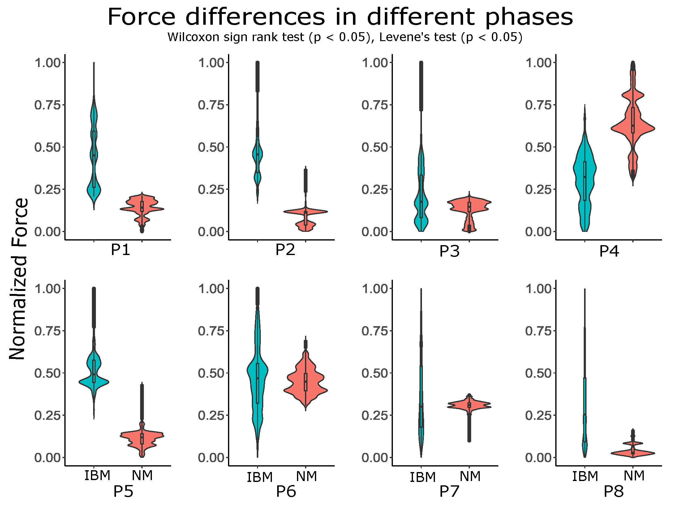
3.1. IBM Phase vs. NM Phase

We first tested whether the IBMs were present in the vertical ground reaction force, and were detectable through test statistics. Hence, we used nonparametric tests after testing the distribution of data. We found that vertical ground reaction force data were statistically significant (p≤ 0.05, Wilcoxon signed-rank paired test) between the IBM and NM phases. The force amplitude’s median values were different between the IBM and NM phases, as shown in Figure 2.

Moreover, statistically significant differences (p≤ 0.05, Levene’s test) in the variances of the ground reaction forces between the NM and IBM phases were present for all participants. Figure 2 shows the distribution of the vertical ground reaction force data for all of the participants.

The high variance during the IBM phase was due to a periodic signal output of varying amplitude. Hence, the IBMs of varying magnitudes were present in the force data and were detected using an appropriate statistical measure.

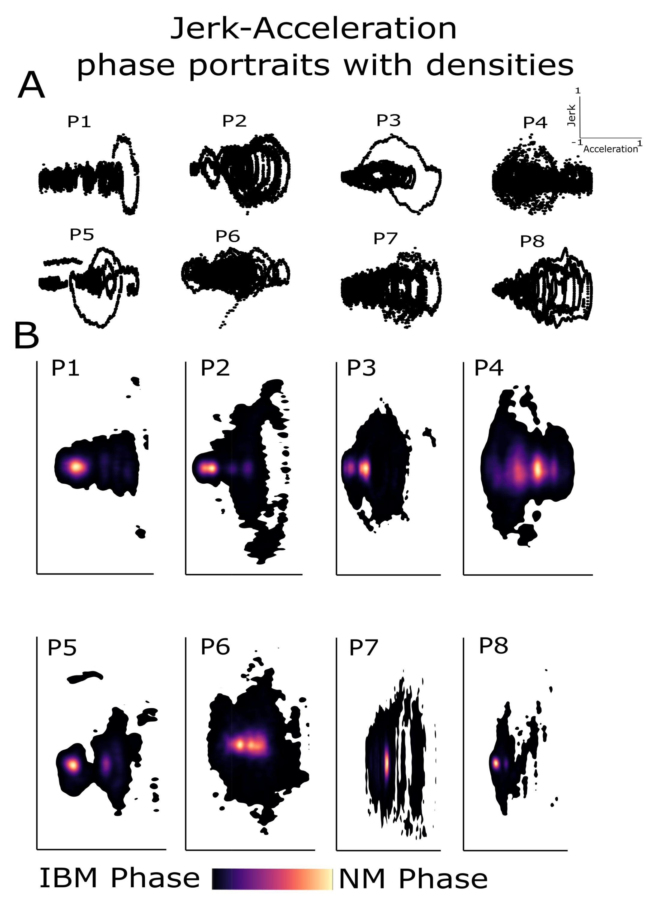
3.2. Phase Portraits of Jerk and Acceleration

The phase portraits generated from the estimated $\overrightarrow{a}$ and $\overrightarrow{j}$ were then used for feature selection and extraction. We found clear isolation between the IBM phase and NM phase from the phase portraits and their density plot, as shown in Figure 3.

The data points for the NM phase were concentrated at a specific region of less magnitude around the baseline signal. The data density was also high in this region as shown in Figure 3. Thus, the BH data were mostly composed of baseline noise associated with the NM phase.

The IBM phase concentrically surrounded the NM phase area. These concentric circles represent the regions of low, moderate, and high magnitude of $\overrightarrow{a}$ and $\overrightarrow{j}$ as shown in Figure 3. These different regions within the IBM phase suggest different sub-phases or patterns within the IBM phase. In addition, the circular shape of the phase portrait suggests the presence of some rhythmic patterns of IBMs.

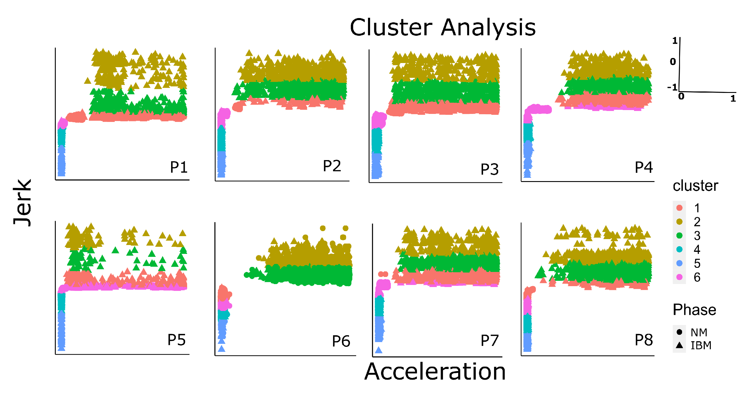
3.3. Clustering

The goal of clustering is to identify sub-phases within the IBM phase. However, we first determined the optimal number of clusters (K) that needed to be defined in the K means algorithm. We found that based on total withinness, five to six clusters were optimal for the goodness of clustering across most participants.

We then tested (through clustering) whether the IBM phase was a biological phenomenon comprising varying magnitudes of $\overrightarrow{a}$ and $\overrightarrow{j}$. We extracted peak minima and maxima values of the NM and IBM phases (sliding window = 25 samples) from the phase portraits before feeding them to K means algorithm. The cluster analysis displays clear isolation between the NM and IBM phases. Moreover, it also shows the separation of sub-phases within the IBM phase.

The cluster analysis shows that clusters 1 and 6 consist of the NM phase and few IBM data points. The centroid of these clusters was toward the point of origin (0,0) and ($\overrightarrow{a},0$), suggesting an overlap between the NM and IBM phases due to no activity. The values slightly above (0,0) for $\overrightarrow{a}$ and $\overrightarrow{j}$ in cluster 1 and 6 suggest IBM onset. Moreover, the constant $\overrightarrow{a}$ of higher magnitude was also grouped in clusters 1 and 6.

Clusters 2, 3, 4, and 5 mainly represent the IBM phase. The centroid of clusters 2, 3 4, and 5 showed varying degrees of $\overrightarrow{a}$ and $\overrightarrow{j}$ during the IBM phase, as shown in Figure 4. These clusters explained phases of $\overrightarrow{a}$ and $\overrightarrow{j}$ with (high, high), (high, moderate), (moderate, high), and (moderate, moderate) magnitudes. The categorical names here were based on the relative magnitudes of the centroids. Thus, different patterns or sub-phases were present and identified during the IBM phase using K means clustering.

3.4. Classification

Supervised learning classified these complex patterns or sub-phases with a computational model. Our aim of classification was to design a scheme that detects clustered regions with high accuracy.

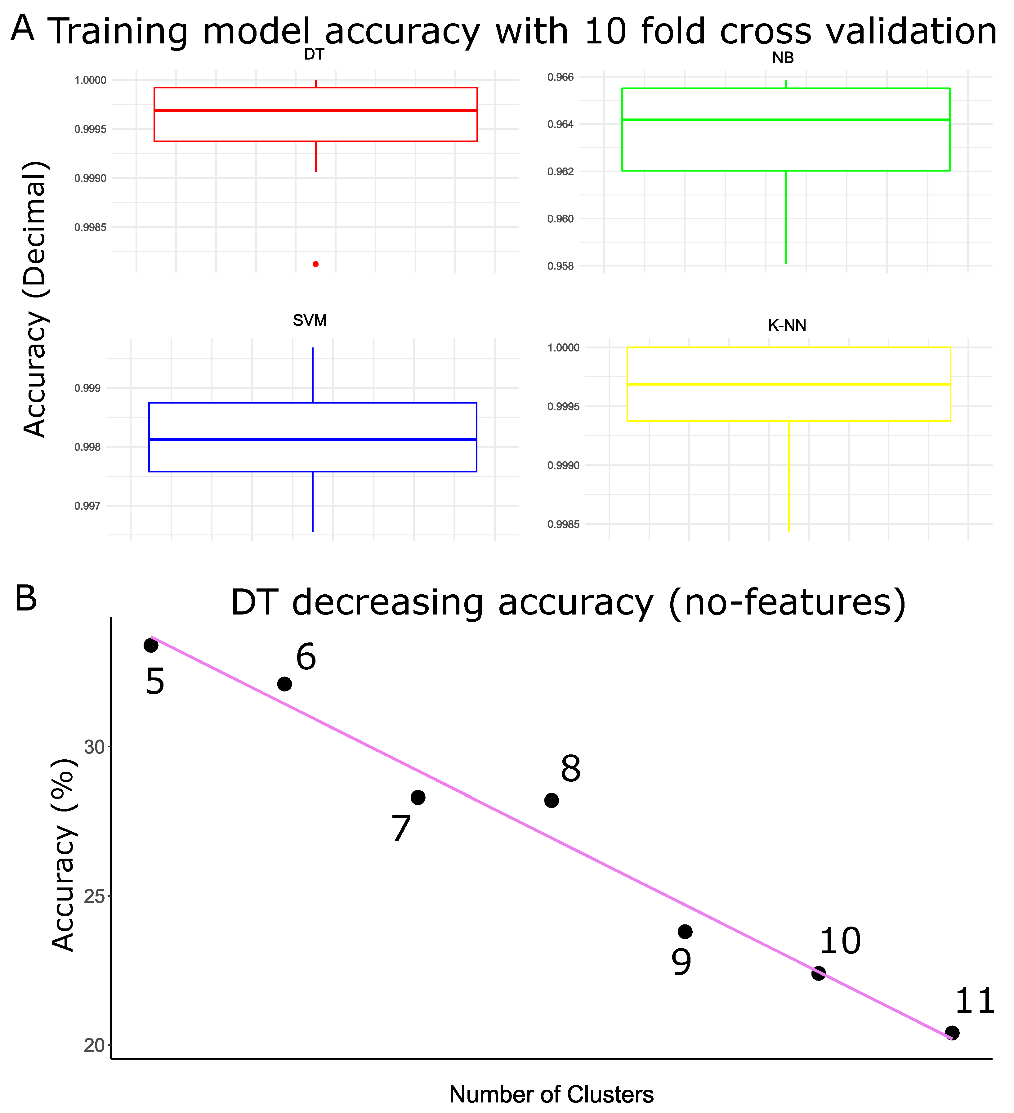
We trained different classifiers for the labeled data. The data were labeled based on the clusters. We performed 10-fold cross-validation procedure to validate our classification model (shown in Figure 5A). We further evaluated the model accuracy with the testing data. We found that our classification model could predict with an accuracy of 96.5–99.9%.

We also trained models without feature selection and extraction. We found that the accuracies of those models were consistent with most algorithms, except DT, as shown in

Table 2. Comparison of the accuracies of different methods evaluated using testing data.

Classifier		Clusters
		K = 5
	Accuracy%(Duration)		Accuracy% (Duration)
	Features sel.		No Features sel.
K-NN	99.9 (Low)		99.9 (Moderate)
NB	99.9 (Low)		99.3 (Low)
SVM	99.9 (Low)		99.7 (Very High)
DT	99.9 (Low)		58.0 (High)

Note: The categorical values were used to specify processing speeds rather than quantitative values (because quantitative values representing the processing speeds varied depending on the hardware (processor)). Moreover, the tuning parameters for classifiers were fixed while comparing feature selection and extraction against no-feature selection. This removes the analysis bias.

. DT accuracy was also sensitive to the number of classes when no features were selected or extracted, as shown in Figure 5B. The processing speed also slowed down for most algorithms due to the increased computation costs, as shown in Table 2.

However, the feature selection reduced the computation costs without loss of accuracy (robustness). In addition, we found that feature selection improves DT accuracy, as shown in Table 2. Therefore, our scheme provided low computation costs with feature selection and higher accuracy with different classifiers. Thus, our model can classify or detect different sub-phases during the IBM phase with high accuracy using different algorithms, and low computation costs, as shown in Table 2.

4. Discussion

We developed a pattern recognition and classification scheme to detect different sub-phases of IBMs during BH. We used force plates and estimated $\overrightarrow{a}$ and $\overrightarrow{j}$ to quantify the movements during contractions. Furthermore, we used phase portraits as a means to select features for our clustering and classification algorithms. We found that our designed scheme had a high processing speed, robustness, and accuracy using classifiers such as SVM, NB, DT, and K-NN. Our scheme will be of significant interest to practitioners working with the breathing disorder population. It can assist in detecting certain events of varying intensities within the IBM phase, thus diagnosing the extent of the breathing problem.

The use of kinetic, kinematics, and neural signals (EMG) is not uncommon for movement classification [16,17,18]. Based on the application of our study, the duration and strength of IBMs, kinetics, and kinematics are better choices for signal classification. A sensor review study validates it [19]. Moreover, sEMG-based classification was challenging because the muscles associated with IBMs are mostly deep (intercostal and diaphragm).

The circular geometry estimated from $\overrightarrow{a}$ and $\overrightarrow{j}$ phases during BH suggests rhythmic kinematic patterns of IBMs. Phase portrait-based comparative studies were performed on the locomotion of patients with Parkinson’s and without Parkinson’s that validate this hypothesis [20]. Although previous studies focused on movements where the joint angles during muscle contractions changed [21], our study is the first to use phase portraits for involuntary contraction analysis. Moreover, the variability in IBM amplitudes appeared as concentric circles in the phase portraits. Thus, the phase portraits provided good indicators of periodicity in signals with varying amplitudes. Moreover, phase portraits provided data about redundant features and crucial features. The redundant features were removed, whereas crucial features were extracted for cluster analysis. The processing, selection, and extraction of features using phase portrait increased the classification accuracy and reduced the computation burden.

4.1. Physiological Interpretation of Clusters

We used clusters to group different phases of the IBM phase. These groups displayed changes in $\overrightarrow{a}$ and $\overrightarrow{j}$ data values during a BH. We found from these clusters that there were sub-phases of low, moderate, and high magnitude within the IBM phase. The low values of $\overrightarrow{a}$ and $\overrightarrow{j}$ during IBMs were clustered with the NM phase in clusters 1 and 6. The low values of $\overrightarrow{a}$ and $\overrightarrow{j}$ in these clusters represented the onset of IBM. Moreover, the high and moderate data values of the IBM phase grouped in clusters 2, 3, 4, and 5 had physiological relevance to extend BH.

Our study showed that different levels of $\overrightarrow{a}$ and $\overrightarrow{j}$ clustered in groups 2, 3, 4, and 5 were correlated with force and associated with increasing IBM or the struggle phase during BH. The struggle phase is a phase in which participants can hold their breath beyond PB before reaching CB [10]. 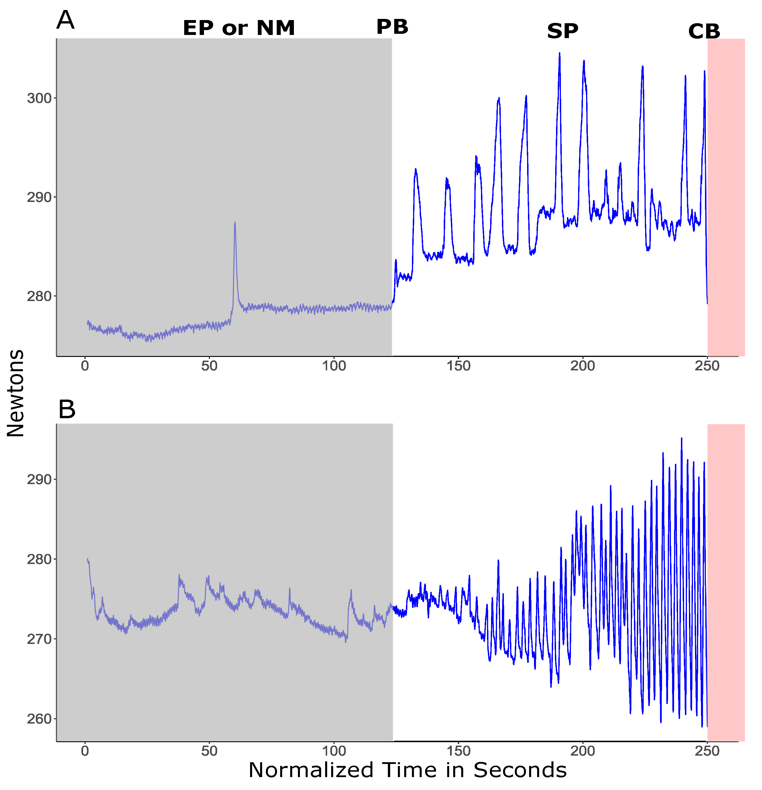A previous study showed that increased amplitude and the frequency of pressure signals are indicators of struggle termination [6,7,10]. In our study, we observed similar results for most participants, where force amplitude incremented continuously until the end of the SP, as shown in Figure 6B. However, in a few participants, the signal amplitude decayed before the SP ended, as shown in Figure 6A. The low force signal amplitude before the SP ended could have been due to a high fatigue index and low energy expenditure, as the $O_2$ level in blood during BH was depleting [22,23].

4.2. Accuracy, Speed, and Robustness

We used different classifiers that made no assumption about normality, such as SVM, DT, NB, and K-NN [24,25,26,27]. Our study also showed that the classification accuracy did not improve radically with feature selection and extraction as most classifiers performed well with the raw data. Moreover, accuracy did not decrease with an increase in the number of classes (clusters, K = 5 to 11). This creates a question about our scheme (pertaining to whether feature selection using phase portraits was necessary). The answer depends on the criteria considered for detection because we also found that the greedy algorithm, such as DT classification accuracy, was sensitive to feature selection, extraction, and the number of classes. Therefore, if the goal is to detect different IBM sub-phases with high accuracy and ignore other aspects, such as processing time and flexibility of using different algorithms, then feature selection and extraction using phase portraits are not necessary. However, ignoring these criteria will increase the hardware costs as faster processors and built-in computation methods will be needed. Therefore, our detection scheme offers high accuracy, speed, and flexibility with other algorithms without loss of accuracy (robustness).

The other aspect of the classification accuracy of our scheme is parameter optimization. We mentioned in our results that we kept parameters consistent while comparing the accuracy with and without feature selection. Hence, the DT model without features was not optimized subjectively to attain higher accuracy. The rationale was to reduce any analysis bias. However, the biased approach of optimizing the parameters for higher accuracy of the DT training model will not change the fact that there will still be a trade-off between accuracy and speed. Therefore, in our study, feature selection and extraction using phase portraits were of significant importance as they reduced the constraints related to the processing speed without impact accuracy [28], especially for greedy deterministic algorithms, such as DT.

4.3. Limitations and Future Work

There were information-based constraints with two-dimensional features ($\overrightarrow{a}$, $\overrightarrow{j}$) in this study. The lack of high-dimensional feature space limited the degree of freedom to process enough information. However, additional information could be captured using multichannel sensors with a high sampling rate. The inertial measurement unit (IMU) sensors could be alternates [19,29]. The IMUs were embedded with accelerators, gyroscopes, and magnetometers, and they could provide linear and rotational kinematic data about IBM in the vertical direction [29,30]. Therefore, a high-dimensional feature space can be acquired using such sensors and will be the scope of our future studies.

In addition, our study did not account for the relationships between physiological factors [31] (such as motivation level, blood lactic acid level, lung volume, partial levels of $O_2$ and $C{O}_2$ ($P{O}_2$ and $PC{O}_2$), and IBM sub-phases. Therefore, in this study, IBM’s physiological role was inferred. These physiological factors are the key factors for SP characteristic determination [7,10]. Thus, we could not develop a concrete relationship between IBM sub-phases and SP physiological characteristics. It is something we will consider studying in the future.

5. Conclusions

We found in our study that IBMs during BH could be captured through force sensors. In this study, we developed a pattern recognition and classification scheme using estimated $\overrightarrow{a}$ and $\overrightarrow{j}$ from the vertical ground reaction force. The $\overrightarrow{a}$ and $\overrightarrow{j}$ were used to quantify the rapid movements associated with involuntary contractions. Our scheme recognizes and classifies the IBM phase from the NM phase during BH, and also identifies and classifies different sub-phases of varying (low, moderate, and high) magnitudes within the IBM phase. We also developed phase portraits using $\overrightarrow{a}$ and $\overrightarrow{j}$ to select and extract specific features so that the accuracy, robustness, and computational costs of our scheme could be enhanced. To the best of our knowledge, this is the first study that developed a pattern recognition and classification scheme to detect IBMs from vertical ground reaction force.