A Bayesian Approach to Estimating Age from the Auricular Surface of the Ilium in Modern American Skeletal Samples

Abstract

Age estimation from human skeletal remains is a critical component of the biological profile for unidentified decedents. Using a Bayesian approach, we examine two popular methods (Lovejoy–LJ, and Buckberry zand Chamberlain–BC) for estimating age from the auricular surface of the ilium. Ages of transition are generated from a modern Portuguese skeletal sample (n = 466) and are coupled with an informative prior from historic Spitalfields, London (n = 179) to estimate age in a sample of modern Americans from the Bass Donated collection (n = 639). The Bass collection was challenging to statistically model, potentially due to higher morbidity and mortality characteristics of the central southern United States. The highest posterior density ranges provide a realized accuracy between 84–89% for males and 85–91% for females using the LJ method, and a realized accuracy between 79–82% for males and 65–71% for females using the BC method. Both methods worked well for older individuals. Cumulative binomials showed that both methods significantly underperformed; however, results were better for the LJ method, which also showed lower bias. Reference tables for aging modern American samples are provided, and the data meet Daubert guidelines, i.e., legal criteria for acceptable scientific evidence in a court of law in the United States.

1. Introduction

An important component in building the biological profile for an unidentified decedent is the estimation of age-at-death. Adult age estimation is particularly challenging because it is based on the degeneration of the skeletal tissue, which is further affected by an individual’s life history. These biological and environmental processes result in considerable variation in age indicators, especially for middle to older adults.

Traditionally, skeletal age is estimated by scoring features on a reference sample where morphological changes in the skeleton are linked with known age and then applying these estimated ages to an unknown target sample or individual. In a severe critique, Bocquet-Appel and Masset [1] outlined the bias and inaccuracy inherent in this approach, where the age distribution of the target sample will reflect the age distribution of the reference sample, a condition which later came to be known as age mimicry. Boldsen and colleagues [2] proposed transition analysis, a method that reduces or eliminates the issue of age mimicry. When transition analysis parameters are combined with Bayesian statistics using a prior age distribution, the resulting age estimates more accurately reflect the senescence changes in the target sample while minimizing bias [2]. Bayesian statistics with transition analysis have been successfully applied to pelvic age indicators, including the pubic symphysis [3,4,5,6] and the auricular surface [7,8,9].

Lovejoy and colleagues [10] developed the traditional, standardized method for estimating age-at-death based on morphological changes to the auricular surface of the ilium. Their method (referred to here as the Lovejoy method, LJ), based on an eight-phase system, describes changes to several criteria (e.g., transverse organization, texture, porosity, etc.) and is considered advantageous because the changes manifest well into advanced years. While widely used across various geographic regions, most authors reported broad agreement when applying the Lovejoy method [11,12,13,14,15,16,17,18,19]. However, as one might expect, this traditional approach suffered from typical issues of age mimicry and some researchers struggled to assign a myriad of morphological changes to one stage. This latter issue was specifically addressed by Lovejoy and colleagues, who proposed that scholars should focus on the critical age indicators that best represent the aging process and use auxiliary features to adjust age estimates.

Buckberry and Chamberlain [20] used a different approach to revise the auricular surface aging method (referred to here as Buckberry and Chamberlain method, BC). They argued that the auricular surface features aged independently from one another and should be scored separately and not grouped together into a single phase. Thus, instead of combining various indicators into a single phase, they created a composite scoring system where five features (transverse organization, texture, microporosity, macroporosity, and apical changes) were independently scored and then combined to estimate a final composite age for the individual. They reported increased replicability, due in part to lower intra- and inter-observer error. Importantly, while results were presented using a traditional statistical approach, the authors also used Bayesian statistics to provide posterior probabilities for ten-year age ranges. Some authors [21,22] compared the LJ and BC methods and found BC markedly easier to apply and more accurate than the LJ method. In 2016, Hens and Godde [7] applied Bayesian methodology to both auricular surface methods, statistically modeling age in Portuguese males. They found that the application of transition analysis coupled with Bayesian statistics significantly improved age estimates for both methods, work that was later independently confirmed by Kim and Algee-Hewitt [23].

The main objective of this research is to use a Bayesian analysis to apply an informative prior probability distribution with transition analysis to estimate age-at-death in a modern American skeletal sample of both males and females. We compare the Lovejoy and Buckberry and Chamberlain methods. The resulting age estimates are tested for performance against a hold-out sample of Americans, an issue considered critical by Braga et al. [24]. This Bayesian approach allows for the estimation of accuracy and precision (i.e., bias) for each method. Our second objective is to provide the highest posterior density ages and highest posterior density age ranges at 75%, 90%, and 95% accuracy (i.e., coverages) that may be used by forensic anthropologists practicing in a legal setting who need to estimate the age of unknown individuals. These results meet the criteria outlined in Daubert v. Merrell Dow Pharmaceuticals, Inc. [25] which required rigorous testing and evaluation of forensic methods. Referred to as the Daubert guidelines, this case law outlines the criteria needed for the presentation of scientific evidence in a court of law. Specifically, the United States Supreme Court determined that in order for evidence to be considered reliable, it must be grounded in scientific methods and procedures, i.e., the technique has been subjected to peer review, error rates are reported, and the technique is generally accepted within the relevant scientific community. The 75% coverage would be acceptable for skeletal remains in archaeological contexts, where personal identification of decedents is highly unlikely or impossible and age estimation is provided as a foundation for further demographic or pathological interpretations. However, the 90% and 95% coverages meet the standards outlined for reliability in the Daubert guidelines where accuracy and precision in age estimates are essential.

2. Materials and Methods

2.1. Samples and Scoring

This research uses two contemporary, modern skeletal samples: (1) American males and females of European (i.e., White) ancestry derived from the William M. Bass Donated Skeletal Collection at the University of Tennessee Knoxville (Bass Collection) and (2) Portuguese males and females from the Luis Lopes Collection of the National Museum of Natural History and Science in Lisbon, Portugal (Lopes Collection). Both collections are associated with documented demographic characteristics. Background on collection history and composition are presented by Shirley et al. [26] and Cardoso [27], and the samples have been thoroughly described in the literature [3,4,7,8,28]. A third sample from Christ Church Spitalfields (Natural History Museum, London) dates to post-medieval London residents and is dated to 1646–1859 AD. This sample also has documented age, sex, and occupation for a portion of the collection [29] and served as the sample for Buckberry and Chamberlain’s [20] work. The Spitalfields sample has a similar age profile to our two modern samples.

Table 1. Sample age distributions.

Age Interval	American	Portuguese	Spitalfields
	Males/Females	Males/Females	Males/Females
16–19	1/0	5/5	2/2
20–29	7/3	18/22	5/5
30–39	44/12	20/10	14/9
40–49	72/30	34/12	8/11
50–59	83/57	49/39	15/22
60–69	80/67	35/43	25/19
70–79	50/60	33/66	13/16
80–89	35/38	27/43	2/9
90–99	0/0	0/5	2/0
Total	372/267	221/245	86/93

depicts a breakdown of the samples by sex and age for each collection.

The American and Portuguese samples were scored by one experienced researcher (SMH) for the two auricular surface methods, LJ and BC, using protocols to maintain a blind study. Pathological specimens and individuals of unknown sex were not scored. All Portuguese pelves were scored across a period of two weeks, while the Americans were scored during one week. To account for intraobserver error, ten pelves from each collection were scored three times each on different days and there was perfect agreement. Additionally, due to the challenging nature of the LJ method, wherein one must combine numerous indicators into one stage, scoring followed guidelines outlined by Lovejoy et al. [10] where individuals exhibiting traits indicative of an advanced stage were placed into a higher phase/stage even when youthful characteristics were retained. We lament cases where authors have not reported their scoring techniques thoroughly in the literature.

2.2. Statistical Methodology

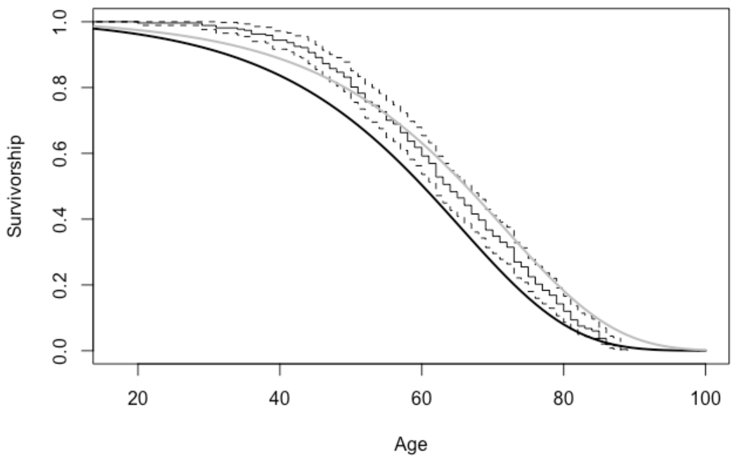
For the goal of this paper, the American data (Bass collection) serve as the target sample to derive and test age-at-death estimates from the two auricular surface aging methods. The Portuguese data (Lopes collection) are used to estimate the transition analysis (TA) parameters. The Spitalfields sample serves as the informative prior, from which we calculated hazard parameters using a Gompertz model. These Gompertz parameters are subsequently combined with the Portugal TA parameters in Bayes Theorem to produce point estimates and ranges of ages to be tested on the American sample. Plots of Kaplan–Meier survivorship calculated on American females and males with Gompertz curves from the Portuguese and Spitalfields data confirm the fit of these samples (Figure 1 and Figure 2). Selection of similar mortuary profiles generally ensures a good fit of the informative prior to the age-at-death structure in the TA sample [6]. However, Godde and Hens [3] reported some deviation from fit may be tolerated; a conclusion that was later confirmed by the independent work of other researchers [9,30].

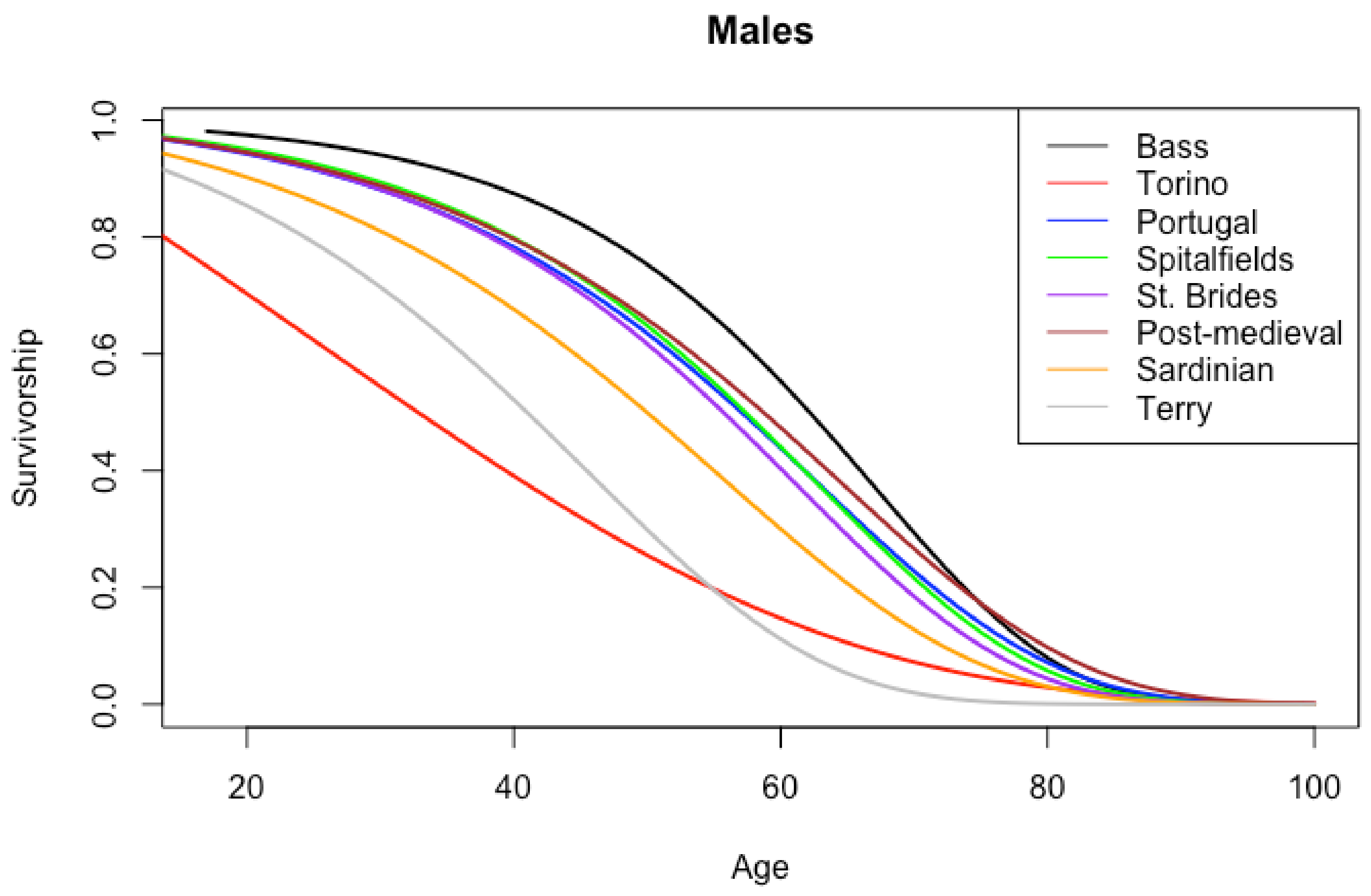
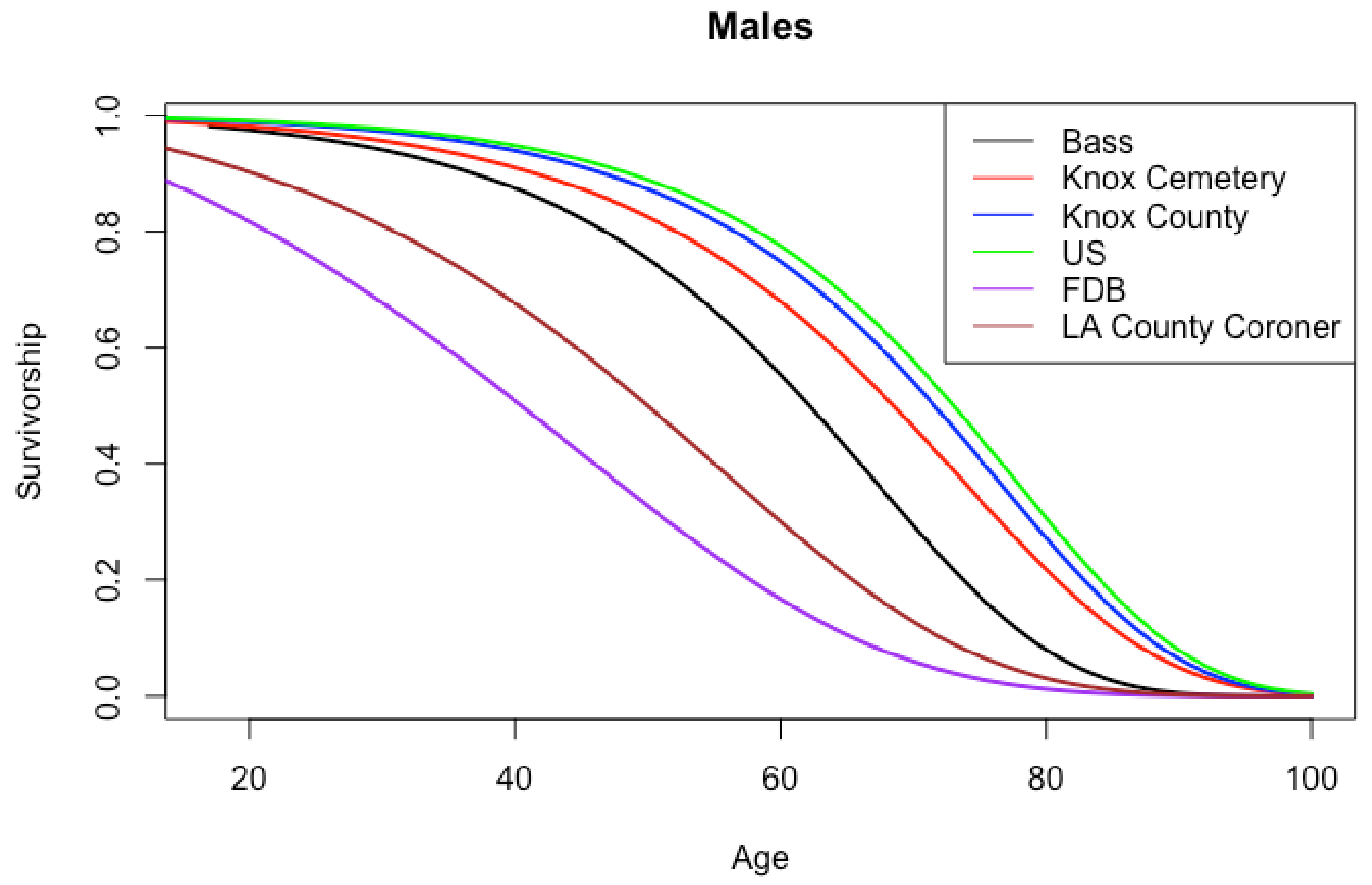
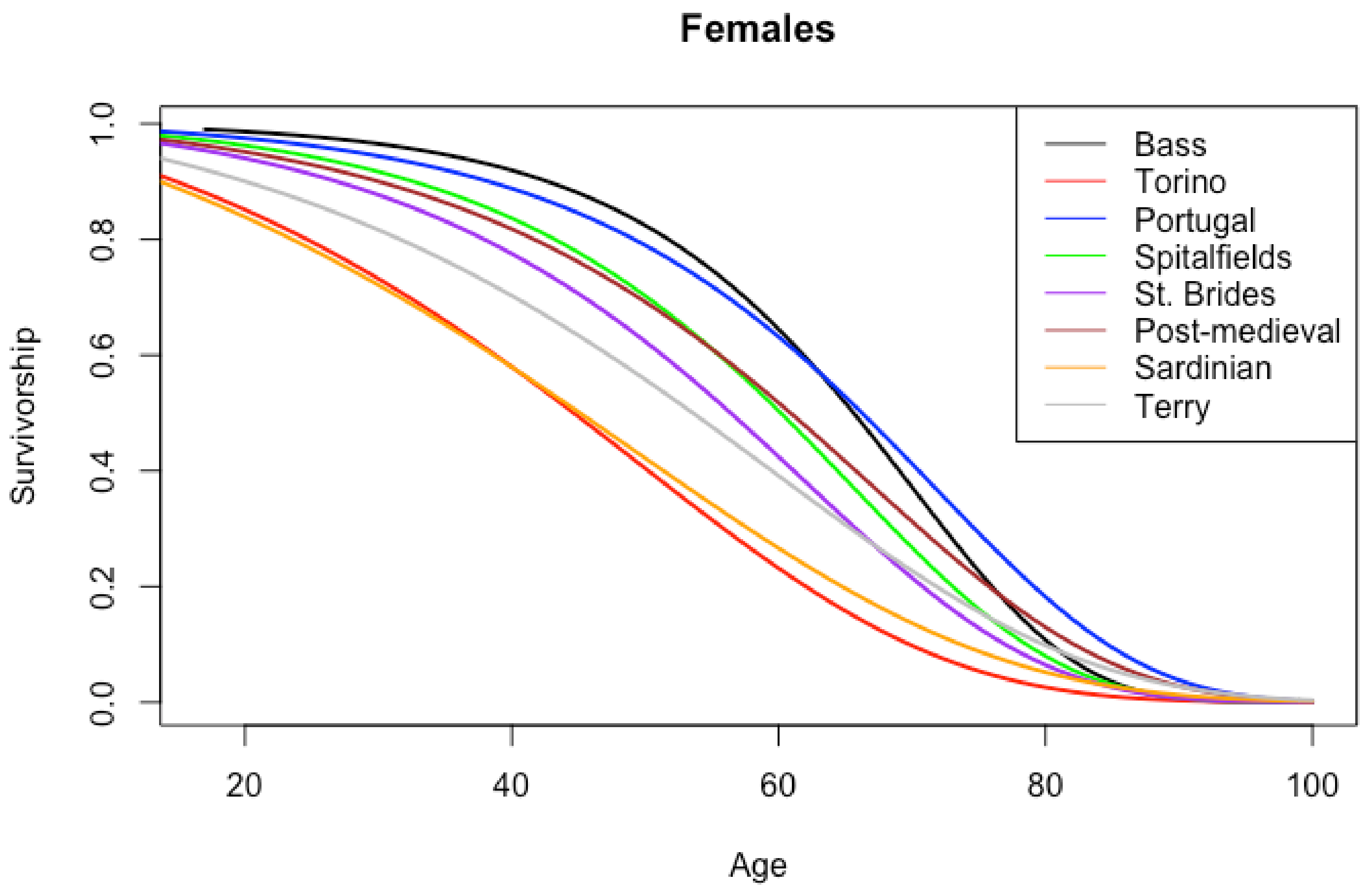
A number of samples were available from which to choose an informative prior, either through published Gompertz parameters (Terry collection, LA County Coroner from Konigsberg et al. [6]), Knox County, Knox Cemetery, U.S. from census data in Godde [8], or the generation of Gompertz parameters from our own data with published Gompertz parameters (Torino, Portugal, Sardinia) [3,4,7,31], unpublished data of which we were granted access (Forensic Databank, St. Brides [32]), publicly available data (post-medieval England and Wales as described in Godde and Hens [3,4,7,33]), and the data published in Buckberry and Chamberlain [20]. Past attempts at modeling the American sample showed the available samples (except those from post-medieval Europe) were not a good fit and did not produce viable age ranges. Gompertz survivorship plots of the three European samples (Figure 3, Figure 4 and Figure 5) showed St. Brides and Spitalfields had promise as their fit to the Bass Collection was good, as was their relationship to the sample from Portugal. The decision to go with Spitalfields over St. Brides was driven by a slightly better fit of TA parameters.

The Gompertz model is expressed as:

$$h_t={\alpha }_3{e}^{{\beta }_{3}t}$$

(1)

$$S\left(t\right)=\exp \left\{\frac{{\alpha }_3}{{\beta }_3}\left[1-\exp \left({\beta }_{3}t\right)\right]\right\}$$

(2)

where h is the hazard, t is age-at-death, and S is survivorship; Equation (1) is the hazard and Equation (2) is the survival function. The Gompertz model parameters are α₃ and β₃. We did not shift our curve to a specific age. The transition analysis parameters were obtained from a cumulative probit model [6], which represent the age at which an individual transitions from, in this case, one auricular surface phase to the next. The probits were run for: (1) Lovejoy method phases, (2) each of the five indicators for Buckberry and Chamberlain, and (3) the composite scores as phases from Buckberry and Chamberlain. The transition analysis and Gompertz model parameters are combined in Bayes’ theorem [2]:

$$\mathrm{Pr}\left(a|c_j\right)=\frac{\mathrm{Pr} \left(c_j|a\right)f\left(a\right)}{{{\displaystyle \int }}_0^{\infty }\mathrm{Pr}\left(c_j|x\right)f\left(x\right)dx }$$

(3)

where f(a) is a probability density function (PDF) used to derive the highest posterior density (HPD), analogous to a frequentist mode, and highest posterior density region (HPDR), which is a range of values calculated at 75%, 90%, and 95% coverages. Coverage represents the “percentage of individuals expected to fall within the specified HPDR” [6]. Due to this property, as the coverages increase, the regions become larger. In this paper, we use the HPDRs as age ranges.

The accuracy of the HPDRs was tested by a cumulative binomial test using the documented age of the American samples as a measure of the accuracy of the HPDRs at the various coverages. A measure of accuracy and whether it is significantly different than the stated coverage is provided through this process. Finally, bias is estimated and reported with the following equation:

$$\mathsf{\Sigma } \frac{\left(estimated age-actual age\right)}{N}$$

(4)

All analyses were run in R [34] using originally composed scripts and programming written by Dr. Lyle Konigsberg (http://faculty.las.illinois.edu/lylek/, accessed on 25 June 2022).

3. Results

TA parameters for Lovejoy method phases in females and males are found in

Table 2. Transition analysis parameters for Lovejoy et al. method on Portuguese samples.

Parameter	Estimate	Age at Transition	Estimate	Age at Transition
	MALES		FEMALES
I-II	2.97	19.45	3.05	21.17
II-III	3.28	26.47	3.37	29.16
III-IV	3.55	34.89	3.62	37.38
IV-V	3.81	45.18	3.86	47.29
V-VI	4.08	59.28	4.03	56.45
VI-VII	4.29	72.91	4.16	63.87
VII-VIII	4.53	92.75	4.40	81.80
ST DEV	0.25		0.23
b	4.04		4.28
Log-likelihood	−303.65		−324.73

. Female ages-at-transition are spread almost across each decade of life until phases 7–8 at which point it jumps to 2 decades. In males, each age-at-transition until phases 6–7 represents a single decade of life. At phases 6–7, this changes to every 2 decades, similar to the females. The Buckberry and Chamberlain method TA parameters in

Table 3. Transition analysis parameters for transverse organization using Buckberry and Chamberlain method on Portuguese samples. Estimates and slope are on a log scale.

Parameter	Estimate	Age at Transition	Estimate	Age at Transition
	MALES		FEMALES
I-II	3.04	20.96	3.14	23.26
II-III	3.55	34.86	3.61	36.95
III-IV	3.86	47.31	3.91	49.82
IV-V	4.40	81.63	4.43	83.92
ST DEV	0.40		0.43
b	2.52		2.30
Log-likelihood	−258.58		−293.02

,

Table 4. Transition analysis parameters for texture using Buckberry and Chamberlain method on Portuguese samples. Estimates and slope are on a log scale.

Parameter	Estimate	Age at Transition	Estimate	Age at Transition
	MALES		FEMALES
I-II	2.93	18.69	3.04	20.84
II-III	3.29	26.94	3.51	33.42
III-IV	3.75	42.55	3.83	45.98
IV-V	4.00	54.36	4.01	55.08
ST DEV	0.32		0.29
b	3.12		3.50
Log-likelihood	−205.14		−181.16

,

Table 5. Transition analysis parameters for apical changes using Buckberry and Chamberlain method on Portuguese samples. Estimates and slope are on a log scale.

Parameter	Estimate	Age at Transition	Estimate	Age at Transition
	MALES		FEMALES
I-II	3.47	32.14	3.55	34.81
II-III	4.32	75.47	4.21	67.04
ST DEV	0.52		0.47
b	1.92		2.11
Log-likelihood	−192.38		−204.25

,

Table 6. Transition analysis parameters for microporosity using Buckberry and Chamberlain method on Portuguese samples. Estimates and slope are on a log scale.

Parameter	Estimate	Age at Transition	Estimate	Age at Transition
	MALES		FEMALES
I-II	3.46	31.73	3.33	27.89
II-III	3.78	43.71	3.63	37.82
ST DEV	0.53		0.47
b	1.89		2.14
Log-likelihood	−167.89		−119.71

,

Table 7. Transition analysis parameters for macroporosity using Buckberry and Chamberlain method on Portuguese samples. Estimates and slope are on a log scale.

Parameter	Estimate	Age at Transition	Estimate	Age at Transition
	MALES		FEMALES
I-II	3.63	37.76	3.54	34.53
II-III	4.58	97.24	4.22	68.01
ST DEV	0.74		0.49
b	1.35		2.04
Log-likelihood	−214.93		−207.04

and

Table 8. Transition analysis parameters for Buckberry and Chamberlain Phases on Portuguese samples. Estimates and slope are on a log scale.

Parameter	Estimate	Age at Transition	Estimate	Age at Transition
	MALES		FEMALES
I-II	2.96	19.25	3.04	20.96
II-III	3.25	25.84	3.38	29.48
III-IV	3.50	32.98	3.55	34.92
IV-V	3.77	43.54	3.73	41.74
V-VI	4.00	54.73	3.94	51.48
VI-VII	4.26	71.03	4.20	66.90
ST DEV	0.30		0.30
b	3.30		3.29
Log-likelihood	−293.97		−278.58

have relatively similar patterns across the sexes and show several components that distinguish between young and older adults (i.e., apex and macroporosity). Microporosity does not distinguish between major life stages (e.g., young, middle, and older adult), concentrating on discriminating with an approximately 10–12 year age range in both sexes. Texture ages-at-transition are spread from young–middle adult among the sexes, while transverse organization is spread from young–middle until stages 4–5 at which time it increases to the 80s. Finally, for both sexes the phases derived from composite scores extend relatively evenly until older adult.

The HPDR table for the LJ method phases shows similar ranges for females and males (

Table 9. Highest posterior density (HPD) for each Lovejoy method phase with various highest posterior density regions (HPDR) in the American samples using Spitalfields samples as the informative prior.

Phase	HPD	75% HPDR	90% HPDR	95% HPDR
MALES
		63.44% Realized Accuracy	83.87% Realized Accuracy	88.98% Realized Accuracy
I	18.00	18.00–25.24	18.00–29.15	18.00–31.91
II	25.18	18.71–33.95	18.00–39.25	18.00–43.31
III	34.85	25.2–48.2	22.01–55.12	20.26–59.78
IV	47.04	34.45–63.50	30.20–71.39	27.79–76.45
V	61.79	46.74–78.51	41.19–85.46	37.96–89.66
VI	73.28	57.96–88.06	51.75–93.81	48.01–97.23
VII	81.36	66.74–94.44	60.41–99.39	56.47–102.34
VIII	89.14	75.72–100.64	69.60–104.95	65.68–107.50
FEMALES
		65.17% Realized Accuracy	85.39% Realized Accuracy	91.39% Realized Accuracy
I	18.00	18.00–26.07	18.00–30.15	18.00–32.99
II	27.77	20.53–37.61	18.26–42.33	18.00–46.27
III	37.94	27.96–51.49	24.58–58.49	22.68–63.27
IV	49.78	37.14–66.03	32.80–73.73	30.32–78.67
V	61.38	47.06–77.78	41.83–84.77	38.78–89.04
VI	69.65	54.76–85.02	48.98–91.18	45.53–94.88
VII	78.55	63.52–92.41	57.21–97.68	53.35–100.81
VIII	89.10	75.15–100.91	68.80–105.26	64.76–107.83

). The regions increase with phases, which is expected due to increased heterogeneity as one ages. In comparison with the HPDRs generated from the BC method (

Table 10. Highest posterior density (HPD) for each Buckberry and Chamberlain phase with various highest posterior density regions (HPDR) in the American samples using Spitalfields samples as the informative prior.

Phase	HPD	75% HPDR	90% HPDR	95% HPDR
MALES
		62.10% Realized Accuracy	79.03% Realized Accuracy	82.26% Realized Accuracy
I	18.00	18.0–27.9	18.00–33.52	18.00–37.62
II	26.01	18.04–37.69	18.00–45.99	18.00–51.78
III	35.63	24.04–52.85	20.56–61.58	18.75–67.09
IV	48.89	33.73–68.74	28.79–77.53	26.05–82.83
V	62.67	45.38–80.84	38.99–87.96	35.30–92.15
VI	73.36	55.94–89.12	48.76–94.96	44.46–98.39
VII	85.00	68.86–98.19	61.43–102.93	56.73–105.69
FEMALES
		50.56% Realized Accuracy	64.79% Realized Accuracy	71.16% Realized Accuracy
I	18.00	18.00–29.89	18.00–36.4	18.00–41.12
II	30.17	20.19–45.36	18.00–53.57	18.00–60.24
III	40.48	27.42–59.57	23.43–69.00	21.29–74.91
IV	50.11	34.67–70.38	29.65–79.29	26.85–84.62
V	61.88	44.29–80.81	37.92–88.22	34.27–92.54
VI	73.38	55.31–89.61	47.93–95.55	43.54–99.01
VII	86.43	69.86–99.59	62.13–104.23	57.21–106.92

), the Lovejoy method’s regions were narrower by phase. Both aging techniques detected older ages.

The cumulative binomials (

Table 11. Cumulative binomial tests of the performance of the Lovejoy (LJ) and Buckberry and Chamberlain (BC) methods on American holdout samples using Portuguese transition analysis parameters and Spitalfields samples as the informative prior.

Method	CI	Number of Successes	Number of Failures	p-Value	Probability of Success	Bias
MALES
LJ	75%	236	136	<0.0001	0.63	7.95
LJ	90%	312	60	0.0003	0.84	8.33
LJ	95%	331	41	<0.0001	0.89	8.62
BC	75%	231	141	<0.0001	0.62	10.85
BC	90%	294	78	<0.0001	0.79	10.77
BC	95%	306	66	<0.0001	0.82	11.49
FEMALES
LJ	75%	174	93	0.0004	0.65	7.99
LJ	90%	228	39	0.0183	0.85	8.04
LJ	95%	244	23	0.0109	0.91	8.09
BC	75%	135	132	<0.0001	0.51	−10.91
BC	90%	173	94	<0.0001	0.65	−11.02
BC	95%	190	77	<0.0001	0.71	−11.08

Bold indicates significantly lower performance than probability.

) show that neither method’s accuracy met the corresponding coverage level; they all significantly underperformed. However, the realized accuracies for the Lovejoy method coverages were still good–excellent, especially for the 90% coverage, yielding approximately 91% accuracy in females and 89% accuracy in males. Biases indicate that the LJ technique overaged for both sexes, while the BC method underaged females and overaged males. In general, the bias was greater for the BC method. Taken together, the results from the LJ method technique were superior to BC—at least for the American target sample.

4. Discussion

Age estimation from the auricular surface of the ilium remains a popular method utilized by forensic anthropologists, with the LJ method garnering more than twice as many practitioners as the BC method in a recent survey [35]. The BC method is reportedly easier to apply and outperforms the LJ method when no statistical manipulations are applied [7,21,22]. The BC method should be the technique of choice when practitioners are unable to use Bayesian statistics. However, previous work on Portuguese males [7] strongly indicated that while both methods perform relatively equally when Bayesian statistics are applied, the LJ method showed significant improvement under this rigorous methodology compared with a traditional (i.e., non-Bayesian) approach. There is little reason for forensic anthropologists to apply the traditional LJ method without the use of a Bayesian approach. Additionally, the auricular surface of the ilium outperforms the commonly used Suchey–Brooks pubic symphysis method, providing narrower age ranges with better coverages (see ranges in Godde and Hens [3,4] for comparison).

This paper used Bayesian modeling to estimate age in modern Americans from both sexes and supports our previous work modeling age in Portuguese males [7]. When contrasting these two aging methods on Americans of both sexes, the LJ method showed narrower age ranges and lower bias, around 8%, compared with around 11% using BC. Additionally, the LJ method showed higher realized accuracy at 75%, 90%, and 95% coverages, and markedly so for females, where accuracy was between 15–20% higher using LJ. The HPDRs reported here control for age mimicry, allowing age estimates to be applied across different populations. Forensic anthropologists should feel comfortable using the HPDR tables presented here, along with our previously published values for Portuguese males [7] as look-up tables for their own data and avoiding non-Bayesian auricular surface aging, especially for the LJ method. Indeed, Konigsberg et al. [6] argue that population-specific age indicators are not as important as comparable age structures between populations.

Admittedly, we attempted to model age in the American sample previously but were unable to find a comparable sample with a good fit to use as an informative prior. The Bass Donated collection represents a sample of modern Americans drawn primarily from Tennessee, but also other regions in the central south of the United States; one would think comparable populations would abound. In a 2017 paper, Godde [8] noted the Bass Collection Gompertz survivorship was significantly different than a cemetery from the same city and the mortality data from the U.S. Census for the same county, state, and country (also visible in Figure 3, Figure 4 and Figure 5). Thus, we were challenged in finding a sample with a similar age distribution until we accessed the data from Spitalfields and St. Brides. When choosing a prior, it is customary to search for populations that are comparable in terms of time and geography. Why would a sample of post-medieval Londoners have provided such a good fit to modern Americans from the south? In particular, for females, the lower survivorship of around age 83 and over almost mirrors post-medieval Europe. Additionally, the roughly contemporary Portuguese sample, representing urban as well as rural-to-urban migrants, also matched with the modern Americans. An exploration of the literature on health and mortality provides some insights as to why it was so tough to fit a model to the Bass collection.

In general, mortality in the United States is higher than in countries with similar economies [36]. While health and mortality may vary due to numerous factors including socioeconomic status, sex, and ethnicity, geography remains a significant factor. Geographic inequality in adult mortality in the United States is greater than in western Europe [37] and the central-southern section of the United States is one of the most disadvantaged [38], especially since the mid-20th century [39].

The rural southern United States, especially Tennessee, Kentucky, Alabama, and Mississippi, has higher rates of morbidity and mortality compared with other rural and urban areas in the Northeast, Midwest, and Western United States [40,41]. In particular, Appalachia and the Mississippi Delta regions have the lowest life expectancy in the country and the highest mortality rates due to various health issues [42,43,44,45,46]. People from Tennessee and Appalachia are the main contributors to the Bass Donated collection [26].

Mortality rates in the last two decades in many southern states (including Tennessee) were 30–40% higher than other regions of the United States—translating to 3–4 fewer years of life expected at age 50 [36]. These values represent the effects of numerous environmental and health hazards, including: smoking [36]; lower bone mineral density with higher hip fracture rates [47]; nutritional disease [48]; growth stunting [49]; stroke [50,51]; and high helminth load, with up to 55% of people affected by endemic whipworm, despite campaigns to eradicate such infections [52]. Overall, these studies underscore the poorer health and increased mortality risk from structural inequalities in populations from the central south United States, which is the underlying population for the Bass Donated collection. The health and mortality of these U.S. southerners more closely matches that from post-medieval London and urbanizing Lisbon in the 1800s who would have been affected with similar environments [28].

Despite the challenges inherent in modeling the Americans, we are successful in providing highest posterior density ages and highest posterior age ranges for modern American samples. Tests on a hold-out sample show realized accuracy in the 80–90% range. The Bayesian approach is far superior to traditional (i.e., non-Bayesian) methods because it controls for age mimicry, allowing age estimates to be applied across different populations. Additionally, Bayesian methods provide prediction intervals and/or credible intervals. Some forensic anthropologists may find the wide age ranges disappointing and hesitate to apply them to their own casework. We would remind them that these estimates are far superior to the traditional auricular surface age estimates alone and these statistical approaches are necessary to meet Daubert criteria in American forensic science.

References

1. Bocquet-Appel, J.-P.; Masset, C. Farewell to Paleodemography. J. Hum. Evol. 1982, 11, 321–333. [Google Scholar] [CrossRef]
2. Boldsen, J.; Milner, G.; Konigsberg, L.; Wood, J. Transition Analysis: A New Method for Estimating Age from Skeletons. In Paleodemography: Age Distributions from Skeletal Samples; Hoppa, R.D., Vaupel, J.W., Eds.; Cambridge University Press: Cambridge, UK, 2002; pp. 73–108. [Google Scholar]
3. Godde, K.; Hens, S.M. Age-at-Death Estimation in an Italian Historical Sample: A Test of the Suchey-Brooks and Transition Analysis Methods. Am. J. Phys. Anthropol. 2012, 149, 259–265. [Google Scholar] [CrossRef] [PubMed]
4. Godde, K.; Hens, S.M. Modeling Senescence Changes of the Pubic Symphysis in Historic Italian Populations: A Comparison of the Rostock and Forensic Approaches to Aging Using Transition Analysis. Am. J. Phys. Anthropol. 2015, 156, 466–473. [Google Scholar] [CrossRef] [PubMed]
5. Kimmerle, E.H.; Konigsberg, L.W.; Jantz, R.L.; Baraybar, J.P. Analysis of Age-at-Death Estimation through the Use of Pubic Symphyseal Data. J. Forensic Sci. 2008, 53, 558–568. [Google Scholar] [CrossRef] [PubMed]
6. Konigsberg, L.W.; Herrmann, N.P.; Wescott, D.J.; Kimmerle, E.H. Estimation and Evidence in Forensic Anthropology: Age-at-Death. J. Forensic Sci. 2008, 53, 541–557. [Google Scholar] [CrossRef] [PubMed]
7. Hens, S.M.; Godde, K. Auricular Surface Aging: Comparing Two Methods That Assess Morphological Change in the Ilium with Bayesian Analyses. J. Forensic Sci. 2016, 61 (Suppl. S1), S30–S38. [Google Scholar] [CrossRef]
8. Godde, K. The Use of Informative Priors in Bayesian Modeling Age-at-Death; a Quick Look at Chronological and Biological Age Changes in the Sacroiliac Joint in American Males. AIMS Public Health 2017, 4, 278. [Google Scholar] [CrossRef]
9. Nikita, E.; Xanthopoulou, P.; Kranioti, E. An Evaluation of Bayesian Age Estimation Using the Auricular Surface in Modern Greek Material. Forensic Sci. Int. 2018, 291, 1–11. [Google Scholar] [CrossRef] [Green Version]
10. Lovejoy, C.; Meindl, R.; Pryzbeck, T. Chronological Metamorphosis of the Auricular Surface of the Ilium: A New Method for the Determination of Adult Skeletal Age at Death. Am. J. Phys. Anthropol. 1985, 68, 15–28. [Google Scholar] [CrossRef]
11. Murray, K.; Murray, T. A Test of the Auricular Surface Aging Techniques. J. Forensic Sci. 1991, 36, 1163–1169. [Google Scholar] [CrossRef]
12. Martrille, L.; Ubelaker, D.H.; Cattaneo, C.; Seguret, F.; Tremblay, M.; Baccino, E. Comparison of Four Skeletal Methods for the Estimation of Age at Death on White and Black Adults. J. Forensic Sci. 2007, 52, 302–307. [Google Scholar] [CrossRef]
13. Saunders, S.R.; Fitzgerald, C.; Rogers, T.; Dudar, C.; McKillop, H. A Test of Several Methods of Skeletal Age Estimation Using a Documented Archaeological Sample. Can. Soc. Forensic Sci. J. 1992, 25, 97–118. [Google Scholar] [CrossRef]
14. Bedford, M.E.; Russell, K.F.; Lovejoy, C.O.; Meindl, R.S.; Simpson, S.W.; Stuart-Macadam, P.L. Test of the multifactorial aging method using skeletons with known ages-at-death from the grant collection. Am. J. Phys. Anthropol. 1993, 91, 287–297. [Google Scholar] [CrossRef]
15. Falys, C.G.; Schutkowski, H.; Weston, D.A. Auricular Surface Aging: Worse than Expected? A Test of the Revised Method on a Documented Historic Skeletal Assemblage. Am. J. Phys. Anthropol. 2006, 130, 508–513. [Google Scholar] [CrossRef]
16. Storey, R. An elusive paleodemography? A comparison of two methods for estimating the adult age distribution of deaths at late Classic Copan, Honduras. Am. J. Phys. Anthropol. 2007, 132, 40–47. [Google Scholar] [CrossRef]
17. Rougé-Maillart, C.; Vielle, B.; Jousset, N.; Chappard, D.; Telmon, N.; Cunha, E. Development of a Method to Estimate Skeletal Age at Death in Adults Using the Acetabulum and the Auricular Surface on a Portuguese Population. Forensic Sci. Int. 2009, 188, 91–95. [Google Scholar] [CrossRef] [Green Version]
18. Schmitt, A. Age-at-Death Assessment Using the Os Pubis and the Auricular Surface of the Ilium: A Test on an Identified Asian Sample. Int. J. Osteoarchaeol. 2004, 14, 1–6. [Google Scholar] [CrossRef]
19. Hens, S.M.; Rastelli, E.; Belcastro, G. Age Estimation from the Human Os Coxa: A Test on a Documented Italian Collection. J. Forensic Sci. 2008, 53, 1040–1043. [Google Scholar] [CrossRef]
20. Buckberry, J.L.; Chamberlain, A.T. Age Estimation from the Auricular Surface of the Ilium: A Revised Method. Am. J. Phys. Anthropol. 2002, 119, 231–239. [Google Scholar] [CrossRef]
21. Hens, S.M.; Belcastro, M.G. Auricular Surface Aging: A Blind Test of the Revised Method on Historic Italians from Sardinia. Forensic Sci. Int. 2012, 214, 209.e1–209.e5. [Google Scholar] [CrossRef]
22. Mulhern, D.M.; Jones, E.B. Test of revised method of age estimation from the auricular surface of the ilium. Am. J. Phys. Anthropol. 2005, 126, 61–65. [Google Scholar] [CrossRef] [PubMed]
23. Kim, J.; Algee-Hewitt, B.F.B. Age-at-Death Patterns and Transition Analysis Trends for Three Asian Populations: Implications for [Paleo]Demography. Am. J. Biol. Anthropol. 2022, 177, 207–222. [Google Scholar] [CrossRef]
24. Braga, J.; Heuze, Y.; Chabadel, O.; Sonan, N.K.; Gueramy, A. Non-Adult Dental Age Assessment: Correspondence Analysis and Linear Regression versus Bayesian Predictions. Int. J. Legal. Med. 2005, 119, 260–274. [Google Scholar] [CrossRef] [PubMed]
25. Daubert v. Merrell Dow Pharmaceuticals, Inc., 509 U.S. 579; United States Court of Appeals for the Ninth Circuit: San Francisco, CA, USA, 1993.
26. Shirley, N.R.; Wilson, R.J.; Meadows Jantz, L. Cadaver Use at the University of Tennessee’s Anthropological Research Facility. Clin. Anat. 2011, 24, 372–380. [Google Scholar] [CrossRef]
27. Cardoso, H.F.V. Brief Communication: The Collection of Identified Human Skeletons Housed at the Bocage Museum (National Museum of Natural History), Lisbon, Portugal. Am. J. Phys. Anthropol. 2006, 129, 173–176. [Google Scholar] [CrossRef]
28. Hens, S.M.; Godde, K.; Macak, K.M. Iron Deficiency Anemia, Population Health and Frailty in a Modern Portuguese Skeletal Sample. PLoS ONE 2019, 14, e0213369. [Google Scholar] [CrossRef] [Green Version]
29. Natural History Museum, London. Human Comparative Collection. Available online: https://www.nhm.ac.uk/our-science/collections/palaeontology-collections/human-comparative-collection.html (accessed on 18 July 2022).
30. Kim, J.; Algee-Hewitt, B.F.B.; Konigsberg, L.W. Inferring Age at Death for Japanese and Thai Skeletal Samples under a Bayesian Framework of Analysis: A Test of Priors and Their Effects on Estimation. Forensic Anthropol. 2019, 2, 273–292. [Google Scholar] [CrossRef]
31. Hens, S.M.; Godde, K. New Approaches to Age Estimation Using Palatal Suture Fusion. J. Forensic Sci. 2020, 65, 1406–1415. [Google Scholar] [CrossRef]
32. WORD. Wellcome Osteological Database. Available online: https://www.museumoflondon.org.uk/collections/other-collection-databases-and-libraries/centre-human-bioarchaeology/osteological-database (accessed on 27 January 2020).
33. Godde, K.; Hens, S.M. An Epidemiological Approach to the Analysis of Cribra Orbitalia as an Indicator of Health Status and Mortality in Medieval and Post-Medieval London under a Model of Parasitic Infection. Am. J. Phys. Anthropol. 2021, 174, 631–645. [Google Scholar] [CrossRef]
34. R Core Team. R: A Language and Environment for Statistical Computing; R Foundation for Statistical Computing: Vienna, Austria, 2020. [Google Scholar]
35. Garvin, H.M.; Passalacqua, N.V. Current Practices by Forensic Anthropologists in Adult Skeletal Age Estimation. J. Forensic Sci. 2012, 57, 427–433. [Google Scholar] [CrossRef]
36. Fenelon, A. Geographic Divergence in Mortality in the United States. Popul. Dev. Rev. 2013, 39, 611–634. [Google Scholar] [CrossRef] [Green Version]
37. Wilmoth, J.; Boe, C.; Barbieri, M. Geographic Differences in Life Expectancy at Age 50 in the United States Compared with Other High-Income Countries. In International Differences in Mortality at Older Ages: Dimensions and Sources; Crimmins, E., Preston, S.H., Cohen, B., Eds.; National Academies Press: Washington, DC, USA, 2010; pp. 333–366. [Google Scholar]
38. Fenelon, A.; Preston, S.H. Estimating Smoking-Attributable Mortality in the United States. Demography 2012, 49, 797–818. [Google Scholar] [CrossRef] [Green Version]
39. Ezzati, M.; Friedman, A.B.; Kulkarni, S.C.; Murray, C.J.L. The Reversal of Fortunes: Trends in County Mortality and Cross-County Mortality Disparities in the United States. PLoS Med. 2008, 5, e66. [Google Scholar] [CrossRef]
40. James, W.; Cossman, J.; Wolf, J.K. Persistence of Death in the United States: The Remarkably Different Mortality Patterns between America’s Heartland and Dixieland. Demogr. Res. 2018, 39, 897–910. [Google Scholar] [CrossRef] [Green Version]
41. Miller, C.E.; Vasan, R.S. The Southern Rural Health and Mortality Penalty: A Review of Regional Health Inequities in the United States. Soc. Sci. Med. 2021, 268, 113443. [Google Scholar] [CrossRef]
42. Singh, G.K.; Siahpush, M. Widening Rural–Urban Disparities in Life Expectancy, U.S. 1969–2009. Am. J. Prev. Med. 2014, 46, e19–e29. [Google Scholar] [CrossRef]
43. Wami, W.; Walsh, D.; Hennig, B.D.; McCartney, G.; Dorling, D.; Galea, S.; Sampson, L.; Dundas, R. Spatial and Temporal Inequalities in Mortality in the USA 1968–2016. Health Place 2021, 70, 102586. [Google Scholar] [CrossRef]
44. Wang, H.; Schumacher, A.E.; Levitz, C.E.; Mokdad, A.H.; Murray, C.J. Left behind: Widening Disparities for Males and Females in US County Life Expectancy 1985–2010. Popul. Health Metr. 2013, 11, 8. [Google Scholar] [CrossRef] [Green Version]
45. Kulkarni, S.C.; Levin-Rector, A.; Ezzati, M.; Murray, C.J. Falling behind: Life Expectancy in US Counties from 2000 to 2007 in an International Context. Popul. Health Metr. 2011, 9, 16. [Google Scholar] [CrossRef] [Green Version]
46. Cullen, M.R.; Cummins, C.; Fuchs, V.R. Geographic and Racial Variation in Premature Mortality in the U.S.: Analyzing the Disparities. PLoS ONE 2012, 7, e32930. [Google Scholar] [CrossRef]
47. Paulozzi, L.J. Does Inadequate Diet during Childhood Explain the Higher High Fracture Rates in the Southern United States? Osteoporos Int. 2010, 21, 417–423. [Google Scholar] [CrossRef] [PubMed]
48. Park, Y.K.; Sempos, C.T.; Barton, C.N.; Vanderveen, J.E.; Yetley, E.A. Effectiveness of Food Fortification in the United States: The Case of Pellagra. Am. J. Public Health 2000, 90, 727–738. [Google Scholar] [PubMed] [Green Version]
49. Bethony, J.; Brooker, S.; Albonico, M.; Geiger, S.M.; Loukas, A.; Diemert, D.; Hotez, P.J. Soil-Transmitted Helminth Infections: Ascariasis, Trichuriasis, and Hookworm. Lancet 2006, 367, 1521–1532. [Google Scholar] [CrossRef]
50. Howard, G. Why Do We Have a Stroke Belt in the Southeastern United States? A Review of Unlikely and Uninvestigated Potential Causes. Am. J. Med. Sci. 1999, 317, 160–167. [Google Scholar] [CrossRef]
51. Lanska, D.J.; Kuller, L.H. The Geography of Stroke Mortality in the United States and the Concept of a Stroke Belt. Stroke 1995, 26, 1145–1149. [Google Scholar] [CrossRef]
52. Starr, M.C.; Montgomery, S.P. Soil-transmitted helminthiasis in the United States: A systematic review—1940–2010. Am. J. Trop. Med. Hyg. 2011, 85, 680. [Google Scholar] [CrossRef]
Figure 1. Kaplan–Meier survivorship (stepped lines) showing the probability of survival across adult ages and Gompertz survivorship curves (solid line) representing age-dependent death rates for males. The black line is Spitalfields informative prior showing an excellent fit to the model. The grey line is the Portuguese Lopes collection (used for transition analysis), which shows higher rates of survivorship for middle to older adults in the sample.
Forensicsci 02 00051 g001
Figure 2. Kaplan–Meier survivorship (stepped lines) showing the probability of survival across adult ages and Gompertz survivorship curves (solid line) representing age-dependent death rates for females. The black line is Spitalfields informative prior and the grey line is the Portuguese Lopes collection (used for transition analysis). Both Gompertz curves show an excellent fit nearly overlapping with the survivorship curves.
Forensicsci 02 00051 g002
Figure 3. A comparison of Gompertz survivorship curves for males from eight separate skeletal collections. Lines closest to the Bass collection (target sample) and Portuguese collection (transition analysis sample) and showing similar curves were considered best fit lines.
Forensicsci 02 00051 g003
Figure 4. A comparison of the Gompertz survivorship curves for males from six modern database (non-skeletal) collections. Lines closest to the Bass collection (target sample) and showing similar curves were considered best fit lines.
Forensicsci 02 00051 g004
Figure 5. A comparison of Gompertz survivorship curves for females from eight separate skeletal collections. Lines closest to the Bass collection (target sample) and Portuguese collection (transition analysis sample) and showing similar curves were considered best fit lines.
Forensicsci 02 00051 g005