Subadult Age Estimation Using the Mixed Cumulative Probit and a Contemporary United States Population

Abstract

The mixed cumulative probit (MCP), a new, flexible algorithm that accommodates a variety of mean and shape parameters in univariate models and conditional dependence/independence in multivariate models, was used to develop subadult age estimation models. Sixty-two variables were collected on computed tomography (CT) images of 1317 individuals (537 females and 780 males) aged between birth and 21 years from the United States sample in the Subadult Virtual Anthropology Database (SVAD). Long bone measurements (n = 18), stages of epiphyseal fusion and ossification (n = 28), and stages of dental development of permanent teeth (n = 16) were used in univariate, multivariate, and mixed models and compared using test mean log posterior (TMNLP), root mean squared error (RMSE), and percent accuracy on an independent test sample. Out of the six possible parameter combinations, all combinations were accounted for at least once in the data and conditionally dependent models outperformed the conditionally independent models. Overall, multivariate models exhibited smaller TMNLP and RMSE, and an overall greater stability in the age estimations compared to univariate models across all ages and independent of indicator type. Pre-optimized subadult age estimation models are freely available for immediate application through MCP-S-Age, a graphical user interface.

1. Introduction

A multitude of age estimation papers have been published recently that collectively emphasize the need for improved methodologies. Some authors have focused on using more indicators—or multivariate approaches—to increase precision and minimize bias in age estimates, e.g., [1,2,3], others have explored the impact of violating assumptions on the age estimates, such as conditional independence versus conditional dependence, e.g., [4], and still others have focused on population-specific approaches, e.g., [5,6]. Age estimation has always been a crucial component of the subadult biological profile [7] but the increased use of it to estimate if an individual is above or below a legal threshold is likely one of the primary driving forces of the increased publications [8,9]. A second catalyst may be the increased incorporation of advanced medical imaging and its use both in developing databases and methods for underrepresented groups (e.g., subadults) [4,10,11,12]. No matter the reason for the amplified focus, the impact of improved age estimates in forensic anthropology easily extends across all biological anthropology affecting demographers, human biologists, paleoanthropologists, and bioarchaeologists.

As a field, we can critique age estimation techniques through parameters like their accuracy and precision. However, if the method is statistically inappropriate in its modeling of the relationship between skeletal and dental variables and age, then any result it yields may be invalid and downstream explorations of its performance are unwarranted. Therefore, the underlying appropriateness of the methodology is fundamental and should be evaluated concurrently to considerations about sample composition and size. Subadult age estimation variables present with a myriad of idiosyncrasies, such as having strong inter-variable correlations compared to adult age indicators and a large amount of missing data [13,14], ordinal (e.g., epiphyseal fusion stages) and continuous (e.g., skeletal measurements) variables, and nonlinear relationships [13,15,16]. Some of these features are inherent to sampling (i.e., missing data and numerous variable types) and some of these features are inherent to the relationship between age and the variables (i.e., nonlinearity, inter-variable correlations, heteroskedasticity/homoskedasticity). Unfortunately, there is currently no ‘one size fits all’ approach; each variable has its own combination of all these components that needs to be modeled (i.e., linear and heteroskedastic, nonlinear and homoscedastic, etc.). As one transitions from univariate to multivariate models, other modeling considerations, such as conditional dependence or conditional independence of predictor variables, become relevant. The variety of data structures associated with subadult data necessitates innovative modeling strategies, but also appropriate modeling is imperative because age estimation is often the sole parameter that contributes to the subadult biological profile in a forensic context [7,17]. What one gains from the extra effort to build statistically robust and appropriate multivariate models for age estimation is valid models, which as a forensic scientist must be paramount [18].

Transition analysis (TA) was proposed by Boldsen et al. [19] and was a notable methodological contribution to anthropology. The method is mostly associated with adult age estimation using ordinal data [20,21,22,23,24,25,26,27], but it is also a term used for a statistical technique (or, depending on context, a family of statistical techniques) called the cumulative probit. The Bayesian framework it adopts alleviates some problems associated with conventional age estimation approaches [28,29,30,31], but it is limited to ordinal variables, and assumes homoskedasticity, linearity at the univariate level and assumes conditional independence at the multivariate level [32]. The biological data that anthropologists typically work with is more complex than those assumptions, as previous research has shown [4]. TA models are usually not fully Bayesian. In particular, while Bayesian inference is used to link the prior over ages to a posterior over ages, Bayesian inference (e.g., sampling) is not done for the parameter vector used in that update step. More frequently than accommodating nonlinearity and heteroskedasticity, researchers have explored how to accommodate residual correlation between the age indicators and therefore not assume conditional independence in publications that have implemented a multivariate cumulative probit. For example, a post hoc method has been used to account for residual correlations [19,33], and a Markov chain Monte Carlo approach [32] and the composite likelihood method [24] were used to estimate residual correlations. Generally, it is more desirable to have a non-post hoc and non-approximate means to accommodate conditional dependence.

The mixed cumulative probit (MCP) is a generalized cumulative probit model that offers increased flexibility in the modeling process to accommodate complex data [34]. Simply, the MCP estimates a continuous outcome using any number of ordinal and continuous data, thus adapted to both univariate and multivariate approaches. While the cumulative probit used in TA assumes the data is linear (mean response) and homoskedastic (noise response), the MCP does not assume a specific shape of the data (mean response) and distribution of the data (noise). The MCP provides six alternate combinations for specifications for a mean (power law, linear, and logarithmic) and noise response (heteroskedastic, homoskedastic), selected based on cross-validation or the Akaike information criterion [34]. While six combinations of shape and distribution may not cover all possible data structures, this approach provides objectivity in the modeling process and enables flexible options in the modeling process. Notably, if the MCP is using a single ordinal variable and identifies homoskedasticity and linearity, the algorithm is fundamentally equivalent to TA (in some cases, formally identical). In a multivariate situation, the MCP uses the parametric model types selected in the univariate fits, and subsequently determines if a conditionally independent or conditionally dependent model is appropriate.

The mis-modeling of the mean, noise, and assumption of conditional dependence all lead to error in the resulting age estimates. When the data is heteroskedastic, but assumed to be homoskedastic, this results in an over- or underestimation of the error depending on where the observation falls on the x-axis (in this context, age); the more extreme the observation and magnitude of heteroskedasticity, the higher the misestimation of the error. A similar finding is true for assuming linearity when the data is in fact non-linear. Lastly, assuming conditional independence when the data are conditionally dependent results in overconfident confidence intervals. Conditional dependence may be a bigger issue to contend with in subadult age estimation models compared to adult age estimation models because of stronger inter-variable correlations. Additionally problematic are that these correlations are not static through ontogeny or across variables; as age increases, the inter-variable correlations typically reduce in strength but they vary according to the variables in question [13,14].

One of the greatest limitations in biological anthropology that researchers contend with is missing data. When dealing with indicators of growth and development used for subadult age estimation, some data will be inherently unavailable to collect (i.e., missing) because of differential developmental trajectories. Among growth and development markers used in subadult age estimation there is a pattern to the missing data (Figure 1): (a) long bones are available through the first decade or so of ontogeny (from the prenatal period to the prepubertal period) and should all be available simultaneously, (b) each tooth has a unique developmental trajectory, resulting in activity through all of ontogeny but rarely are all teeth actively developing at one given time, and (c) appearance of ossification centers is early, but the fusion process is only active later in ontogeny with its initiation integral to the culmination of diaphyseal dimensions. Therefore, subadult age estimation techniques require algorithms that can accommodate missing data because of these different but concurrent ontogenetic trajectories. Missing data is also a function of the very nature of our work (i.e., recovery rates, taphonomy, trauma), which often involves incomplete and/or damaged sets of human remains, be it in the context of a forensic case or research involving skeletal collections [35,36].

Historically, the first obstacle with subadult research has been the availability of specimens, especially that cover the entire ontogenetic period. Without the specimens, we are unable to develop models, let alone develop appropriate models. Recently, members of our team collected growth and development markers on computed tomography (CT) images generated at numerous worldwide institutions to create the Subadult Virtual Anthropology Database (SVAD) [11]. The SVAD has numerous components that are available to researchers, but the most immediately impactful is the large, freely available repository of data collected from contemporary (2010–2019) individuals aged between birth and 21 years. With data available, researchers can now transition to improving the methodological approaches and subsequently expand the subadult biological profile. The goal of this paper is to use the MCP and 62 age indicators collected from a large sample of subadults to provide new standards for subadult age estimation in the United States. Univariate, multivariate, and mixed models are built to facilitate a discussion on the performance of the MCP, the modeling needs of the data, and the predictive potential of high dimensional models.

2. Materials and Methods

2.1. Sample

The sample was queried from the SVAD [11] and included only individuals from the United States (n = 1317) aged between birth and 21 years (

Table 1. Sex and age distributions for the sample.

Age (years)	Sex	Count	Age (years)	Sex	Count
0	F	123	11	F	14
	M	139		M	10
1	F	38	12	F	9
	M	65		M	19
2	F	25	13	F	13
	M	39		M	17
3	F	18	14	F	19
	M	23		M	21
4	F	20	15	F	18
	M	20		M	45
5	F	19	16	F	25
	M	12		M	66
6	F	7	17	F	28
	M	8		M	53
7	F	11	18	F	39
	M	10		M	70
8	F	6	19	F	47
	M	9		M	66
9	F	8	20	F	45
	M	17		M	65
10	F	4	21	F	1
	M	6		M	0

). The data from these individuals was collected from CT scans generated at two geographically distinct medical examiner’s offices: the University of New Mexico Health Sciences Center, Office of the Medical Investigator and the Office of the Chief Medical Examiner (OCME) in Baltimore, Maryland (Figure 2). Eighty-one percent of the sample (n = 1071) were queried from the New Mexico Decedent Image Database (NMDID), a large digital repository of anonymized full body CT scans and associated demographic information of individuals who died in New Mexico between 2010 and 2017 [10,37,38]. The sample from Baltimore (n = 246, 19% of total) is much smaller but all ages and sexes were represented. As expected for subadults sampled through medical examiner’s offices, the mortality distribution is bimodal (Figure 2) [39,40]. Additionally, across all ages, males have a higher mortality rate than females. The bimodal distribution and different mortality rates according to sex result in an unequal number of individuals for each chronological age (Figure 2; Table 1). Despite this unequal age distribution, this sample of contemporary subadults is large and diverse, thus capturing a wide range of variation for the United States population. The three largest population affinity groups—referenced following the terminology used by the United States Census Bureau and NMDID [38]—in this sample are white (68%), American Indian (16%), and black (11%), while the remaining 5% correspond to Pacific Islander, or Asian population affinities. Hispanics were recorded with different terminology at each institution (e.g., social race for the OCME vs. ethnicity in NMDID); 34% (n = 442) of the total sample was recorded as Hispanic, most of which were considered white with Hispanic ethnicity in the NMDID sample. Of individuals who had a confirmed manner of death (MOD) (n = 1299; remaining individuals were pending), there was an overwhelming majority of accidental deaths (46%). The remaining MODs were somewhat comparable in their frequencies: natural deaths (18%), suicides (15%), homicides (12%), and undetermined (9%). Minimal differences in long bone growth were identified in individuals less than two years among MODs, however this difference was nonexistent for individuals older than two years in the sample, and there were no differences in dental development among different MODs in the sample [40]. Numerous studies recently explored biological mortality bias in long bones and dental development between individuals with different MODs and those papers should be explored for a deeper discussion regarding growth, survivorship, and MOD [40,41,42].

2.2. Data Collection

The age indicators included three types of skeletal and dental markers of growth and development: dental development stages of permanent teeth (16 variables), appearance of ossification centers (9 variables), and epiphyseal fusion stages (19 variables), and long bone measurements (18 variables) [11,43] (Figure 3 and Figure 4,

Table 2. Description of the stages used for scoring dental development of permanent teeth.

Stage	Description	Original Abbreviation
1	Initial cusp formation	ci
2	Coalescence of cusps	Cco
3	Cusp outline complete	Coc
4	Crown half completed with dentine formation	Cr ½
5	Crown three quarters completed	Cr ¾
6	Crown completed with defined pulp roof	Crc
7	Initial root formation with diverge edges	Ri
8	Root length less than crown length	R ¼
9	Root length equals crown length	R ½
10	Three quarters of root length developed with diverge ends	R ¾
11	Root length completed with parallel ends	Rc
12	Apex closed (root ends converge) with wide periodontal ligament	A ½
13	Apex closed with normal periodontal ligament width *	Ac

* Stages 12 and 13 were collapsed into a unique stage (stage 12) for analysis.

,

Table 3. Detailed information on how each site was scored for the epiphyseal appearance/fusion variables.

Bone	Epiphyses	Abbreviation	Scoring System
Humerus	Humeral Head Ossification	HH_Oss	2-stage scoring system
	Greater Tubercle Ossification	HGT_Oss
	Lesser Tubercle Ossification	HLT_Oss
	Proximal Epiphysis Epiphyseal (PE) Fusion (PE = fused HH, GT and LT) If PE not fused, score 0 If PE fused but unfused to diaphysis, score 1	HPE_EF = fused HH + HGT + HLT	7-stage scoring system
	Capitulum Ossification	HC_Oss	2-stage scoring system
	Trochlea Ossification	HT_Oss
	Lateral Epicondyle Ossification	HLE_Oss
	Distal Epiphysis Epiphyseal Fusion (fusion to the diaphysis)	HDE_EF	7-stage scoring system
	Medial Epicondyle Epiphyseal Fusion	HME_EF	7-stage scoring system
Radius	Proximal Epiphysis Epiphyseal Fusion	RPE_EF	7-stage scoring system
	Distal Epiphysis Epiphyseal Fusion	RDE_EF
Ulna	Proximal Epiphysis Epiphyseal Fusion	UPE_EF	7-stage scoring system
	Distal Epiphysis Epiphyseal Fusion	UDE_EF
Femur	Femoral Head Epiphyseal Fusion	FH_EF	7-stage scoring system
	Greater Trochanter Epiphyseal Fusion	FGT_EF
	Lesser Trochanter Epiphyseal Fusion	FLT_EF
	Distal Epiphysis Epiphyseal Fusion	FDE_EF
Tibia	Proximal Epiphysis Epiphyseal Fusion	TPE_EF	7-stage scoring system
	Distal Epiphysis Epiphyseal Fusion	TDE_EF
Fibula	Proximal Epiphysis Epiphyseal Fusion	FBPE_EF	7-stage scoring system
	Distal Epiphysis Epiphyseal Fusion	FBDE_EF
Os Coxa	Ischio-Pubic Ramus Union	ISPR_EF	3-stage scoring system
	Ilio-ischial Union	ILIS_EF
	Iliac Crest Epiphyseal Fusion	IC_EF	73-stage scoring system
Calcaneus	Calcaneal Tuberosity Epiphyseal Fusion	CT_EF	7-stage scoring system
Patella	Patella Ossification	PC_Oss	2-stage scoring system
Carpals	Number of carpals present	CC_Oss	0–8
Tarsals	Number of tarsals present	TC_Oss	0–7

and

Table 4. Diaphyseal measurements per bone and their associated abbreviations. A blank indicates that no measurement was defined for the corresponding bone.

Bone	Diaphyseal Length	Proximal Breadth	Midshaft Breadth	Distal Breadth
Humerus	HDL	HPB	HMSB	HDB
Radius	RDL	RPB	RMSB	RDB
Ulna	UDL	-	UMSB	-
Femur	FDL	-	FMSB	FDB
Tibia	TDL	TPB	TMSB	TDB
Fibula	FBDL	-	-	-

). The data and staging and measurement protocols have been presented in detail in previously published research [43,44] and the data are freely accessible via the Subadult Virtual Anthropology Database Zenodo repository (https://zenodo.org/communities/svad/?page=1&size=20 (accessed on 7 November 2022)) [45].

Modifications to the previously collected scoring systems for dental and epiphyseal fusion data were required prior to running statistical analyses. Dental development was scored on all 32 left and right lower and upper permanent teeth using a 13-stage system (coded as Stages 1 to 13) (Table 2) [46]. Because the final two root developmental stages describing apex closure could not be easily differentiated on the CT slices, the original 13-stage system was adapted into a 12-stage system by collapsing stages 12 and 13 into one final root stage (Stage 12 = apex closed) for the analyses. In case of any stage asymmetry between left and right antimeres, the side with the highest stage was retained. If there were no differences in expression, the left side was used but it was substituted with the right if the left was missing. A total of 16 dental development variables were used in the models: eight variables for the maxillary (max) teeth (max_M1, max_M2, max_M3, max_PM1, max_PM2, max_C, max_I2, max_I1) and eight variables for the mandibular (man) teeth (man_M1, man_M2, man_M3, man_PM1, man_PM2, man_C, man_I2, man_I1).

Table 3 has the complete list of epiphyseal fusion sites with their abbreviations and respective staging systems. An expanded 7-stage scoring system was originally used to capture the development of the six long bone epiphyses and the calcaneal tuberosity (Figure 3). These stages are defined as: (0) the epiphysis has not ossified (or appeared) (i.e., absent); (1) the epiphysis has appeared but is characterized by the lack of any bony attachments (i.e., present); (1/2) “early active union” is used when bony bridging exists, but is between 0 and 25% of the entire metaphyseal surface; (2) “active union” is used when bony bridging is equal or slightly less than half the length of the epiphyseal growth plate; (2/3) “active/advanced union” is used when bony bridging covers approximately 50% of the growth plate; (3) “advanced union” is characterized by bony bridging greater than half the length of the growth plate, or with no or minor radiolucent gaps retained throughout; and (4) complete fusion, as demonstrated by homogenous radiodensity. Using a 7-stage scoring system offers a high level of precision in data collection and provides the ability to easily collapse stages, which would be more appropriate when working with dry skeletal material. The collapsed stage system is defined as: (0) absent, (1) unfused, (2) fusing, and (3) fused. In the collapsed 4-stage system, stages 1/2, 2, 2/3, and 3 are all collapsed into stage 2 (fusing). Two models were always generated when working with epiphyseal data: one model using the collapsed data and one model using the expanded data.

There were no modifications/collapsing of data for the data that was previously collected following a 3-stage (os coxa variables), binary (ossification variables), or count (carpals and tarsals) scoring system.

Diaphyseal measurements (18 variables) were taken on the virtually reconstructed surfaces of the six long bones from the filled smoothed generated bone surfaces (Table 4, Figure 4) [43]. If the epiphyseal fusion score was greater than or equal to Stage 2 (“active union”), the diaphyseal length and midshaft breadth for the corresponding bone were not recorded as these measurements were obscured at this stage of development. If the fusion score for a distal or proximal epiphysis was Stage 4 (“completely fused”), the corresponding distal or proximal diaphyseal breadth was not measured. Measurements were taken on the left side by default, with some cases including the right side if the left was damaged or unobservable (e.g., trauma, amputation, or missing elements due to advanced decomposition).

2.3. Observer Error and Reliability of the Variables

Observer errors and agreement rates were evaluated for all the variables and are available in detail in previous publications [11,44,47]. Technical error of measurement (TEM) and relative TEM (%TEM), used to assess intra- and inter-observer errors for long bone dimensions, ranged between 0.0354 mm and 0.364 mm and 0.069% and 1.723%, respectively. Weighted Cohen’s kappas were used to assess intra- and inter-observer agreement of epiphyseal fusion and dental development stages; they ranged between 0.501 and 1.00 for epiphyseal fusion and 0.687 and 1.00 for dental development, with averages over 0.900 for both indicators [43,44].

One of the main considerations when working with advanced imaging is pre- and post-processing imaging and reconstruction parameters that impact image resolution and segmentation of bone surfaces, which in turn both directly impacts the validity and applicability of the methods to different modalities (dry bone, 3D reconstructions, CT images, conventional x-rays). Colman et al. [48] and Colman, Dobbe, Stull, & Ruijter [49] explored the effects of imaging parameters on the precision of virtually rendered images and on the impact of soft tissue on the measurement accuracy of virtually rendered images, respectively. Based on this previous research and the acquisition parameters of the collaborating institutions, the authors are confident in the capacity of the medical images and virtual surface renderings to accurately represent physical skeletal and dental elements [50]. However, because diaphyseal measurements were collected from segmented elements, post-imaging segmentation protocols were also evaluated to ensure reliability in measurements from potentially varying threshold values. Stock and colleagues [51] presented the results of four observers doing independent segmentations of the ossa coxae from eleven randomly selected individuals from the UNM sample. Remarkably, even the largest inter-observer difference in thresholding values (130 HU) in the study resulted in models with root mean square error values < 0.5 mm [51].

2.4. Methodology

The sample was first randomly split into training (n = 989) and testing (n = 327) subsets, based on a 75% and 25% split, using the caret package and createDataPartition function [52] (Figure 2). The percentage of individuals from each collaborating institution was maintained in the training and test sets. The same training subset was used to develop all univariate, multivariate, and mixed age estimation models using the MCP (see 3.3.1. Statistical Analysis). Univariate models were developed for each of the 62 variables (18 long bones, 16 teeth, 19 epiphyseal fusion sites, 9 appearance of ossification sites). All epiphyseal fusion data that was collected in the 7-stage system had models built on both the expanded (7-stage) and collapsed (4-stage) data and all dental data had models built on the 12-stage system (1 to 12).

Multivariate models were built to demonstrate the performance of multivariate models, compare them to univariate approaches, and discuss the frequency of conditionally dependent and independent models. It is computationally time consuming, and unrealistic, to produce every multivariate combination of 62 variables. Therefore, subsets were created to build multivariate models based on different indicators: dental development (Dent model), epiphyseal fusion (EF_Oss and Prox-Dist models), long bone dimensions (LBs model), and a mixed model built using a selection of 18 variables from all three indicator types (18 Vars model) (

Table 5. List of variables included in each multivariate model.

Variable Subset (Model)	Number of Variables	Variables
Dental (Dent)	16	max_M1 max_M2 max_M3 max_PM1	max_PM2 max_C max_I1 max_I2	man_M1 man_M2 man_M3 man_PM1	man_PM2 man_C man_I1 man_I2
Epiphyseal Fusion (EF_Oss)	28	FH_EF FGT_EF FLT_EF FDE_EF TPE_EF TDE_EF FBPE_EF	FBDE_EF HH_Oss HGT_Oss HLT_Oss HPE_EF HC_Oss HT_Oss	HLE_Oss HDE_EF HME_EF RPE_EF RDE_EF UPE_EF UDE_EF	CT_EF CC_Oss TC_Oss ISPR_EF ILIS_EF PC_Oss IC_EF
Epiphyseal Fusion (Prox-Dist)	13	FH_EF FDE_EF TPE_EF TDE_EF	FBPE_EF FBDE_EF HH_Oss	HPE_EF HDE_EF RPE_EF	RDE_EF UPE_EF UDE_EF
Long Bone Dimensions (LBs)	18	FDL FMSB FDB TDL TPB	TMSB TDB FBDL HDL HPB	HMSB HDB RDL RPB	RMSB RDB UDL UMSB
18-Variable Mixed Model (18 Vars)	18	max_M1 max_M2 max_PM2 man_M1 man_M2	man_PM1 man_C FGT_EF HME_EF RPE_EF	UDE_EF CC_Oss ISPR_EF ILIS_EF	FDL TPB HDL HPB

).

Statistical Analysis

The MCP algorithm retains the underlying conceptual approach of TA, but with increased flexibility [34]. Specifically, the MCP utilizes a Bayesian update step to calculate a continuous outcome (age) using any number and combination of continuous and/or ordinal data. The MCP is flexible in the type of data (ordinal or continuous) it requires, and flexible in the modeling assumptions. If working with continuous variables, there is currently only one mean specification option, a power law, and two noise specifications, constant (homoskedastic) and linear positive intercept (heteroskedastic). If working with ordinal variables, there are three mean specification options—linear, power law, and logarithmic—and the same two noise specifications. The logarithmic model is a limiting case of the power law model when the exponent goes to zero and requires certain assumptions about the underlying dataset to apply (i.e., so that the logarithm of zero is never taken). All told, there is a potential of two to six models to be evaluated for each univariate variable. We utilized Akaike Information Criterion (AIC) rather than cross validation to do model selection.

The model selection consisted of an initial step to choose the univariate parametric model forms. For multivariate models, a second step to choose the conditional correlation structure was employed, where the univariate parameters were used as a starting point. In the conditionally independent option, the correlation coefficients (ρ_il) are all zero and the likelihood is simply the pointwise product of the univariate model likelihoods. In contrast to the conditionally independent option, the correlation coefficients (along with the other parameters) vary in the conditionally dependent option. For both steps, the lowest AIC model is the preferred model, where, again, the AIC is calculated solely on the training data.

We utilized the Kullback–Leibler (KL) divergence statistics to provide a quantitative measure of model misspecification. The KL divergence value depended only on the models, which were fit using only the training dataset. A model was determined to be mis-specified from the AIC values, with corroboration from the test-sample performance metrics. A full description of the KL divergence calculation is provided in Stull et al. [34]. Briefly, the KL divergence provides a measure of the amount of information gain achieved by the Bayesian update estimate on average for a model at a given age compared to the prior distribution. For example, if the prior is wide (or even flat) and the posterior is, on average, narrow then much information has been gained. This does not necessarily mean that the model is good since it may be over-precise, which cannot be determined directly from the model itself—rather it must be assessed with the AIC values and/or performance metrics. However, the KL divergence provides a very useful quantitative measure for the level of misspecification of a model. Furthermore, as we expand on below, while the KL divergence cannot be used to show that a model is bad (that is the role of the performance metrics), it is quite valuable for understanding why the model is bad.

The result of all age estimation models includes a point estimation and 95% and 99% credible intervals (CrI). We utilized the mean of the posterior density for the point estimate, though mode and median are also available to be used. The highest posterior density (HPD) was used rather than an equal-tailed interval for a range or interval measure. We refer to these intervals as credible intervals (CrI), which is the common term for intervals over a probability distribution in Bayesian statistics, though we are uncertain that this is better than confidence intervals since many our performance metrics (see below) are frequentist-inspired.

The training sample was used to fit the models, and the test sample was used to evaluate the models generated with the training sample. The resulting age estimation models are evaluated by a number of performance statistics, as there is currently not a consensus on how to interpret the error when validating age estimation methods in forensic anthropology [53]. While there is, broadly, no single answer to the best performance metric for an age estimation model, we believe one metric makes the most sense when choosing between Bayesian age-estimation models: the mean value of the negative log posterior evaluated at the known ages of the test observations, which we choose to call the test mean negative log posterior (TMNLP). The TMNLP is

$$\mathrm{TMNLP}=-\frac{1}{\mathrm{N}}{\displaystyle \sum }_{\mathrm{n}=1}^{\mathrm{N}}\log \left(\mathrm{f}\left({\mathrm{x}}_{\mathrm{n}}^{\left(\mathrm{t}\right)}\right)\right)$$

Let ${\mathrm{x}}_{\mathrm{n}}^{\left(\mathrm{t}\right)}$ be the n-the observation in the test set for a model with N total observations in that test set (N varies across models because of missing data) and let $\mathrm{f}\left(\mathrm{x}\right)$ be the posterior probability density for that model, where we subsume the dependence of the posterior density on the best-fit parameter vector for that model (and reuse the symbol $\mathrm{f}\left(·\right),$ which might be considered abuse of notation). This is a very similar thing to the expected predictive log density (ELPD) [54], with one major difference being that the latter requires that the true data generating process be known (or can be sampled from). The TMNLP is calculated for just age on the hold-out sample of the mostly Bayesian models typically used for age estimation (see footnote above), so it seems better to define a new term than to use ELPD or one of its related out-of-sample approximators. Gelman et al. [54] and Gneiting [55] adumbrate why the TMNLP should be the gold standard for Bayesian model comparison, though we consider a full explication of these ideas as they relate to age estimation an excellent topic for future work.

The additional metrics we report for the test dataset are the test accuracy and root mean square error (RMSE). One consideration that motivates these choices is that the metrics that can be calculated depend on the type of model being assessed. For example, some regression models provide only a point estimate of the variable of interest while other regression models provide an uncertainty for the point estimate. Bayesian models (or semi-Bayesian models, such as the MCP), provide a full posterior density as a function of age. The RMSE supports the comparison among all types of models (i.e., regression with point estimate only, regression with uncertainty, Bayesian, etc.). To calculate the RMSE when a posterior density is available, one must choose the point estimate to “summarize” the full posterior density (though one might also integrate over the posterior density to calculate the metric). As Gneiting [55] shows, the choice of the point estimate should match the choice of the metric (scoring function). For RMSE, the appropriate point estimate is the mean, whereas for absolute error the appropriate point estimate is the median (see Table 5 of Gneiting [55], where SE stands for squared error and AE for absolute error). Therefore, we use and report the mean.

A commonly used metric for age estimation models (at least, those that provide an uncertainty measure) is the so-called “accuracy,” which is the proportion of test observations for which the true, known age falls within the uncertainty “window” [30,56,57]. The “window” is usually a 95% confidence interval for frequentist models and a 95% CrI for Bayesian models (with respect to the posterior distribution). Despite its common usage, accuracy has some major flaws. Indeed, it is a somewhat misleading name since, intuitively, one would think that a monotonic increase (or decrease) in the measure is always good (or bad), but that is not so; a good model should hover around 95%. A very low accuracy almost certainly implies that the model is bad, usually biased or too precise, but an accuracy near 100% may also imply a bad model, such as overly imprecise; similarly, whether a model is close enough to 95% depends on a lot of details, notably the sample size of the test dataset (in fact, it may even be possible for a correct model to hover around something other than 95%). Regarding age estimation, accuracy is almost always discussed with precision because of the tendency to believe there is a trade-off between the two in the practical application of age estimation [3,57].

In addition to the dataset level metrics (TMNLP, percent accuracy, and RMSE) we plot and discuss two data point specific metrics for observations in the test set: the residuals, the predicted value minus the known value, where the predicted value is the point estimate, and the absolute residuals, the absolute values (magnitudes) of the residuals. If the residuals systematically differ from zero (including over a specific range of ages) the predictions are biased.

Stull et al. [34] provides a thorough explanation of the MCP algorithm and the functions required for implementing the MCP are in a R package called yada, which stands for “Yet Another Demographic Analysis” (GitHub.com/MichaelHoltonPrice/yada (accessed on 7 November 2022)). There is also a step-by-step vignette (https://rpubs.com/elainechu/mcp_vignette (accessed on 7 November 2022)) and R script template available for researchers.

3. Results

The point estimates and 95% CrIs are provided per stage for the ordinal univariate models (Tables S1–S7). Because of the continuous nature of the diaphyseal data, these results are not presented in table form.

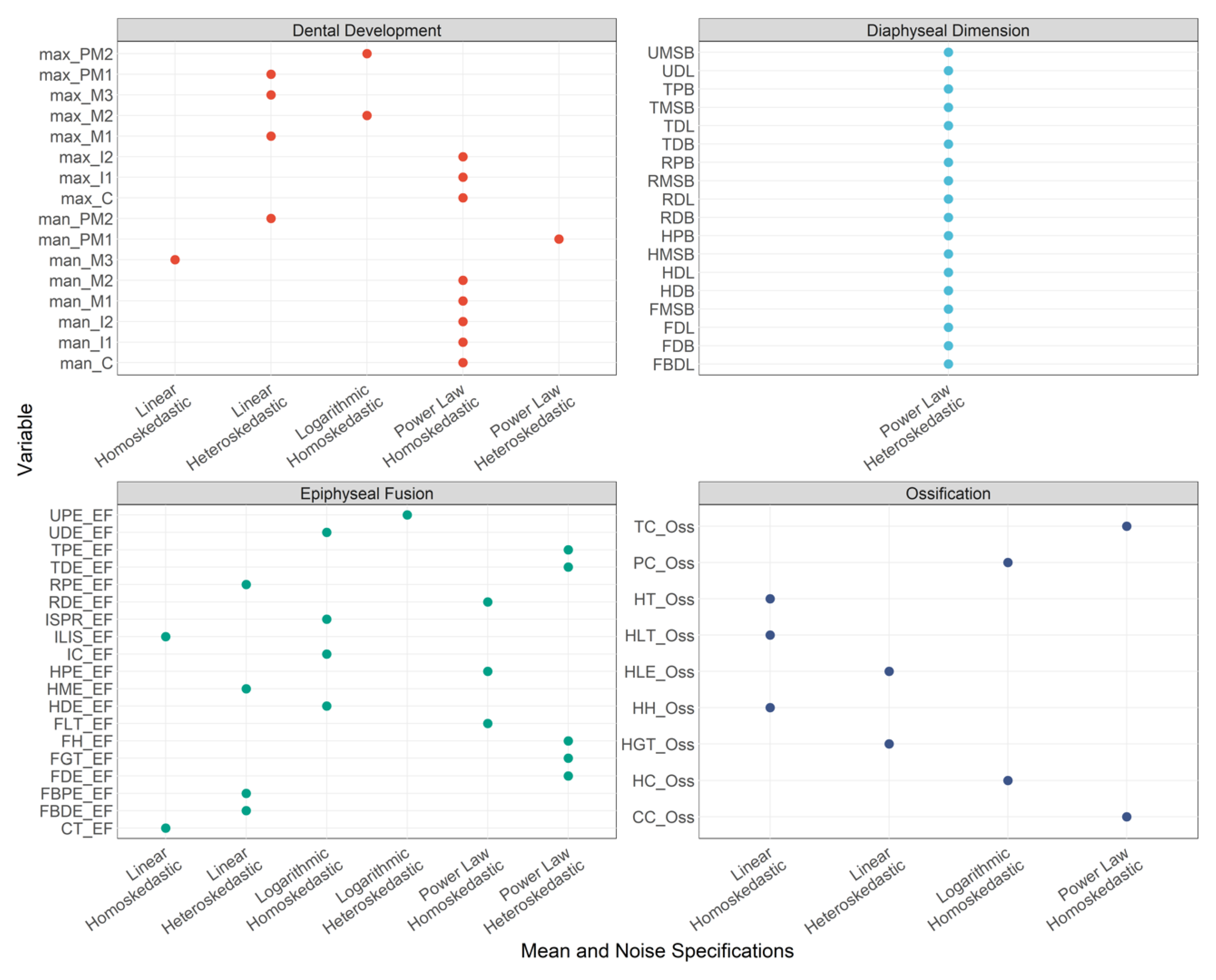
3.1. Mean and Noise Specifications

Out of the six possible parameter combinations that could be developed for the MCP models, all combinations occurred at least once in the data (Figure 5). Overall, heteroskedasticity was selected for 33 variables and homoskedasticity was selected for 29 variables. As for the mean response, 37 variables had a power law selected, seven had a logarithm selected, and 11 had a linear mean function selected. Considering all possible combinations, the least likely mean and noise specification was the logarithmic mean specification and a heteroskedastic noise specification.

The epiphyseal fusion and dental variables had more variability among the mean and noise specification combinations (

Table 6. Mean and noise specifications selected for each univariate age estimation model.

Variable	Mean Specifications	Noise Specification	Indicator Type
max_M1	Linear	Heteroskedasticity	Dental Development
max_M2	Logarithmic	Homoskedasticity	Dental Development
max_M3	Linear	Heteroskedasticity	Dental Development
max_PM1	Linear	Heteroskedasticity	Dental Development
max_PM2	Logarithmic	Homoskedasticity	Dental Development
max_C	Power Law	Homoskedasticity	Dental Development
max_I1	Power Law	Homoskedasticity	Dental Development
max_I2	Power Law	Homoskedasticity	Dental Development
man_M1	Power Law	Homoskedasticity	Dental Development
man_M2	Power Law	Homoskedasticity	Dental Development
man_M3	Linear	Homoskedasticity	Dental Development
man_PM1	Power Law	Heteroskedasticity	Dental Development
man_PM2	Linear	Heteroskedasticity	Dental Development
man_C	Power Law	Homoskedasticity	Dental Development
man_I1	Power Law	Homoskedasticity	Dental Development
man_I2	Power Law	Homoskedasticity	Dental Development
FH_EF	Power Law	Heteroskedasticity	Epiphyseal Fusion
FGT_EF	Power Law	Heteroskedasticity	Epiphyseal Fusion
FLT_EF	Power Law	Homoskedasticity	Epiphyseal Fusion
FDE_EF	Power Law	Heteroskedasticity	Epiphyseal Fusion
TPE_EF	Power Law	Heteroskedasticity	Epiphyseal Fusion
TDE_EF	Power Law	Heteroskedasticity	Epiphyseal Fusion
FBPE_EF	Linear	Heteroskedasticity	Epiphyseal Fusion
FBDE_EF	Linear	Heteroskedasticity	Epiphyseal Fusion
HH_Oss	Linear	Homoskedasticity	Ossification
HGT_Oss	Linear	Heteroskedasticity	Ossification
HLT_Oss	Linear	Homoskedasticity	Ossification
HPE_EF	Power Law	Homoskedasticity	Epiphyseal Fusion
HC_Oss	Logarithmic	Homoskedasticity	Ossification
HT_Oss	Linear	Homoskedasticity	Ossification
HLE_Oss	Linear	Heteroskedasticity	Ossification
HDE_EF	Logarithmic	Homoskedasticity	Epiphyseal Fusion
HME_EF	Linear	Heteroskedasticity	Epiphyseal Fusion
RPE_EF	Linear	Heteroskedasticity	Epiphyseal Fusion
RDE_EF	Power Law	Homoskedasticity	Epiphyseal Fusion
UPE_EF	Logarithmic	Heteroskedasticity	Epiphyseal Fusion
UDE_EF	Logarithmic	Homoskedasticity	Epiphyseal Fusion
CT_EF	Linear	Homoskedasticity	Epiphyseal Fusion
CC_Oss	Power Law	Homoskedasticity	Ossification
TC_Oss	Power Law	Homoskedasticity	Ossification
ISPR_EF	Logarithmic	Homoskedasticity	Epiphyseal Fusion
ILIS_EF	Linear	Homoskedasticity	Epiphyseal Fusion
PC_Oss	Logarithmic	Homoskedasticity	Ossification
IC_EF	Logarithmic	Homoskedasticity	Epiphyseal Fusion
FDL	Power Law	Heteroskedasticity	Diaphyseal Dimension
FMSB	Power Law	Heteroskedasticity	Diaphyseal Dimension
FDB	Power Law	Heteroskedasticity	Diaphyseal Dimension
TDL	Power Law	Heteroskedasticity	Diaphyseal Dimension
TPB	Power Law	Heteroskedasticity	Diaphyseal Dimension
TMSB	Power Law	Heteroskedasticity	Diaphyseal Dimension
TDB	Power Law	Heteroskedasticity	Diaphyseal Dimension
FBDL	Power Law	Heteroskedasticity	Diaphyseal Dimension
HDL	Power Law	Heteroskedasticity	Diaphyseal Dimension
HPB	Power Law	Heteroskedasticity	Diaphyseal Dimension
HMSB	Power Law	Heteroskedasticity	Diaphyseal Dimension
HDB	Power Law	Heteroskedasticity	Diaphyseal Dimension
RDL	Power Law	Heteroskedasticity	Diaphyseal Dimension
RPB	Power Law	Heteroskedasticity	Diaphyseal Dimension
RMSB	Power Law	Heteroskedasticity	Diaphyseal Dimension
RDB	Power Law	Heteroskedasticity	Diaphyseal Dimension
UDL	Power Law	Heteroskedasticity	Diaphyseal Dimension
UMSB	Power Law	Heteroskedasticity	Diaphyseal Dimension

, Figure 5 and Figure 6). Eleven of the dental variables had a homoskedastic noise response, and five of the dental variables had a heteroskedastic noise response. Most of the dental variables (n = 9) had a power law selected to model the shape of the data. Two dental variables had a logarithmic shape selected and five dental variables had a linear shape selected. The epiphyseal fusion and appearance of ossification centers were also evenly split between the noise response specifications; homoskedasticity was selected for 16 variables and heteroskedasticity was selected for 12 variables. In contrast to epiphyseal fusion, ossification, and dental variables, only the diaphyseal dimensions showed a consistent trend with the combination of a power law and heteroskedasticity (Table 6, Figure 5 and Figure 6).

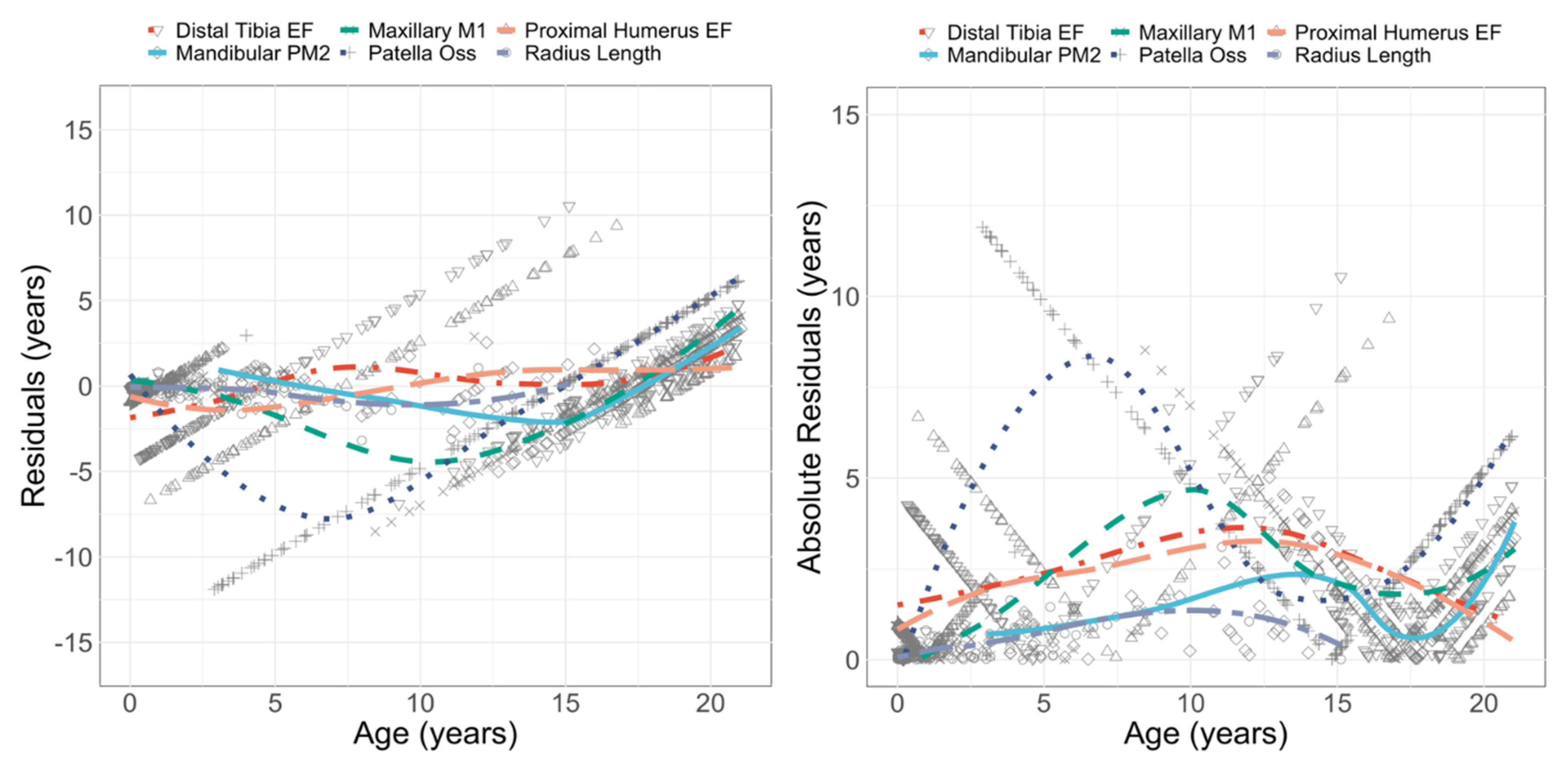
3.2. Performance: Univariate Models

The range of negative TMNLP values is −0.077 to 2.499, with a mean of 1.6 (

Table 7. Performance statistics for all univariate and multivariate age estimation models, ordered by the TMNLP. The EF models with a ‘_c’ are the collapsed, 4-Stage system. N is the sample size of the test set, which differs by variable. The model name in parentheses is the abbreviation used in the visualizations. Abbreviations: C-Dep = conditional dependence and cindep = conditional independence.

Model	N	TMNLP	% Accuracy	RMSE	Model	N	TMNLP	% Accuracy	RMSE
HDL	138	−0.077	0.96	0.688	UDE_EF_c	262	1.7934	0.93	2.066
FDL	155	0.0895	0.97	0.939	max_I1	212	1.7983	0.95	2.312
RDL	143	0.1071	0.98	0.624	RPE_EF	262	1.7994	0.94	2.153
UDL	148	0.2488	0.96	0.996	CT_EF_c	255	1.8019	0.95	2.089
TDL	159	0.2497	0.96	1.076	FH_EF_c	262	1.8039	0.94	2.839
FBDL	160	0.3034	0.96	1.205	RPE_EF_c	262	1.8081	0.94	2.209
Long Bones (C-Dep LBs)	193	0.5173	0.93	1.44	man_I1	211	1.8092	0.94	2.315
TPB	181	0.8479	0.96	1.714	man_I2	210	1.833	0.92	2.171
FMSB	157	0.8853	0.96	2.261	FLT_EF_c	261	1.837	0.96	2.141
FDB	184	0.8994	0.96	1.881	max_C	202	1.844	0.93	1.889
HPB	187	0.9079	0.97	1.508	TC_Oss_c	255	1.8712	0.96	4.453
Mixed (C-Dep 18-Var)	323	0.9216	0.91	1.164	UPE_EF	261	1.8779	0.93	2.258
Mixed (C-Dep 18-Var, Collapsed)	323	0.9434	0.9	1.167	man_C	204	1.8799	0.92	1.849
HDB	166	0.9469	0.9	2.295	UPE_EF_c	261	1.8943	0.95	2.316
TMSB	160	1.0193	0.94	2.454	TPE_EF	253	1.8945	0.93	2.977
RPB	168	1.028	0.95	2.15	max_PM2	161	1.9077	0.96	1.797
TDB	180	1.0807	0.95	1.982	HDE_EF	260	1.9122	0.93	2.473
HMSB	160	1.1064	0.92	2.932	max_M2	162	1.9192	0.95	1.679
RDB	178	1.1598	0.96	2.151	HDE_EF_c	260	1.92	0.95	2.496
Mixed (C-Indep 18-Var, Collapsed)	323	1.1965	0.82	1.203	max_PM1	174	1.9205	0.96	1.917
RMSB	161	1.2049	0.93	2.639	man_M3	117	1.9313	0.95	1.81
Mixed (C-Indep 18-Var)	323	1.2188	0.83	1.202	max_M3	116	1.9447	0.96	1.883
Proximal and Distal Epiphyses (C-Dep Prox-Dist, Collapsed)	263	1.3428	0.87	1.548	man_M2	161	1.9529	0.94	1.756
UMSB	159	1.3488	0.91	3.647	TPE_EF_c	253	1.954	0.96	3.075
Proximal and Distal Epiphyses (C-Dep Prox-Dist)	263	1.3521	0.86	1.47	man_PM1	174	1.9557	0.95	1.917
Dental (C-Dep Dental)	211	1.4132	0.84	1.161	man_PM2	161	1.9596	0.97	1.863
Epiphyseal Fusion and Ossification (C-Dep EF_Oss, Collapsed)	303	1.4995	0.79	1.533	ILIS_EF_c	261	1.9623	0.94	2.738
CC_Oss_c	263	1.5881	0.97	2.305	max_I2	194	1.9832	0.94	2.182
HPE_EF_US_all	266	1.6614	0.96	2.532	FDE_EF	256	1.9875	0.93	3.417
FBDE_EF_US_all	257	1.6654	0.94	2.793	HLE_Oss	260	2.0142	0.95	2.786
man_M1	228	1.6694	0.95	2.275	PC_Oss	257	2.0179	0.98	4.175
TDE_EF	257	1.67	0.96	2.751	ISPR_EF_c	261	2.0228	0.93	3.045
FBPE_EF	257	1.6719	0.95	2.189	FDE_EF_c	256	2.0394	0.93	3.494
max_M1	225	1.6919	0.97	2.336	Dental (C-Indep Dental)	211	2.0458	0.71	1.142
FGT_EF_c	257	1.6978	0.95	2.125	HT_Oss	261	2.0582	0.95	3.203
FBDE_EF_c	257	1.7045	0.96	2.862	IC_EF_c	112	2.0601	0.87	3.056
TDE_EF_c	257	1.7112	0.95	2.842	HLT_Oss	266	2.1379	0.96	4.988
FBPE_EF_c	257	1.7176	0.95	2.268	HGT_Oss	265	2.2141	0.94	5.907
FH_EF	262	1.7362	0.93	2.632	HC_Oss	262	2.275	0.95	6.574
RDE_EF	262	1.7365	0.91	2.971	Epiphyseal Fusion and Ossification (C-Indep Prox-Dist, Collapsed)	263	2.4014	0.7	1.841
HPE_EF_c	266	1.7381	0.96	2.639	HH_Oss	267	2.4992	0.96	7.299
UDE_EF	262	1.7674	0.93	1.998	Proximal and Distal Epiphyses (C-Indep Prox-Dist)	263	2.5076	0.71	1.712
RDE_EF_c	262	1.7714	0.92	3.021	Epiphyseal Fusion and Ossification (C-Indep EF_Oss, Collapsed)	303	2.6683	0.64	1.717
HME_EF_c	261	1.788	0.95	2.139	Long Bones (C-Indep LBs)	193	3.4524	0.56	1.217

). A smaller value indicates better test sample performance. When arranging the TMNLP from smallest to largest, all 18 diaphyseal dimensions exhibit the smallest values (<1.348) and most of the ossification variables exhibit the largest values. Primarily, a mixture of EF models and dental models have the next higher TMNLP values (~<2) (Table 7). Overall, EF models outperformed the dental variables, if evaluated at the indicator-level. Generally, if not almost always, the expanded EF data outperformed—albeit only slightly—the collapsed EF data. Mandibular and maxillary M1 are the univariate dental models that present with the smallest TMNLP values and are the only univariate dental models to be ranked in the smallest 50% of TMNLP values. The univariate dental models with the next smallest values are the mandibular and maxillary central incisors.

Long bone lengths also had the smallest RMSE values. However, in contrast to the TMNLP values, dental models had smaller RMSE values than the long bone breadth models and the EF models. Of course, there is some variability, but the general trend is true. For most variables, there are concurrent increases in both TMNLP and RMSE. However, for the dental models, there is a discordance between the performance metrics. Specifically, the dental variables exhibit higher TMNLP values with smaller RMSE values.

The percent accuracy (calculated using the test sample) for all univariate models ranged from 87% to 98%. When separated by indicator type, all indicators achieved an average accuracy of 95%, except for the expanded (7-stage) epiphyseal fusion model, which achieved a 94% accuracy (Table 7). Residual and absolute residuals plots with loess lines were generated for a few of the models that presented with the highest percent accuracy (FDL, RDL, PC_Oss, HPE_EF, TDE_EF, max_M1, man_PM2) to demonstrate discrepancies among performance metrics (Figure 7). Even though visualized models had the highest testing accuracy, there are clear discrepancies in residuals and absolute residuals depending on a variable presenting with a high or low RMSE.

The 95% CrIs per stage associated with each ordinal dental development and epiphyseal fusion and ossification univariate model are visualized in Figure 8, Figure 9 and Figure 10. The CrIs expose differential developmental trajectories for four groups of the dentition (Figure 8). The teeth that exhibit the earliest transition to development are the incisors (I1, I2), canine (C), and first molar (M1). Their trajectories are similar through the crown development and seem to diverge after the root initiation stage (Stage 6); the canine has a prolonged developmental period compared to the other teeth. Additionally, the first molar transitions through stages faster than the incisors. The second group is composed of the first and second premolars (PM1, PM2), closely followed by the second molar (M2). The third molar (M3) comprises the fourth group and has the most unique developmental trajectory. All teeth have narrower CrIs associated with the youngest ages and wider CrIs associated with the oldest ages, except the third molars. The CrIs associated with the third molars are widest at the youngest ages and narrower at the oldest ages.

The pattern across all univariate models using the collapsed EF staging system (0 to 4) is a wide 95% CrI before EF is active (Stages 0 and 1), then shorter transitions into being scored as partially fused (Stage 2), and then completely fused (Stage 4) (Figure 9). While the 95% CrI captures the variation, there is consistency across all anatomical sites that the point estimates for partial fusion (Stage 3) is between the ages of 15 and 18 years. Similarly, there is consistency in the point estimates between all anatomical sites for complete fusion (Stage 4), which is between 18 and 20 years of age (Figure 9).

More nuanced fusion patterns are exposed when the CrIs generated from the 7-stage EF data are visualized (Figure 10). For example, the distal humerus and proximal ulna and radius are some of the latest ossification sites to appear but are the earliest sites to transition through active fusion (Stages 1/2–3). In contrast, the proximal humerus appears early but has one of the later ages for active fusion. Figure 11 verifies that the CrIs associated with the EF models generated with the collapsed and expanded data yield comparable ages. However, notably, if one is working with advanced imaging and can confidently collect the data on the expanded staging system, then the more precise data collection methodology yields a more precise age estimation, particularly for stages 1/2, 2, 2/3, and 3 (Figure 10).

3.3. Performance: Multivariate and Mixed Models

The TMNLP values for the multivariate models range from 0.517 to 3.452. The multivariate models with the smallest TMNLP values are the conditionally dependent LB model and the conditionally dependent 18-Var (collapsed and expanded) mixed models, followed by the conditionally independent collapsed and expanded 18-Var models, conditionally dependent Prox-Dist, Dent, and EF_Oss models. Each conditionally dependent multivariate model exhibits a smaller TMNLP than the analogous conditionally independent model (Table 7). Notably, the mixed 18-Var conditionally independent models (collapsed and expanded) yield smaller TMNLP values than the remaining conditionally dependent and independent multivariate models.

Conditional dependence outperforms conditional independence in multivariate models based on percent accuracy and RMSE (

Table 8. K-L Bits per model. C-dep is abbreviated for conditionally dependent while C-indep is abbreviated for conditionally independent.

Models	Model Specifications	K-L bits
Mixed/18-Vars (c-dep, collapsed)	C-dep, collapsed	5.26
Mixed/18-Vars (c-indep, collapsed)	C-indep, collapsed	5.98
Mixed/18-Vars (c-dep)	C-dep	5.18
Mixed/18-Vars (c-indep)	C-indep	5.98
Long bones (c-dep)	C-dep	3.96
Long bones (c-indep)	C-indep	5.5
Epiphyseal fusion (c-dep, collapsed)	C-dep, collapsed	4.39
Epiphyseal fusion (c-indep, collapsed)	C-indep, collapsed	4.74
Dental development (c-dep)	C-dep	5.24
Dental development (c-indep)	C-indep	6.24
RDL (homoskedastic)	Homoskedasticity	4.39
RDL (heteroskedastic)	Heteroskedasticity	2.87
FDL (homoskedastic)	Homoskedasticity	4.63
FDL (heteroskedastic)	Heteroskedasticity	3.97
Man_PM2 (homoskedastic)	Homoskedasticity	4.08
Man_PM2 (heteroskedastic)	Heteroskedasticity	4.11
PC_Oss (homoskedastic)	Homoskedasticity	0.52
PC_Oss (heteroskedastic)	Heteroskedasticity	0.52

). The conditionally dependent models (with the exception of the EF_Oss model) achieved at least 84% accuracy, while the conditionally independent models (with the exception of the mixed variable model) achieved between 56% and 71%. The conditionally dependent long bone (LBs) and the mixed variable models (18 Var) are the only models to achieve an accuracy of 90% or greater.

While the LB model has the highest percent accuracy at 93% and the smallest TMNLP, the models with the smallest RMSE values are the 18 Var model and the dental model (Dent). The relationship between the larger accuracy and smaller RMSE can be seen in Figure 12. The vertical lines illustrate the CrI per individual in the test set for the LB model and Dent models; the larger CrIs were associated with the more accurate model. In contrast, the overall narrower CrIs associated with the Dent model reflects the smaller RMSE value (Figure 12). In contrast to the univariate models, almost all conditionally dependent multivariate and mixed models present with lower RMSE values; the consistent performance can be seen in the residuals and absolute residuals (Figure 13). The stability in the performance of the conditionally dependent multivariate methods across the entire age range is even more apparent when compared with the univariate models that achieved both high accuracy and low RMSE values (Figure 14).

There are two prominent results for the models that included the epiphyseal fusion and ossification data. First, there are minimal differences in the performance metrics between collapsed and expanded versions of multivariate models (e.g., Prox-Dist and EF_Oss). Second, the Prox-Dist model substantially outperforms the multivariate model that incorporates ossification data (EF_Oss).

3.4. K-L Statistic

The models with the greatest magnitude difference in the K-L bits were the diaphyseal dimensions, both at the univariate and multivariate level (Table 8, Figure 15). Because the LB models (univariate and multivariate) have a large disparity in K-L bits, the negative effects of misspecifications are clearly displayed; the conditionally independent model exhibits overconfidence. In contrast, the conditionally dependent have a broader peak with an appropriate level of confidence in the estimate. The multivariate models all have a substantial difference between the K-L bits for the conditionally dependent and independent models (Figure 15). However, the mandibular second premolar and ossification of the patella show that not all variables have large differences in the K-L bits when different specifications are modeled (Table 8), subsequently the negative effects of mismodeling are also less.

4. Discussion

The current study offers the first application of the MCP to estimate subadult age using 62 variables from all age indicators (i.e., diaphyseal dimensions, epiphyseal fusion/appearance, and dental development), and it offers immediately applicable univariate and multivariate subadult age estimation models (see Section 4.4) (Tables S1–S7). The flexible algorithm exposed the need for a variety of shape and noise parameters to appropriately capture the relationship between age indicators and age and the KL divergence statistic offered additional insight regarding the magnitude of model misspecification at the univariate and multivariate levels. The incorporation of the AIC-specified model parameters removes the need to assume a particular structure to the data, prevents concomitant misspecifications, and reduces the need to conduct post hoc analyses to correct improper modeling assumptions. The large and diverse sample of contemporary Americans split into a training sample to develop the models and an independent test sample to validate the models follows best practices and ensures the generalizability of the models and their realistic performance [53,58,59]. By properly modeling the relationships, valid ages—and the associated uncertainty—can be estimated. Therefore, comparing the performance of the current models to previously published findings may be a moot point because of the previous models’ inability to properly capture the underlying relationships.

The overwhelming majority of age indicators (56 of 62 variables) achieved a better model (e.g., smaller AIC) when the shape and noise parameters were not linear and homoskedastic, respectively (see Figure 5 and Figure 6). The diaphyseal dimensions all presented with the same combination of power law and heteroskedastic; however, no consistent combination was identified across the dental or epiphyseal fusion variables. Multivariate models that did not account for the appropriate data features produced invalid age estimates. For example, improperly assuming conditional independence yields narrow 95% CrIs and, subsequently, invalid age estimations, which can be seen with the lower percent accuracy achieved by the conditionally independent multivariate and mixed models (Table 7 and Table 8, Figure 15). This finding is what is expected to occur when assuming conditional independence when in fact the data is conditionally dependent. For conditional independence, one assumes that each variable independently informs on the posterior age distribution. Yet, a variable that is perfectly correlated with another after conditioning provides no additional information. If this is the case, and conditional independence is nevertheless assumed, posterior inference will be overconfident. Essentially, the posterior density function will be too narrow. While the long bones had the most dramatic difference in performance between the conditionally dependent and conditionally independent models (difference in KL bits = 1.54 and large difference in TMNLP of models), the same pattern was noted in the other mixed and multivariate models. For example, the difference in KL bits was 1.0 between the conditionally dependent and conditionally independent Dent models (Table 8, Figure 15).

The KL statistic facilitates further interpretation of the misspecification. The larger the bit, the more information the posterior distribution provides in relation to the prior distribution. However, a larger bit does not equate to a ‘better’ model. Rather, the KL divergence can be used to understand why a model we believe is bad is not performing well (it also can provide a quantitative measure of information gain for good models, such as to compare two univariate models). Indeed, the KL divergence can play a similar role to residuals in model evaluation. Performance metrics such as TMNLP and RMSE may indicate that a model is performing poorly, but do not directly show why that is so. Often residuals, which can be calculated either with the test or training set (the former is preferred if available), show a systematic bias or skew—for example, consistently being too high for young individuals and too low for old individuals. A plot of residuals can thus point to how the model is failing and highlight which modeling assumptions may be to blame. Similarly, if a model has poor performance but high information gain our experience suggests that an incorrect noise model has been used, usually a homoskedastic noise model when a heteroskedastic noise model is warranted.

Though the MCP offers novel flexibility in modeling parameter specifications, one limitation of the current algorithm is that there is only a maximum of six combinations for the noise (homoskedastic and heteroskedastic) and mean (linear, power law, and logarithmic) specifications. In fact, when working with ordinal data there are six possible combinations, whereas there are only two combinations available for continuous data. These data shape specifications are the most common in biological anthropology and age estimation, which is why the MCP originally incorporated them [34]. It may limit the usability of the model if variables exhibit different relationships, such as a negative heteroskedastic noise option. In fact, the third molar displayed a unique relationship with age, which was a decreasing amount of variability as age increased; this variable may be a good example of why more options would be beneficial. Related to this, the MCP model currently assumes that there is no age-dependence to the structure of the conditional correlations (i.e., the covariance matrix has no age dependence), which may not be true based on preliminary research [14].

The MCP is an algorithm that provides a platform to identify different mean and noise specifications and subsequently, facilitates an opportunity to appropriately model continuous and ordinal data. Most statistical algorithms used to develop age estimation models have not been flexible enough to model variability in both data types and structures; algorithms that have met the needs of the data in one way, may not have been able to meet the needs in another aspect. Other researchers have also argued for the benefits of flexible models, though theirs were to accommodate different informative prior age distributions, number of traits, and age threshold values [8].

4.1. Evaluating the Performance

The RMSE values appear to be at least partially related to the variable type, which can be appreciated when visualizing the CrIs along with the relationship between estimated and known chronological age (Figure 16). The number of stages associated with the ordinal data in conjunction with the age distribution informs the size of the RMSE values. Ordinal variables all saturate at the same value, meaning that at the end of the developmental process, they all reach the same stage, resulting in no variation. The number of stages, and therefore precision of the ordinal variable, impacts the RMSE values.

The binary score for the patella ossification center (PC_Oss) has a high accuracy (Table 7) because the CrIs are wide. Consequently, the RMSE value is also large. The large value associated with the RMSE is directly related to the fact that there are only two developmental stages associated with the ossification of the patella (absent and present) that cover the 21-year age range of the samples. Therefore, individuals have the same 95% CrI regardless of their age being 7 years or 18 years (Figure 17, top left). If we consider visualizations in Figure 7, we can see the impact of a binary variable slightly differently. The loess line (green, dashed line) associated with patella ossification (PC_Oss) has an obvious divergence compared to development of the mandibular second premolar (man_PM2) and radius length (RDL) because for most of the 20-year age range, it has large residuals and correspondingly high absolute residuals.

The epiphyseal fusion data is either based on a 7-stage or a 4-stage scoring system, and therefore more precise than the binary data collection strategy. The 4-stage pattern is clearly visualized in Figure 17 (top right) and its improvement in the residuals compared to PC_Oss is apparent in Figure 7. However, the metrics are only slightly different for estimates based on the 4-stage and the 7-stage scoring systems, indicating that an increase in precision for the staging system does not equate to an increase in accuracy for the resulting age estimates.

If we transition to dental development, which is also an ordinal variable but comprised of 12 developmental stages, the RMSE values are even smaller, which is reflected in the residuals (Figure 17, bottom left). Because there are more developmental stages associated with dental development, there is greater precision compared to the ossification data and epiphyseal fusion data, and as an outcome, the mandibular second premolar displays far more stability in the loess lines than the other indicators, which reflects the smaller RMSE values (Figure 7). The terminal stage in dental development is indicative of someone having completed the dental development process. Therefore, stage 12/13 (collapsed into 12 together for the current study) is only informative at the lower boundary because the upper boundary will include the oldest individuals in the sample. This is apparent in Figure 17 and in Tables S4 and S5 where the upper 95% and 99% CrIs are the age of the oldest individual in the sample. Continuous data is fundamentally the most precise data type and the inherent precision in the long bone data translates to models achieving high accuracy in combination with low error and high stability (Figure 7 and Figure 17).

These patterns in data collection methodology are apparent more so in the RMSE than the TMNLP because the RMSE is dependent on the shape and structure of the underlying data. The RMSE is appropriate when the data are linear and homoskedastic, and the current study clearly highlights that assumption is violated for many age indicators. In contrast, the TMNLP is, we think, a better metric for comparison when the posterior distributions are either non-Gaussian or are Gaussian but vary in their scale (heteroskedasticity), which is why there are less obvious indicator-type patterns in the TMNLP performance. For example, the continuous data is still distinct from ordinal data, but the stage number differences within the ordinal data is less pronounced.

The overall pattern of the TMNLP numbers makes sense (e.g., conditionally independent models perform worse), and the only real surprising result is why some of the univariate models have lower values than multivariate models. The trend for the smaller TMNLP values for the continuous univariate models is notable because the multivariate models are both a formal generalization of the individual univariate models and contain the underlying data that is used for the univariate models. All else equal, a parsimonious multivariate model could just ignore additional data if it does not improve performance [60]. So why might sub-models perform better than their more comprehensive generalizations? Almost certainly this arises from differences in the tests sets.

For the comparison to be “fair,” it must be on a comparable test dataset. Compare the best performing model in Table 7 (by TMNLP), HDL, to the 18-Var C-Dep model. The former has a TMNLP of −0.077 and RMSE of 0.688 based on 138 individuals whereas the latter has a TMNLP of 0.9216 and RMSE of 1.164 based on 323 individuals. The crucial difference between the two test samples is not the size, though, it’s that the HDL test sample has a greater proportion of young individuals (Figure 1), for which predictions are overall more accurate. This challenge—systematic differences in the test sets arising from patterns in the missingness—applies in principle to any metric (e.g., test RMSE values are also consistently lower for long bones). It is possible that if the data collection protocols had continued long bone dimension collection through epiphyseal fusion, that overall, the multivariate models would outperform all univariate models (including the long bones) in all performance metrics. For all our predictions, we have used a single prior, which is a mixture of Weibulls fit to all the ages in the training dataset. Alternatively, we might have trained separate priors on the ages available for each univariate model. Using separate priors is one way to account for the fact that there is information in the pattern of missingness. However, it is not clear to us that we want to take advantage of these patterns, though (arguably, perhaps) maybe a practitioner should want to. This is not a trivial consideration since the choice of prior can have a major impact on TMNLP and the other performance metrics.

Another possibility, which we want to acknowledge but think is less likely, is model misspecification since the model accuracy numbers fall below 95% (though the qualifications we point out above do matter). For example, as we point out elsewhere, perhaps the structure of the conditional correlation matrix is age dependent. The challenge here is that there are an infinite number of possibilities (literally) that one could nominate and check, and we have no positive evidence of a misspecification. We do, however, want to acknowledge the possibility.

4.2. Achieving High Accuracy and the Variability around 95%

The current research complements previous research that proved multivariate models outperform univariate models, in terms of greater stability across ontogeny, and less biased residuals in the estimates, e.g., [1,2,15,61]. This appears to be especially true in models based on ordinal data, where the error and bias are higher for univariate models compared to multivariate models (Table 7 and Table 8; Figure 13 and Figure 14). Some researchers, e.g., [62] have criticized multivariate techniques for (a) being more likely to overfit training data and (b) for not having crucial external validation tests. The current study used a large independent test set (n = 327) to evaluate model performance. Nevertheless, the variability around 95% accuracy speaks more directly to the concept of a model being over or underfit. It seems even more appropriate to discuss percent accuracy here as this is one performance metric that is ostensibly ‘better’ for the univariate models. Because of how the CrIs are derived, we should expect exactly 95% accuracy. Achieving higher than 95% accuracy is just as problematic as achieving lower than 95% accuracy. Essentially, if a test sample achieves 100% accuracy, it may indicate that the model is underfit and the CrIs may not be helpful in application. If a model achieves less than 95% accuracy, it may indicate the model is overfit and the CrIs may not be helpful in application. Either way, the expected outcome is to have a test accuracy around 95%; too much variability above or below 95% is suggestive of an over- or underfit model. Whether the theoretical value is exactly 95% for all models to be considered a ‘good model’ is not obvious to us; it could depend on model details and on exactly how the relevant interval is calculated.

The other component of a multivariate/mixed approach that must be considered when deciding what model one should use, is the unique developmental trajectories between each single variable and age [14,63]. Therefore, the inherent variability in the relationship makes it impossible to have a ‘best’ indicator for all of ontogeny. Epiphyseal fusion and ossification, diaphyseal dimensions, and dental development all provide complementary information that one can use to derive a more precise age estimate. In fact, variables that yield greater uncertainty in age estimates (less precision) likely have a greater improvement when combined than strongly correlated variables, which one can see when comparing univariate EF models to the multivariate EF model. For this reason, most researchers and working groups (e.g., Age Estimation Working Group or AGFAD)—especially those working with over/under maturity questions and ordinal data—support a multifactorial approach [8,59,61].

Ultimately, including more variables in an age estimation model provides more information about the individual or sample in question, and should therefore theoretically reduce the uncertainty (error) in the resulting age estimation. However, integrating more variables in the model does not necessarily always improve across all performance metrics. Indeed, accuracy is sometimes lower in multivariate models compared to univariate models, though we have already pointed out some of the pitfalls of evaluating models using percent accuracy. Additionally, using variables with strong correlations among each other and with age (e.g., the six long bone lengths), may lead to redundancy in the model and may not always lead to improved age estimates, e.g., [12]. Furthermore, adding additional variables to the fit does increase the probability of overfitting, though only if a non-parsimonious model is chosen and we should strive not to do so. Age indicators are informative of age while development is ongoing (as is the case between birth and 20 years), but the amount of information on age they carry—which can be extrapolated to their predictive ability or their contribution to the model’s performance—is related to their developmental activity, which presents with alternating periods of increase, decrease, or status. In addition to this, as mentioned previously, the very nature of these indicators and the systems used to collect them/measure them/score them will also impact their contributions to the model and the resulting age estimate.

4.3. Sex Differences and their Impact on Age Estimation

In the current study males and females were pooled for all age estimation models. Sex is often unknown in forensic cases involving skeletonized remains, and subadult sex estimation recommended or regularly performed by forensic anthropology practitioners [7,64,65]. Therefore, it was considered paramount to first build pooled-sex age estimation models to assess model performance regardless of other factors. However, male and female growth trajectories differ in their velocity and different durations in specific life history stages [66,67,68]. This results in sexual size dimorphism that is quantifiable in diaphyseal dimensions, e.g., [69,70,71] and sexual differences in timing of epiphyseal fusion timing, e.g., [72] and dental development, e.g., [6,73].

Literature positions us to argue for the logical assumption that sex-specific models would yield more precise age estimations both at the univariate and multivariate level and a pooled model would yield less precise age estimations both at the univariate and multivariate level. While our current method goals were not to build sex-specific models, we decided it important to randomly select two univariate EF variables and build sex-specific models to have empirical support rather than pure conjecture. Figure 17 visualizes the output for pooled sex, female-specific, and male-specific age estimation models using the proximal humerus (HP_EF) and the proximal tibia (TP_EF) epiphyses. The models were developed using the expanded 7-stage EF data. One can clearly see the sex-specific fusion patterns with CrIs separated by variable and stage (Figure 17). Females present with younger age ranges compared to males for each EF stage from the first appearance of the epiphysis (stage 1) through active fusion (stages 1/2 to 3); females are advanced compared to males by approximately 2 years during the active fusion stages. The pooled model has more males than females in the training sample, which is probably why the pooled model aligns with the male-specific model. Also, noteworthy is the comparable precision of the pooled model to the sex-specific models. During the process of building sex-specific models, results revealed that the 4-stage, collapsed EF data did not reveal any differential growth patterns between males and females. At least in these two variables—the proximal humerus and tibia—the 7-Stage, expanded data was required to illuminate any sexually dimorphic differences.

Interestingly, a study by Liversidge comparing age estimates based on mandibular second molar developmental stages of 946 individuals aged 3 to 16 years showed that sex-specific and pooled sex models were comparable, while the influence of the staging system and the age indicator had a greater impact on the estimates [74]. Similarly, De Tobel and colleagues [1] built sex-specific age estimation models that incorporated sexual maturation indicators (Tanner Stages) with the development of the third molars and EF of the left wrist and clavicles; the incorporation did not significantly improve age estimates. Mirroring developmental trajectories, the amount of sexual dimorphism expressed by age indicators varies according to the indicator itself and the age of the individuals/their developmental state. In view of this, sex may or may not have a substantial impact on age estimates, which is why sex-specific versus pooled sex approaches in subadult age estimation requires more explanation and may not be simple.

4.4. Accessibility and Usability

One of the more difficult obstacles is increasing the use of advanced methodological techniques. While researchers may argue that certain models are preferred, without a user-friendly interface, there is a small chance practitioners will incorporate them into use. Therefore, accessibility and usability are crucial for overall advancements in our field.

MCP-S-Age is a graphical user interface (GUI) produced using Shiny [75] in R [76]. The impetus of this user-friendly GUI is to provide a means of applying MCP univariate and multivariate models for subadult age estimation without requiring the researcher or practitioner to use R. All models presented in this manuscript and the supplementary information are currently available for immediate use through the MCP-S-Age GUI at: https://kyra-stull.shinyapps.io/mcp-s-age (accessed on 7 November 2022) and in the KidStats hub (https://kyrastull.weebly.com/kidstats.html (accessed on 7 November 2022)). Noteworthy features of this web application include model performance-based suggestions (TMNLP, RMSE, and percent accuracy) on reporting subadult skeletal age estimation, the ability to handle any number and combination of commonly used skeletal age indicators and metrics, and a downloadable report for record-keeping in forensic bench notes.

There is still a tendency of restricted access to code and/or data to develop or validate models, which has impeded application of new methods to a wide variety of researchers and practitioners. We disagree with this approach and instead make our data and protocols freely available in the SVAD Zenodo Community (https://zenodo.org/communities/svad/?page=1&size=20 (accessed on 7 November 2022)) and developed a step-by-step vignette with a downloadable script to facilitate application of the MCP to novel research questions (https://rpubs.com/elainechu/mcp_vignette (accessed on 7 November 2022)). As an additional resource and for reproducibility, we have provided a sample pipeline, step-by-step description for model optimization and selection, standalone scripts to generate further results past model optimization and selection, and an RMarkdown and HTML file demonstrating how all figures (i.e., visualizations) were produced. All files and scripts are hosted on a GitHub repository for online and offline use found here: https://github.com/ElaineYChu/fs_mcp_us (accessed on 7 November 2022).

5. Conclusions

The development of large and diverse freely available data sources, such as the SVAD, are catalysts to methodological advancements, such as the MCP, and offer opportunities to challenge theoretical underpinnings. The current study provides new, immediately applicable univariate age estimation tables for dental development and epiphyseal fusion (Tables S1–S7) and the MCP-S-Age GUI enables immediate and user-friendly applications of both univariate (all 62 variables) and multivariate models for subadult age estimation. The results exposed that mixed models outperform multivariate models, that continuous data outperforms ordinal data in both univariate and multivariate models, and models that incorporate conditional dependence outperform models that incorporate conditional independence. However, the ultimate decision of whether one should use a univariate, multivariate, or mixed model is dependent on the available data, the age of the individual, and practicalities. The authors suggest using the TMNLP in conjunction with the percent test accuracy to guide their choice though the ultimate decision is the practitioner’s.

The MCP exposed the need for a variety of mean and noise parameters to appropriately capture the relationship between age indicators and age. Beyond flexible modeling, quantification of the impact of model misspecification at the univariate and multivariate levels through KL divergence statistic offers additional insight to the relationships. By appropriately modeling the data, the groundwork is laid to further pontificate on best practices to report error as well as discuss other components that direct our interpretation, such as performance metrics and data types.

Researchers and practitioners have different needs with the introduction of new methods, but both generally require accessibility and usability. Open science initiatives have not been the overwhelming culture in biological anthropology, yet we cannot advance as a field without changing this culture. We have attempted to relieve some of the computational complexity and increase the accessibility for researchers interested in applying the MCP to future research questions. A vignette with a step-by-step tutorial as well as a template (R script) can be found here: https://rpubs.com/elainechu/mcp_vignette (accessed on 7 November 2022). A GitHub repository (https://github.com/ElaineYChu/fs_mcp_us (accessed on 7 November 2022)) detailing exact variable information, model parameters, results for the analyses herein are provided for those wishing to replicate our exact results and figures. For practitioners, we hope to increase usability by providing MCP-S-Age. This GUI offers immediate application using the United States sample and incorporates the performance metrics with all possible age estimations so practitioners can choose what best fits their needs.

The age estimation models generated in the current research include only modern individuals, therefore they are recommended for use in contemporary contexts, as historic individuals may not exhibit the same relationships between age and age indicators [77]. Additionally, the data used to generate the models is from U.S. children, therefore, it is still unknown whether the application of the age estimation models on different populations would yield valid age estimations. The intention behind the large and geographically diverse U.S. sample in the SVAD was to capture as much human variation as possible, as it is recognized that so much of growth and development is the outcome of a complex relationship between genetics and the environment. Population-specific and global subadult age estimation models using the MCP and SVAD data collected from individuals from Taiwan, Angola, South Africa, Colombia, France, the Netherlands, and Brazil are currently being generated. These models will then be incorporated into MCP-S-Age (NIJ 2017-DN-BX-0144). The authors encourage colleagues with age indicator data from diverse samples, both temporally, geographically, and/or otherwise, to upload it to the SVAD Zenodo Community so that further explorations into age estimation and specifically the impact of variation on age estimates can be made. As Coqueugniot et al. [3] suggested, data sharing can lead to improved age estimations for the entire field.

References

1. De Tobel, J.; Fieuws, S.; Hillewig, E.; Phlypo, I.; van Wijk, M.; de Haas, M.B.; Politis, C.; Verstraete, K.L.; Thevissen, P.W. Multi-Factorial Age Estimation: A Bayesian Approach Combining Dental and Skeletal Magnetic Resonance Imaging. Forensic Sci. Int. 2020, 306, 110054. [Google Scholar] [CrossRef] [PubMed]
2. Kumagai, A.; Willems, G.; Franco, A.; Thevissen, P. Age Estimation Combining Radiographic Information of Two Dental and Four Skeletal Predictors in Children and Subadults. Int. J. Leg. Med. 2018, 132, 1769–1777. [Google Scholar] [CrossRef] [PubMed]
3. Coqueugniot, H.; Weaver, T.; Houët, F. Brief Communication: A Probabilistic Approach to Age Estimation from Infracranial Sequences of Maturation. Am. J. Phys. Anthropol. 2010, 142, 655–664. [Google Scholar] [CrossRef] [PubMed]
4. Sgheiza, V. Conditional Independence Assumption and Appropriate Number of Stages in Dental Developmental Age Estimation. Forensic Sci. Int. 2022, 330, 111135. [Google Scholar] [CrossRef]
5. Duangto, P.; Janhom, A.; Prasitwattanaseree, S.; Iamaroon, A. New Equations for Age Estimation Using Four Permanent Mandibular Teeth in Thai Children and Adolescents. Int. J. Leg. Med. 2018, 132, 1743–1747. [Google Scholar] [CrossRef]
6. Esan, T.A.; Schepartz, L.A. The Timing of Permanent Tooth Development in a Black Southern African Population Using the Demirjian Method. Int. J. Leg. Med. 2019, 133, 257–268. [Google Scholar] [CrossRef]
7. Ubelaker, D.H.; Khosrowshahi, H. Estimation of Age in Forensic Anthropology: Historical Perspective and Recent Methodological Advances. Forensic Sci. Res. 2019, 4, 1–9. [Google Scholar] [CrossRef] [Green Version]
8. Konigsberg, L.W.; Frankenberg, S.R.; Sgheiza, V.; Liversidge, H.M. Prior Probabilities and the Age Threshold Problem: First and Second Molar Development. Hum. Biol. 2022, 93, 51–63. [Google Scholar] [CrossRef]
9. Sironi, E.; Vuille, J.; Morling, N.; Taroni, F. On the Bayesian Approach to Forensic Age Estimation of Living Individuals. Forensic Sci. Int. 2017, 281, e24–e29. [Google Scholar] [CrossRef]
10. Berry, S.D.; Edgar, H.J. Announcement: The New Mexico Decedent Image Database. Forensic Imaging 2021, 24, 200436. [Google Scholar] [CrossRef]
11. Stull, K.E.; Corron, L.K. The Subadult Virtual Anthropology Database (SVAD): An Accessible Repository of Contemporary Subadult Reference Data. Forensic Sci. 2022, 2, 20–36. [Google Scholar] [CrossRef]
12. Edgar, H.; Berry, D. NMDID: A New Research Resource for Biological Anthropology. Am. J. Phys. Anthropol. Suppl. 2019, 168, 166. [Google Scholar]
13. Stull, K.E.; L’Abbé, E.N.; Ousley, S.D. Using Multivariate Adaptive Regression Splines to Estimate Subadult Age from Diaphyseal Dimensions. Am. J. Phys. Anthropol. 2014, 154, 376–386. [Google Scholar] [CrossRef] [Green Version]
14. Stull, K.; Corron, L.; Price, M. Subadult Age Estimation Variables: Exploring Their Varying Roles across Ontogeny. In Remodeling Forensic Skeletal Age; Algee-Hewit, B., Kim, J., Eds.; Academic Press: Cambridge, MA, USA, 2021; pp. 49–73. [Google Scholar]
15. Corron, L.; Marchal, F.; Condemi, S.; Telmon, S. Integrating Growth Variability of the Ilium, Fifth Lumbar Vertebra, and Clavicle with Multivariate Adaptive Regression Splines Models for Subadult Age Estimation. J. Forensic Sci. 2019, 64, 34–51. [Google Scholar] [CrossRef] [Green Version]
16. Cardoso, H.F.V.; Abrantes, J.; Humphrey, L.T. Age Estimation of Immature Human Skeletal Remains from the Diaphyseal Length of the Long Bones in the Postnatal Period. Int. J. Leg. Med. 2014, 128, 809–824. [Google Scholar] [CrossRef]
17. Cunha, E.; Baccino, E.; Martrille, L.; Ramsthaler, F.; Prieto, J.; Schuliar, Y.; Lynnerup, N.; Cattaneo, C. The Problem of Aging Human Remains and Living Individuals: A Review. Forensic Sci. Int. 2009, 193, 1–13. [Google Scholar] [CrossRef]
18. National Research Council (U.S.) (Ed.) Strengthening Forensic Science in the United States: A Path Forward; National Academies Press: Washington, DC, USA, 2009; ISBN 978-0-309-13135-3. [Google Scholar]
19. Boldsen, J.; Milner, G.; Konigsberg, L.; Wood, J. Transition Analysis: A New Method for Estimating Age from Skeletons. In Paleodemography: Age Distributions from Skeletal Samples; Hoppa, R., Vaupel, J., Eds.; Cambrige University Press: Cambridge, UK, 2002; pp. 73–106. [Google Scholar]
20. DiGangi, E.; Bethard, J.; Kimmerle, E.; Konigsberg, L. A New Method for Estimating Age-At-Death From the First Rib. Am. J. Phys. Anthropol. 2009, 138, 164–176. [Google Scholar] [CrossRef]
21. Fojas, C.L.; Kim, J.; Minsky-Rowland, J.D.; Algee-Hewitt, B.F.B. Testing Inter-Observer Reliability of the Transition Analysis Aging Method on the William M. Bass Forensic Skeletal Collection. Am. J. Phys. Anthropol. 2018, 165, 183–193. [Google Scholar] [CrossRef]
22. Getz, S.M. The Use of Transition Analysis in Skeletal Age Estimation. WIREs Forensic Sci. 2020, 2, e1378. [Google Scholar] [CrossRef]
23. Godde, K.; Hens, S.M. Modeling Senescence Changes of the Pubic Symphysis in Historic Italian Populations: A Comparison of the Rostock and Forensic Approaches to Aging Using Transition Analysis. Am. J. Phys. Anthr. 2015, 156, 466–473. [Google Scholar] [CrossRef]
24. Hens, S.M.; Godde, K. New Approaches to Age Estimation Using Palatal Suture Fusion. J. Forensic Sci. 2020, 65, 1406–1415. [Google Scholar] [CrossRef] [PubMed]
25. Jooste, N.; L’Abbé, E.N.; Pretorius, S.; Steyn, M. Validation of Transition Analysis as a Method of Adult Age Estimation in a Modern South African Sample. Forensic Sci. Int. 2016, 266, 580.e1–580.e7. [Google Scholar] [CrossRef] [PubMed]
26. Sironi, E.; Taroni, F. Bayesian Networks for the Age Classification of Living Individuals: A Study on Transition Analysis. J. Forensic Sci. Med. 2015, 1, 124–132. [Google Scholar] [CrossRef]
27. Tangmose, S.; Thevissen, P.; Lynnerup, N.; Willems, G.; Boldsen, J. Age Estimation in the Living: Transition Analysis on Developing Third Molars. Forensic Sci. Int. 2015, 257, 512.e1–512.e7. [Google Scholar] [CrossRef] [PubMed] [Green Version]
28. Konigsberg, L.; Herrmann, N.; Wescott, D.; Kimmerle, E. Estimation and Evidence in Forensic Anthropology: Age-at-Death. J. Forensic Sci. 2008, 53, 541–557. [Google Scholar] [CrossRef]
29. Konigsberg, L.W.; Frankenberg, S.R. Estimation of Age Structure in Anthropological Demography. Am. J. Phys. Anthropol. 1992, 89, 235–256. [Google Scholar] [CrossRef]
30. Milner, G.R.; Boldsen, J.L. Transition Analysis: A Validation Study with Known-Age Modern American Skeletons. Am. J. Phys. Anthropol. 2012, 148, 98–110. [Google Scholar] [CrossRef]
31. Nikita, E.; Nikitas, P. Skeletal Age-at-Death Estimation: Bayesian versus Regression Methods. Forensic Sci. Int. 2019, 297, 56–64. [Google Scholar] [CrossRef]
32. Konigsberg, L.W. Multivariate Cumulative Probit for Age Estimation Using Ordinal Categorical Data. Ann. Hum. Biol. 2015, 42, 368–378. [Google Scholar] [CrossRef]
33. Fieuws, S.; Willems, G.; Larsen-Tangmose, S.; Lynnerup, N.; Boldsen, J.; Thevissen, P. Obtaining Appropriate Interval Estimates for Age When Multiple Indicators Are Used: Evaluation of an Ad-Hoc Procedure. Int. J. Leg. Med. 2015, 130, 489–499. [Google Scholar] [CrossRef]
34. Stull, K.; Chu, E.; Corron, L.; Price, M. Mixed Cumulative Probit: A Multivariate Generalization of Transition Analysis That Accommodates Variation in the Shape, Spread, and Structure of Data. R. Soc. Open Sci. 2022. submitted. [Google Scholar]
35. Allison, P.A.; Bottjer, D.J. Taphonomy: Bias and Process Through Time. In Taphonomy: Process and Bias Through Time; Allison, P.A., Bottjer, D.J., Eds.; Aims & Scope Topics in Geobiology Book Series; Springer Netherlands: Dordrecht, The Netherlands, 2011; pp. 1–17. ISBN 978-90-481-8643-3. [Google Scholar]
36. Stodder, A.L.W. Taphonomy and the Nature of Archaeological Assemblages. In Biological Anthropology of the Human Skeleton; John Wiley & Sons, Ltd.: Hoboken, NJ, USA, 2018; pp. 73–115. ISBN 978-1-119-15164-7. [Google Scholar]
37. Berry, S.D.; Edgar, H.J.H. Extracting and Standardizing Medical Examiner Data to Improve Health. AMIA Jt. Summits Transl. Sci. Proc. 2020, 2020, 63–70. [Google Scholar]
38. Edgar, H.; Daneshvari Berry, S.; Moes, E.; Adolphi, N.; Bridges, P.; Nolte, K. New Mexico Decedent Image Database (NMDID); Office of the Medical Investigator, University of New Mexico: Albuquerque, NM, USA, 2020. [Google Scholar] [CrossRef]
39. Ousley, S. A Radiographic Database for Estimating Biological Parameters in Modern Subadults; Final Technical Report, National Institute of Justice Award Number 2008-DN-BX-K152; Mercyhurst University: Erie, PA, USA, 2013. Available online: https://ncjrs.gov/pdffiles1/nij/grants/242697.pdf (accessed on 7 November 2022).
40. Stull, K.E.; Wolfe, C.A.; Corron, L.K.; Heim, K.; Hulse, C.N.; Pilloud, M.A. A Comparison of Subadult Skeletal and Dental Development Based on Living and Deceased Samples. Am. J. Phys. Anthropol. 2021, 175, 36–58. [Google Scholar] [CrossRef]
41. Spake, L.; Hoppa, R.D.; Blau, S.; Cardoso, H.F.V. Lack of Biological Mortality Bias in the Timing of Dental Formation in Contemporary Children: Implications for the Study of Past Populations. Am. J. Phys. Anthropol. 2021, 174, 646–660. [Google Scholar] [CrossRef]
42. Spake, L.; Hoppa, R.D.; Blau, S.; Cardoso, H.F.V. Biological Mortality Bias in Diaphyseal Growth of Contemporary Children: Implications for Paleoauxology. Am. J. Biol. Anthropol. 2022, 178, 89–107. [Google Scholar] [CrossRef]
43. Stull, K.; Corron, L.K. Subadult Virtual Anthropology Database (SVAD) Data Collection Protocol: Epiphyseal Fusion, Diaphyseal Dimensions, Dental Development Stages, Vertebral Neural Canal Dimensions. Zenodo 2021. [Google Scholar] [CrossRef]
44. Corron, L.K.; Stock, M.K.; Cole, S.J.; Hulse, C.N.; Garvin, H.M.; Klales, A.R.; Stull, K.E. Standardizing Ordinal Subadult Age Indicators: Testing for Observer Agreement and Consistency across Modalities. Forensic Sci. Int. 2021, 320, 110687. [Google Scholar] [CrossRef]
45. Stull, K.; Corron, L. SVAD_US (1.0.0) [Data Set]. Zenodo 2021. [Google Scholar] [CrossRef]
46. AlQahtani, S.J.; Hector, M.P.; Liversidge, H.M. Brief Communication: The London Atlas of Human Tooth Development and Eruption. Am. J. Phys. Anthr. 2010, 142, 481–490. [Google Scholar] [CrossRef]
47. Corron, L.K.; Broehl, K.A.; Chu, E.Y.; Vlemincq-Mendieta, T.; Wolfe, C.A.; Pilloud, M.A.; Scott, G.R.; Spradley, M.K.; Stull, K.E. Agreement and Error Rates Associated with Standardized Data Collection Protocols for Skeletal and Dental Data on 3D Virtual Subadult Crania. Forensic Sci. Int. 2022, 334, 111272. [Google Scholar] [CrossRef]
48. Colman, K.L.; de Boer, H.H.; Dobbe, J.G.G.; Liberton, N.P.T.J.; Stull, K.E.; van Eijnatten, M.; Streekstra, G.J.; Oostra, R.-J.; van Rijn, R.R.; van der Merwe, A.E. Virtual Forensic Anthropology: The Accuracy of Osteometric Analysis of 3D Bone Models Derived from Clinical Computed Tomography (CT) Scans. Forensic Sci. Int. 2019, 304, 109963. [Google Scholar] [CrossRef] [PubMed]
49. Colman, K.L.; Dobbe, J.G.G.; Stull, K.E.; Ruijter, J.M. The Geometrical Precision of Virtual Bone Models Derived from Clinical Computed Tomography Data for Forensic Anthropology. Int. J. Leg. Med. 2017, 131, 1155–1163. [Google Scholar] [CrossRef]
50. Garvin, H.M.; Stock, M.K. The Utility of Advanced Imaging in Forensic Anthropology. Acad. Forensic Pathol. 2016, 6, 499–516. [Google Scholar] [CrossRef] [PubMed]
51. Stock, M.K.; Garvin, H.M.; Corron, L.K.; Hulse, C.N.; Cirillo, L.E.; Klales, A.R.; Colman, K.L.; Stull, K.E. The Importance of Processing Procedures and Threshold Values in CT Scan Segmentation of Skeletal Elements: An Example Using the Immature Os Coxa. Forensic Sci. Int. 2020, 309, 110232. [Google Scholar] [CrossRef] [PubMed]
52. Kuhn, M. Caret: Classification and Regression Training; Astrophysics Source Code Library, 2015. 1505.003. Available online: https://www.semanticscholar.org/paper/caret%3A-Classification-and-Regression-Training-Kuhn/258c7e3242b91e02e092e77e058f6275ba52b12d (accessed on 31 October 2022).
53. Valsecchi, A.; Irurita Olivares, J.; Mesejo, P. Age Estimation in Forensic Anthropology: Methodological Considerations about the Validation Studies of Prediction Models. Int. J. Leg. Med. 2019, 133, 1915–1924. [Google Scholar] [CrossRef] [Green Version]
54. Gelman, A.; Hwang, J.; Vehtari, A. Understanding Predictive Information Criteria for Bayesian Models. Stat. Comput. 2014, 24, 997–1016. [Google Scholar] [CrossRef]
55. Gneiting, T. Making and Evaluating Point Forecasts. J. Am. Stat. Assoc. 2011, 106, 746–762. [Google Scholar] [CrossRef] [Green Version]
56. Corron, L. Juvenile Age Estimation in Physical Anthropology: A Critical Review of Existing Methods and the Application of Two Standardised Methodological Approaches. Ph.D. Thesis, Aix-Marseille University, Marseille, France, 2016; 870p. [Google Scholar]
57. Milner, G.; Boldsen, J. Skeletal Age Estimation: Where Are We and Where Should We Go? In A Companion to Forensic Anthropology; Dirkmaat, D., Ed.; Wiley-Blackwell: Malden, MA, USA, 2012. [Google Scholar]
58. Corron, L.; Marchal, F.; Condemi, S.; Adalian, P. A Critical Review of Sub-Adult Age Estimation in Biological Anthropology: Do Methods Comply with Published Recommendations? Forensic Sci. Int. 2018, 288, 328.e1–328.e9. [Google Scholar] [CrossRef]
59. Schmeling, A.; Garamendi González, P.; Prieto, J.; Landa, M. Forensic Age Estimation in Unaccompanied Minors and Young Living Adults. In Forensic Medicine from Old Problems to New Challenges; Vieira, D.N., Ed.; IntechOpen: London, UK, 2011; ISBN 978-953-307-262-3. [Google Scholar]
60. Stull, K.; Armelli, K. Combining Variables to Improve Subadult Age Estimation. Forensic Anthropol. 2020, 3, 203–223. [Google Scholar] [CrossRef]
61. Štern, D.; Payer, C.; Giuliani, N.; Urschler, M. Automatic Age Estimation and Majority Age Classification From Multi-Factorial MRI Data. IEEE J. Biomed. Health Inform. 2019, 23, 1392–1403. [Google Scholar] [CrossRef]
62. Cardoso, H.F.V.; Vandergugten, J.M.; Humphrey, L.T. Age Estimation of Immature Human Skeletal Remains from the Metaphyseal and Epiphyseal Widths of the Long Bones in the Post-Natal Period. Am. J. Phys. Anthr. 2017, 162, 19–35. [Google Scholar] [CrossRef]
63. Wolfe, C.; Chu, E.; Corron, L.; Price, M.; Stull, K. Advances in Subadult Age Estimation: Using Information Theory to Explore the Relationship Between Growth Indicators and Age. In Proceedings of the 91st Annual Meeting, Denver, CO, USA, 23–26 March 2022. [Google Scholar]
64. Stull, K.; Cole, S.; Cirillo, L.; Hulse, C. Subadult Sex Estimation. In Sex Estimation of the Human Skeleton: History, Methods, and Emerging Techniques; Academic Press: Cambridge, MA, USA, 2020; p. 424. [Google Scholar]
65. ANSI/ASB Standard 0090; Standard for Sex Estimation in Forensic Anthropology. Academy Standards Board: Colorado Springs, CO, USA, 2019.
66. Badyaev, A.V. Growing Apart: An Ontogenetic Perspective on the Evolution of Sexual Size Dimorphism. Trends Ecol. Evol. 2002, 17, 369–378. [Google Scholar] [CrossRef]
67. Bogin, B. Patterns of Human Growth, 3rd ed.; Cambridge Studies in Biological and Evolutionary Anthropology; Cambridge University Press: Cambridge, UK, 2020; ISBN 978-1-108-43448-5. [Google Scholar]
68. Hauspie, R.; Roelants, M. Adolescent Growth. In Human Growth and Development; Cameron, N., Bogin, B., Eds.; Elsevier: New York, NY, USA, 2012; pp. 57–79. [Google Scholar]
69. Krüger, G.; L’Abbe, E.; Stull, K. Sex Estimation from the Long Bones of Modern South Africans. Int. J. Leg. Med. 2017, 131, 275–285. [Google Scholar] [CrossRef]
70. Stull, K.; L’Abbe, E.; Ousley, S. Subadult Sex Estimation from Diaphyseal Dimensions. Am. J. Phys. Anthr. 2017, 163, 64–74. [Google Scholar] [CrossRef] [PubMed]
71. Spradley, M.; Jantz, R. Sex Estimation in Forensic Anthropology: Skull versus Postcranial Elements. J. Forensic Sci. 2011, 56, 289–296. [Google Scholar] [CrossRef]
72. Scheuer, L.; Black, S. Developmental Juvenile Osteology; Elsevier Academic Press: New York, NY, USA, 2000. [Google Scholar]
73. Liversidge, H.M.; Peariasamy, K.; Folayan, M.O.; Adeniyi, A.O.; Ngom, P.I.; Mikami, Y.; Shimada, Y.; Kuroe, K.; Tvete, I.F.; Kvaal, S.I. A Radiographic Study of the Mandibular Third Molar Root Development in Different Ethnic Groups. J. Forensic Odontostomatol. 2017, 35, 97–108. [Google Scholar]
74. Liversidge, H.M. Controversies in Age Estimation from Developing Teeth. Ann. Hum. Biol. 2015, 42, 397–406. [Google Scholar] [CrossRef]
75. Chang, W.; Cheng, J.; Allaire, J.; Sievert, C.; Schloerke, B.; Xie, Y.; Allen, J.; McPherson, J.; Dipert, A.; Borges, B. Shiny: Web Application Framework for R. 2021. Available online: https://shiny.rstudio.com/ (accessed on 7 November 2022).
76. R Core Team. R: A Language and Environment for Statistical Computing; R Foundation for Statistical Computing: Vienna, Austria, 2021. [Google Scholar]
77. Heuze, Y.; Cardoso, F. Testing the Quality of Nonadult Bayesian Dental Age Assessment Methods to Juvenile Skeletal Remains: The Lisbon Collection Children and Secular Trend Effects. Am. J. Phys. Anthropol. 2007, 135, 275–283. [Google Scholar] [CrossRef]
Figure 1. Visualization of available data per chronological age in the United States sample queried from the SVAD. The color is indicative of the percent of data available out of a total of 62 age indicators that were collected. Therefore, the darker blue indicates no data is available for any individual per chronological age and the darker red indicates all individuals have data available at that age. Abbreviations for the variables can be found in Tables 2–4.
Forensicsci 02 00055 g001
Figure 2. Age and sex distributions of the sample separated by the training and testing subsets.
Forensicsci 02 00055 g002
Figure 3. Epiphyseal scoring system by anatomical location.
Forensicsci 02 00055 g003
Figure 4. Diaphyseal dimensions collected per individual. Please refer to Table 4 for the abbreviations.
Forensicsci 02 00055 g004
Figure 5. Parameter specifications selected for all univariate models and visualized by indicator type. The area of the points is proportional to the number of models of each type. The x-axis separates by noise model and the y-axis separates by mean model. The colors indicate the variable type (the legend is above the plot).
Forensicsci 02 00055 g005
Figure 6. Parameter specifications per variable, separated by indicator type. Each of the four sub-plots is for a different variable type (Dental Development, Diaphyseal Dimension, Epiphyseal Fusion, and Ossification). The x-axis of each subplot is the model type and the y-axis of each subplot is the variable.
Forensicsci 02 00055 g006
Figure 7. Loess lines expose the trends in the residuals (left) and absolute residuals (right) of a few of the univariate models that had high accuracy and large RMSE values.
Forensicsci 02 00055 g007
Figure 8. 95% credible intervals (lines) and mean point estimate (circles) of the univariate dental models for each dental development stage by tooth type. Blue lines and dots correspond to the maxillary teeth; black lines correspond to the mandibular teeth.
Forensicsci 02 00055 g008
Figure 9. 95% credible intervals (lines) and point estimates (circle) per stage of the univariate epiphyseal fusion models for each proximal and distal long bone epiphysis following. The visualized models were generated used the collapsed data (4-stages).
Forensicsci 02 00055 g009
Figure 10. 95% credible intervals (line) and mean (circle) per stage for the proximal and distal epiphyses models. The visualized models were generated used the expanded data (7-stages).
Forensicsci 02 00055 g010
Figure 11. Overlaid 95% credible intervals of the 4-stage (blue, solid) EF models and the 7-stage EF models (black, dashed).
Forensicsci 02 00055 g011
Figure 12. Point estimate of age (point) and 95%CrI (vertical error bar) regressed on known age for the conditionally dependent long bones model (black) and conditionally dependent dental model (blue). Note the more precise but inaccurate multivariate dental model and the more accurate but less precise long bone model.
Forensicsci 02 00055 g012
Figure 13. Loess lines expose the trends in the residuals (top) and absolute residuals (bottom) of four multivariate/mixed models.
Forensicsci 02 00055 g013
Figure 14. Loess lines expose the trends in the residuals (top) and absolute residuals of four univariate models and the conditionally dependent 18-Var multivariate model.
Forensicsci 02 00055 g014
Figure 15. Results for the same 8-year-old were visualized for each model to illustrate the relationship between true age and the posterior density region associated with each model. Each density line represents different model specifications, both at the univariate level (heteroskedasticity [hetero]/homoskedasticity [homo]) and at the multivariate level (conditional dependence [C-Dep]/conditional independence [C-Indep]). Top Left: comparison of seven multivariate and univariate models; Top Right: the long bone (LBs) multivariate model and the univariate radius length model; Bottom Left: multivariate dental development (Dent) model; Bottom Right: 18-variable (18-Var) mixed multivariate model.
Forensicsci 02 00055 g015
Figure 16. Predicted age of the test sample regressed on known age of the test sample for the patella ossification (top left), the epiphyseal fusion of the distal tibia (top right) (collapsed 4-stage system), maxillary first molar (bottom left), and radius diaphyseal length (bottom right) model. The circles are the point estimates, and the straight vertical line is the associated 95% CrI.
Forensicsci 02 00055 g016
Figure 17. Sex-specific and pooled sex age estimation models using HPE_EF (left) and TP_EF (right). The CrIs and point estimate are provided per model type (pooled sexes, female-specific and male-specific) and EF stage.
Forensicsci 02 00055 g017