R-Matrix Theory in a Semiconductor Quantum Device: Weak Formulation and Current Conserving Approximations

Abstract

In a series of previous publications an R-matrix approach was developed to describe transport in N-pole quantum devices in the Landauer–Büttiker formalism. Central quantities in this formalism are the transmission coefficients occurring in coherent scattering functions ranging throughout the device. Here we develop the weak formulation version of this approach. It allows to introduce systematically approximations that reduce the exact problem to suitable matrix equations that can be solved on the computer. As a major advantage of our method any approximation found in the weak formulation approach to the R-matrix is current conserving by construction. Here the essential step is the representation of the current S-matrix by a Cayley transform. Restricting us to the one-dimensional case we find that the R-matrix in weak formulation generates a real symmetric Cayley transform by construction. From general theory it follows immediately that the current is conserved.

1. Introduction

The understanding and the practical evaluation of transmission and reflection coefficients in scattering functions play a crucial role in quantum transport. The transmission coefficients are the central quantities in the very frequently used Landauer–Büttiker formalism, pioneered by Frenkel [1], Ehrenberg and Hönl [2], Landauer [3,4], Tsu and Esaki [5], Fisher and Lee [6], and progressed to its present form by Büttiker [7,8,9].

For formal developments as well as for numerical and analytical evaluations of the transmission coefficients in transistor devices we have employed the R-matrix method in a number of papers. Examples include conventional MOSFETs [10], nanowire transistors [11], spin-FETs [12], quantum logic gates [13], SOI transistors [14], and the two-channel transistor as a proposal for a new device architecture based on SOI technology [15]. This R-matrix method was introduced by Wigner and Eisenbud and has been widely used in atomic and nuclear physics (for reviews see Refs. [16,17]). A similar method was developed by Kapur and Peierls [18]. The application of the R-matrix technique to mesoscopic semiconductor systems has been demonstrated by Smrčka [19] for one-dimensional structures.

In this paper we demonstrate, as a major advantage, that the R-matrix technique allows the systematic introduction of current-conserving approximations for transmission coefficients. As a standard tool to introduce approximations we use the method by Galerkin (see Chapter 14 of [20]) to cast the Schrödinger equation in a weak formulation. While any exact solution to the time-independent Schrödinger equation conserves the current, this cannot be expected in general for an approximative solution so that unphysical artifacts may arise.

In the weak formulation the wave function is assumed to be a linear combination of basis functions (‘LCAO approximation’) which are chosen appropriately. An important example is the finite element method in which what are known as hat functions are used as basis functions (Section 5). The application of the weak formulation method to the Schrödinger scattering problem was demonstrated in the quantum transmitting boundary method by Lent and Kirkner [21,22,23,24,25]. This method leads to a set of linear equations for the calculation of the LCAO approximation of the scattering functions (‘direct calculation’, Appendix A). From this set of linear equations, it is straightforward to construct the R-matrix in weak formulation (Section 3). Since the R-matrix is real and symmetric, a standard eigenvector expansion of the R-matrix in weak formulation is derived in Section 4. Applying a standard variational analysis in Appendix C the eigenvectors in the eigenvector expansion are shown to be the best possible LCAO approximation of the Wigner–Eisenbud states which result from Neumann boundary conditions in the strong formulation. With a standard procedure the S-matrix containing the transmission coefficients can be calculated (Appendix B). As usual, in the R-matrix theory the R- and S-matrix can be constructed easily for all energies in the eigenvector expansion.

As shown in the strong formulation in [26], the essential step is the representation of the current S-matrix by a Cayley transform. The current S-matrix is a modification of the S-matrix suitable for the description of quantum currents rather than wave functions. The general theory yields that if and only if the Cayley transform of the current S-matrix is skew-symmetric, current conservation follows [27,28]. Restricting ourselves for clarity to the one-dimensional case, we find that the R-matrix in weak formulations generates real symmetric Cayley transforms of the current S-matrix without exception, i.e., any weak formulation approximation to the R-matrix leads to a current-conserving S-matrix.

Finally in Section 6 we consider an analytical example to find that in this case the ‘direct calculation’ completely fails to preserve current conservation while the R-matrix method preserves it.

2. Schrödinger Scattering Problem in One Dimension: Current R-Matrix and Current S-Matrix

We consider the Schrödinger scattering problem in one dimension

$$\begin{array}{ccc}& & \left[-{\displaystyle \frac{{\hslash }^2}{2m}}{\displaystyle \frac{d^2}{d{x}^2}}+V\left(x\right)-E\right]\Psi \left(x\right)=0\hfill \\ & \iff & \left[{\displaystyle \frac{d^2}{d{x}^2}}-v\left(x\right)+ϵ\right]\Psi \left(x\right)=0,\hfill \end{array}$$

(1)

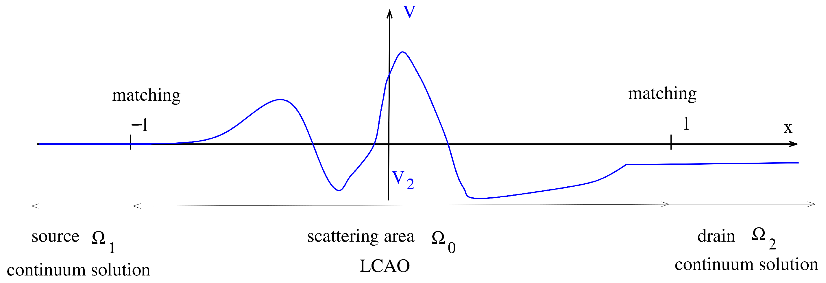
with $ϵ=2mE/{\hslash }^2$ and $v\left(x\right)=2mV\left(x\right)/{\hslash }^2$. As shown in Figure 1 the potential exhibits the asymptotics $V(x\le -l)=0$ in the source ${\Omega }_1$ and $V(x\ge l)=V_2=-e{U}_D$ in the drain ${\Omega }_2$. We approximate the wave function in the the scattering area ${\Omega }_0=⟨-l,l⟩$ as an LCAO-type linear combination

$$\Psi (x\in {\Omega }_0)=\sum _{j=1}^n{\Psi }^j{\Phi }_j\left(x\right)$$

(2)

of n appropriately chosen real basis functions ${\Phi }_j\left(x\right)$. We cast Equation (1) in weak formulation according to the method by Galerkin [20] and project onto the space of wave functions spanned by the basis functions ${\Phi }_j$ by multiplication of (1) with ${\Phi }_j$ and after subsequent partial integration we require

$${\left[{\Phi }_j\left(x\right){\Psi }^{\prime }\left(x\right)\right]}_{-l}^l=\sum _{j^{\prime }=1}^n\left(h_{j{j}^{\prime }}-ϵb_{j{j}^{\prime }}\right){\Psi }^{j^{\prime }}.$$

(3)

Here we define the Hamilton matrix

$$h_{j{j}^{\prime }}={\int }_{-l}^{l}dx\left[{\Phi }_j^{\prime }\left(x\right){\Phi }_{j^{\prime }}^{\prime }\left(x\right)+{\Phi }_j\left(x\right)v\left(x\right){\Phi }_{j^{\prime }}\left(x\right)\right]$$

(4)

and the overlap matrix

$$b_{j{j}^{\prime }}={\int }_{-l}^{l}dx{\Phi }_j\left(x\right){\Phi }_{j^{\prime }}\left(x\right)$$

(5)

which are both real symmetric $n\times n$ matrices. As demonstrated in Appendix A from Equation (3) one can derive a set of linear inhomogeneous equations to determine the transmission coefficients, as has been done in the quantum transmitting boundary method. Here the transmission coefficients are introduced in the inhomogeneity on the left side of (3) using standard matching conditions at the surface of the scattering area (here $l^{\pm }\equiv l\pm \xi$, $\xi >0$, $\xi \to 0$)

$$\Psi (\pm l^{-})=\Psi (\pm l^{+})\equiv \Psi (\pm l)\mathrm{defining}{\Psi }_1=\Psi (-l)\mathrm{and}{\Psi }_2=\Psi \left(l\right).$$

(6)

At $x=\pm l^{-}$ the expansion (2) is used. At $x=\pm l^{+}$ the expansion of the wave function in the lead ${\Omega }_s$ is used, where we write

$$\Psi (x\in {\Omega }_s)={\Psi }_s^{in}exp(-i{k}_s{z}_s)+{\Psi }_s^{out}exp\left(i{k}_s{z}_s\right).$$

(7)

where we have $k_s=\sqrt{ϵ-v_s}$ with $v_s=2m{V}_s/{\hslash }^2$. The channel coordinates are defined as $z_1=-(x+l)$ and $z_2=-(x-l)$. Here $z_s$ vanishes at the interfaces $x=x_s={(-1)}^{s}l$ between the leads ${\Omega }_s$ and ${\Omega }_0$. The channel coordinate grows towards the interior of the leads so the components $\propto exp\left(i{k}_s{z}_s\right)$ are the outgoing components. We furthermore have the matching of the outward directed normal derivative

$${\Psi }^S(\pm l^{-})={\Psi }^S(\pm l^{+})\equiv {\Psi }^S(\pm l)$$

(8)

defining

$${\Psi }_1^S={\Psi }^S(-l)=-{\Psi }^{\prime }(-l)\mathrm{and}{\Psi }_2^S={\Psi }^S\left(l\right)={\Psi }^{\prime }\left(l\right).$$

(9)

In this paper we take a route different from that in Appendix A and define the R-matrix from which the S-matrix can be calculated which in turn contains the transmission coefficients: The generalized R-matrix is defined by the relationship

$${\Psi }_s=\sum _s{R}_{s{s}^{\prime }}^{\alpha }{\Psi }_{s^{\prime }}^S$$

(10)

(see definitions for ${\Psi }_s$ and ${\Psi }_s^S$, $s=1,2$ in Equations (6) and (9)). The R-matrix is constructed in weak formulation in Section 3. Furthermore, from (7) we define the two-component vectors

$${\overrightarrow{\Psi }}^{in}=\left(\begin{array}{c}{\Psi }_1^{in}\\ \\ {\Psi }_2^{in}\end{array}\right)\mathrm{and}{\overrightarrow{\Psi }}^{out}=\left(\begin{array}{c}{\Psi }_1^{out}\\ \\ {\Psi }_2^{out}\end{array}\right)$$

(11)

as well as the S-matrix as the linear mapping

$${\overrightarrow{\Psi }}^{out}=S{\overrightarrow{\Psi }}^{in}\mathrm{with}S=\left(\begin{array}{cc}{r}^1& t^2\\ t^1& r^2\end{array}\right).$$

(12)

To arrive at (12) we write for the source-incident scattering state ${\Psi }^1$ choosing in (7) ${\Psi }_1^{in}=1$ and ${\Psi }_2^{in}=0$

$${\Psi }^1\left(x\right)=\left\{\begin{array}{cc}\exp \left(i{k}_1{z}_1\right)+r^{1}exp(-i{k}_1{z}_1)\hfill & \mathrm{for} x\le -l\hfill \\ t^{1}exp\left(i{k}_2{z}_2\right)\hfill & \mathrm{for} x\ge l.\hfill \end{array}\right.$$

(13)

For the drain incident state ${\Psi }^2$ with ${\Psi }_2^{in}=1$ and ${\Psi }_1^{in}=0$ we write

$${\Psi }^2\left(x\right)=\left\{\begin{array}{cc}{t}^2\exp (-i{k}_1{z}_1)\hfill & \mathrm{for} x\le -l\hfill \\ \exp (-i{k}_2{z}_2)+r^{2}exp\left(i{k}_2{z}_2\right)\hfill & \mathrm{for} x\ge l.\hfill \end{array}\right.$$

(14)

In Appendix B it is shown that the S-matrix is given by

$$S=-{\displaystyle \frac{1+iRk}{1-iRk}}.$$

(15)

Here we define the further two-component matrices ${\left(R\right)}_{s{s}^{\prime }}=R_{s{s}^{\prime }}$ and ${\left(k\right)}_{s{s}^{\prime }}={\delta }_{s{s}^{\prime }}{k}_{s^{\prime }}$.

In Ref. [29] it was shown that in the Landauer–Büttiker formalism the transport properties are rather obtained from the current S-matrix than from the S-matrix itself. For the current S-matrix we obtain

$$\begin{array}{c}\hfill \tilde{S}=k^{1/2}S{k}^{-1/2}=-{\displaystyle \frac{1+i\Omega }{1-i\Omega }}\end{array}$$

(16)

which takes the form of a Cayley transformation where the Cayley transform is the current R-matrix

$$\Omega =k^{1/2}R{k}^{1/2}.$$

(17)

In the one-dimensional case R is real and symmetric and it results that $\Omega$ is also real and symmetric at $ϵ\ge 0$. Since the Cayley transform of the current S-matrix is real and symmetric, it follows that $\tilde{S}$ is unitary [27,28] from which the conservation of the current is obtained as was discussed in Ref. [26] for the general case. In the one-dimensional case this can be easily seen writing from (12) for the current S-matrix

$$\tilde{S}=\left(\begin{array}{cc}{r}^1& k_1{t}^2{k}_2^{-1/2}\\ k_2{t}^1{k}_1^{-1/2}& r^2\end{array}\right).$$

(18)

If $\tilde{S}$ is now unitary one has, for example, for the first column vector

$$\begin{array}{ccc}& & |r^1{|}^2+{\displaystyle \frac{k_2}{k_1}}{|t^1|}^2=1\hfill \\ & \iff & k_1|r^1{|}^2+k_2{|t^1|}^2=k_1\hfill \\ & \iff & I^{ref}\left({\Psi }_1\right)+I^{tr}\left({\Psi }_1\right)=I^{in}\left({\Psi }_1\right)\hfill \end{array}$$

(19)

where $I^{in}\left({\Psi }_1\right)$, $I^{ref}\left({\Psi }_1\right)$, $I^{tr}\left({\Psi }_1\right)$ are the incident-, reflected-, and transmitted particle currents in the source-incident scattering state (13).

Figure 1. Schrödinger problem in one dimension with a potential exhibiting the asymptotics $V(x\le -l)=0$ and $V(x\ge l)=V_2=-e{U}_D$ (blue line). In the source contact ($x<-l$, ${\Omega }_1$) and in the drain contact ($x>l$, ${\Omega }_2$) the continuum solutions (7) of the Schrödinger equation are assumed. In the scattering area ($-l\le x\le l$, ${\Omega }_0$) the LCAO ansatz of (2) with n basis functions ${\Phi }_j$, $j=1\dots n$ is taken. At the interface of the scattering area at $x=\pm l$ matching conditions (6) and (9) are imposed.

Figure 1. Schrödinger problem in one dimension with a potential exhibiting the asymptotics $V(x\le -l)=0$ and $V(x\ge l)=V_2=-e{U}_D$ (blue line). In the source contact ($x<-l$, ${\Omega }_1$) and in the drain contact ($x>l$, ${\Omega }_2$) the continuum solutions (7) of the Schrödinger equation are assumed. In the scattering area ($-l\le x\le l$, ${\Omega }_0$) the LCAO ansatz of (2) with n basis functions ${\Phi }_j$, $j=1\dots n$ is taken. At the interface of the scattering area at $x=\pm l$ matching conditions (6) and (9) are imposed.

3. The R-Matrix in Weak Formulation

The matrices h and b are real and symmetric. The eigenvalue problem

$$\sum _{j^{\prime }=1}^n\left(h_{j{j}^{\prime }}-{ϵ}_i{b}_{j{j}^{\prime }}\right)u_i^{j^{\prime }}=0$$

(20)

therefore has n real solutions $u_i^j$ with eigenvalues ${ϵ}^i$ which can be chosen as a complete orthonormal system. For $ϵ\ne {ϵ}_i$ therefore the inverse matrix $g={(h-ϵb)}^{-1}$ exists fulfilling

$$\sum _{j^{″}=1}^n{g}_{j{j}^{″}}\left(h_{j^{″}{j}^{\prime }}-ϵb_{j^{″}{j}^{\prime }}\right)={\delta }_{j{j}^{\prime }}.$$

(21)

With the aid of the inverse matrix one obtains from (3)

$${\Psi }^j=\sum _{j^{″}=1}^n{g}_{j{j}^{″}}\left[{\Phi }_{j^{″}}\left(l\right){\Psi }^S\left(l\right)+{\Phi }_{j^{″}}(-l){\Psi }^S(-l)\right].$$

(22)

In particular it follows that

$${\Psi }_1=\Psi (-l)=\sum _{j=1}^n{\Psi }^j{\Phi }_j(-l)=\sum _{j,j^{″}=1}^n{\Phi }_j(-l)g_{j{j}^{″}}\left[{\Phi }_{j^{″}}\left(l\right){\Psi }_2^S+{\Phi }_{j^{″}}(-l){\Psi }_1^S\right]$$

(23)

and

$${\Psi }_2=\Psi \left(l\right)=\sum _{j=1}^n{\Psi }^j{\Phi }_j\left(l\right)=\sum _{j,j^{″}=1}^n{\Phi }_j(\pm l)g_{j{j}^{″}}\left[{\Phi }_{j^{″}}\left(l\right){\Psi }_2^S+{\Phi }_{j^{″}}(-l){\Psi }_1^S\right].$$

(24)

Comparing with (10) and using (6) and (9) we find the R-matrix in weak formulation

$$R_{s{s}^{\prime }}=\sum _{j,j^{\prime }=1}^n{\Phi }_j\left[{(-1)}^{s}l\right]{\left({\displaystyle \frac{1}{h-ϵb}}\right)}_{j{j}^{\prime }}{\Phi }_{j^{\prime }}\left[{(-1)}^{s^{\prime }}l\right].$$

(25)

In the next section we find the explicit expression (29) for ${(h-ϵb)}^{-1}$ which is a real symmetric $n\times n$ matrix since h and b are real and symmetric as well. One then obtains that $R_{s{s}^{\prime }}$ is a real symmetric $2\times 2$ matrix. Applying Equation (17) it follows that the Cayley transform $\Omega$ of the current S-matrix is real and symmetric in weak formulation by construction from which current conservation follows as in the strong formulation reviewed in Section 2.

4. Wigner–Eisenbud Functions and Eigenvalue Decomposition of the R-Matrix

In strong formulation the Wigner-Eisenbud functions ${\chi }_i$ and -energies ${ϵ}_i$ are the solutions of the Schrödinger eigenvalue problem

$$\left[{\displaystyle \frac{d^2}{d{x}^2}}+v\left(x\right)-{ϵ}_i\right]{\chi }_i\left(x\right)=0$$

(26)

with Neumann boundary conditions

$${\chi }_i^{\prime }(-l)={\chi }_i^{\prime }\left(l\right)=0.$$

(27)

In Appendix C we apply a standard variational approach to determine the best possible approximation for the Wigner–Eisenbud functions within the space of functions spanned by the LCAO expression (2),

$${\chi }_i\left(x\right)=\sum _{j=1}^n{u}_i^j{\Phi }_j\left(x\right)$$

(28)

with real coefficients $u_i^j$. The expressions in Equations (26) and (28) already contain the result of Appendix C: The expansion coefficients of the best possible LCAO approximation are given by the solutions $u_i^j$ of the eigenvalue problem in (20) and the best possible LCAO approximation for the Wigner–Eisenbud energies by the eigenvalues resulting in (20). Then the eigenvector expansion of the inverse g in (21) can be written as

$$g_{j{j}^{\prime }}=\sum _i{\displaystyle \frac{u_i^j{u}_i^{j^{\prime }}}{{ϵ}_i-ϵ}}.$$

(29)

We have

$$\begin{array}{c}\sum _{j^{″}=1}^n{g}_{j{j}^{″}}\left(h_{j^{″}{j}^{\prime }}-ϵb_{j^{″}{j}^{\prime }}\right)=\sum _{j^{″}=1}^n\left(h_{j^{\prime }{j}^{″}}-ϵb_{j^{\prime }{j}^{″}}\right)g_{j^{″}{j}^{\prime }}=\sum _i\sum _{j^{″}=1}^n{\displaystyle \frac{\left(h_{j^{\prime }{j}^{″}}-ϵb_{j^{\prime }{j}^{″}}\right)u_i^{j^{″}}{u}_i^{j^{\prime }}}{{ϵ}_i-ϵ}}\\ =\sum _i\sum _{j^{″}=1}^n{\displaystyle \frac{\left({ϵ}_i{b}_{j^{\prime }{j}^{″}}-ϵb_{j^{\prime }{j}^{″}}\right)u_i^{j^{″}}{u}_i^{j^{\prime }}}{ϵ-{ϵ}_i}}=\sum _i\sum _{j^{″}=1}^n{b}_{j^{\prime }{j}^{″}}{u}_i^{j^{″}}{u}_i^{j^{\prime }}={\delta }_{j{j}^{\prime }}.\end{array}$$

(30)

We now insert (29) in (25) to find

$$R_{s{s}^{\prime }}=\sum _i\sum _{j,j^{\prime }=1}^n{\displaystyle \frac{{\Phi }_j\left[{(-1)}^{s}l\right]u_i^j{u}_i^{j^{\prime }}{\Phi }_{j^{\prime }}\left[{(-1)}^{s^{\prime }}l\right]}{{ϵ}_i-ϵ}}.$$

(31)

This is the weak-formulation form of the R-matrix expansion in terms of Wigner–Eisenbud functions analogous to the R-matrix expansion in Equation (22) of [29].

5. Application: The Finite Element Method

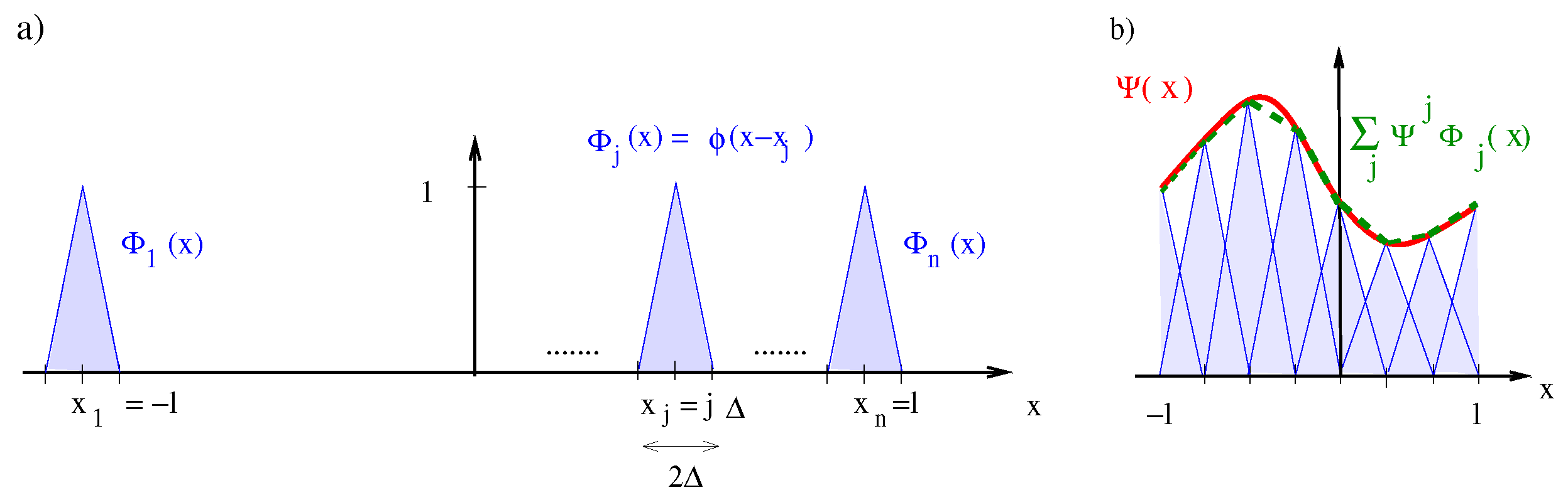
In the finite element method [30] shifted hat functions are used as basis functions [31,32]

$${\Phi }_j\left(x\right)=\varphi (x-x_j)$$

(32)

(see Figure 2), with

$$\varphi \left(x\right)=\left\{\begin{array}{cc}1-{\displaystyle \frac{x}{\Delta }}\hfill & \mathrm{for} 0\le x/\Delta \le 1\hfill \\ 1+{\displaystyle \frac{x}{\Delta }}\hfill & \mathrm{for} -1\le x/\Delta \le 0\hfill \\ 0\hfill & \mathrm{for} |x/\Delta |\ge 1,\hfill \end{array}\right.$$

(33)

where node point $x_j=-l+(j-1)\Delta$, and $\Delta =2l/(n-1)$. In the particular finite element representation one has in Equations (23) and (24) the relationships ${\Phi }_j(-l)={\delta }_{j,1}$ and ${\Phi }_j\left(l\right)={\delta }_{j,n}$. Then in Section 3 the R-matrix (25) in weak formulation simplifies to

$$R_{s{s}^{\prime }}={\left({\displaystyle \frac{1}{h-ϵb}}\right)}_{j\left(s\right),j\left(s^{\prime }\right)}$$

(34)

with

$$j\left(s\right)=\left\{\begin{array}{cc}1\hfill & \mathrm{for} s=1\hfill \\ n\hfill & \mathrm{for} s=2.\hfill \end{array}\right.$$

(35)

Inserting (32) in (4) and (5) it turns out that h and b are real, symmetric tridiagonal matrices. In particular we use

$$I_1={\int }_{-\Delta }^{\Delta }dx\varphi {\left(x\right)}^2=2{\int }_0^{\Delta }dx{\left(1-{\displaystyle \frac{x}{\Delta }}\right)}^2={\displaystyle \frac{2\Delta }{3}}$$

(36)

and thus

$$b_{jj}=I_1\left(1-{\displaystyle \frac{{\delta }_{j,1}+{\delta }_{j,n}}{2}}\right).$$

(37)

With

$$\begin{array}{ccc}\hfill I_2& =& {\int }_{-\Delta }^{\Delta }dx\varphi \left(x\right)\varphi (x-\Delta )={\int }_0^{\Delta }dx\left(1-{\displaystyle \frac{x}{\Delta }}\right){\displaystyle \frac{x}{\Delta }}={\displaystyle \frac{\Delta }{6}}.\hfill \end{array}$$

(38)

one finds

$$b_{j{j}^{\prime }}=\left\{\begin{array}{cc}{I}_1\left(1-{\displaystyle \frac{{\delta }_{j,1}+{\delta }_{j,n}}{2}}\right)\hfill & \mathrm{for} j=j^{\prime }\hfill \\ I_2\hfill & \mathrm{for} |j-j^{\prime }|=1\hfill \\ 0\hfill & \mathrm{else}.\hfill \end{array}\right.$$

(39)

Furthermore

$$I_3={\int }_{-\Delta }^{\Delta }dx{\varphi }^{\prime }{\left(x\right)}^2=2{\int }_0^{\Delta }dx{\left({\displaystyle \frac{1}{\Delta }}\right)}^2={\displaystyle \frac{2}{\Delta }}$$

(40)

and

$$\begin{array}{ccc}\hfill I_4& =& {\int }_{-\Delta }^{\Delta }dx{\varphi }^{\prime }\left(x\right){\varphi }^{\prime }(x-\Delta )={\int }_0^{\Delta }dx\left(-{\displaystyle \frac{1}{\Delta }}\right){\displaystyle \frac{1}{\Delta }}={\displaystyle \frac{\Delta }{6}}.\hfill \end{array}$$

(41)

Then

$$h_{j{j}^{\prime }}=\left\{\begin{array}{cc}{I}_3\left(1-{\displaystyle \frac{{\delta }_{j,1}+{\delta }_{j,n}}{2}}\right)+v_{j{j}^{\prime }}\hfill & \mathrm{for} j=j^{\prime }\hfill \\ I_4+v_{j{j}^{\prime }}\hfill & \mathrm{for} |j-j^{\prime }|=1\hfill \\ 0\hfill & \mathrm{else}\hfill \end{array}\right.$$

(42)

with

$$v_{j{j}^{\prime }}={\int }_{-l}^{l}dx\varphi (x-x_j)v\left(x\right)\varphi (x-x_{j^{\prime }}).$$

(43)

For the finite element basis, the set of inhomogeneous linear equations Equation (A7) in Appendix A is furthermore reduced on the right side by

$${\left(c\right)}_{j{j}^{\prime }}=i{k}_2{\delta }_{j,n}{\delta }_{j^{\prime },n}+i{k}_1{\delta }_{j,1}{\delta }_{j^{\prime },1}$$

(44)

and on the left side one has for the inhomogeneity $-2i{k}_1{\Phi }_j(-l)=-2i{k}_1{\delta }_{j,1}$.

Figure 2. (a) The shifted hat functions $\varphi (x-x_j)$ as basis functions ${\Phi }_j\left(x\right)$ in the finite element approximation. (b) Piecewise linear approximation ${\sum }_j{\Psi }^j\varphi (x-x_j)$ (green) of the wave function $\Psi \left(x\right)$ (red) in the finite element basis.

Figure 2. (a) The shifted hat functions $\varphi (x-x_j)$ as basis functions ${\Phi }_j\left(x\right)$ in the finite element approximation. (b) Piecewise linear approximation ${\sum }_j{\Psi }^j\varphi (x-x_j)$ (green) of the wave function $\Psi \left(x\right)$ (red) in the finite element basis.

6. Discussion and Conclusions

We have presented the Schrödinger scattering problem in one dimension in weak formulation. Two solution procedures have been discussed: The first procedure is the construction of individual scattering states and transmission coefficients as a unique solution of a set of linear equations (see Appendix A). The second procedure is the R-matrix method in which the S-matrix is constructed via the R-matrix. The S-matrix contains the transmission coefficients of all scattering states at once. Both procedures are not equivalent. In particular, the construction of the S-matrix leads to a current-conserving approximation while construction of individual scattering states in the first procedure does not necessarily lead to a current-conserving approximation. To illustrate this point we study here a simple example with $n=1$ and $V_2=0$ setting $k_1=k_2=k$, and ${\Phi }_1\left(x\right)=\Phi \left(x\right)$.

6.1. Individual Scattering States as Solution of a Set of Linear Equations (‘Direct Calculation’)

In our simple example Equation (A2) becomes

$$ik({\Psi }_2^{out}-{\Psi }_2^{in})\Phi \left(l\right)+ik({\Psi }_1^{out}-{\Psi }_1^{in})\Phi (-l)=\left(h-ϵb\right){\Psi }^1$$

(45)

with $h_{11}\equiv h$, and $b_{11}\equiv b$. Furthermore, Equations (A3) and (A4) yield

$${\Psi }_1^{in}+{\Psi }_1^{out}={\Psi }^1\Phi (-l)$$

(46)

and

$${\Psi }_2^{in}+{\Psi }_2^{out}={\Psi }^1\Phi \left(l\right).$$

(47)

Here we have three linear equations for five unknowns ${\Psi }^1,{\Psi }_1^{in},{\Psi }_1^{out},{\Psi }_2^{in}$, and ${\Psi }_2^{out}$. To specify a unique solution, two of the coefficients can be chosen freely. To construct the scattering states we regard ${\Psi }_1^{in}$ and ${\Psi }_2^{in}$ as known. To eliminate the out-going coefficients, we insert

$${\Psi }_1^{out}={\Psi }^1\Phi (-l)-{\Psi }_1^{in}$$

(48)

$${\Psi }_2^{out}={\Psi }^1\Phi \left(l\right)-{\Psi }_2^{in}.$$

(49)

into (45). Assuming further the source-incident scattering state, ${\Psi }_1^{in}=1$ and ${\Psi }_2^{in}=0$, (45) yields

$$-2ik\Phi (-l)=\left(h-c-ϵb\right){\Psi }^1\Rightarrow {\Psi }^1=-{\displaystyle \frac{2ik\Phi (-l)}{h-c-ϵb}}$$

(50)

with $c_{11}\equiv c$ corresponding to (A7). From (48)

$${\Psi }_1^{out}=S_{11}=r^1=-1+{\Psi }^1\Phi (-l)=-1-{\displaystyle \frac{2ik\Phi {(-l)}^2}{h-c-ϵb}}$$

(51)

corresponding to (A8) and from (49)

$${\Psi }_2^{out}=S_{21}=t^1={\Psi }^1\Phi \left(l\right)=-{\displaystyle \frac{2ik\Phi (-l)\Phi \left(l\right)}{h-c-ϵb}}$$

(52)

corresponding to (A9). For current conservation we require, from (A13),

$$\begin{array}{ccc}& & |S_{11}{|}^2+{|S_{21}|}^2=1+{\displaystyle \frac{4k^2\Phi {(-l)}^4}{{(h-c-ϵb)}^2}}+{\displaystyle \frac{4k^2\Phi {(-l)}^2\Phi {\left(l\right)}^2}{{(h-c-ϵb)}^2}}\stackrel{!}{=}1\hfill \\ & \Rightarrow & {\displaystyle \frac{4k^2}{{(h-c-ϵb)}^2}}\Phi {(-l)}^2\left[\Phi {\left(l\right)}^2+\Phi {(-l)}^2\right]=0.\hfill \end{array}$$

(53)

The latter condition requires total reflection, $\Phi (-l)=0$; i.e., it is generally not fulfilled.

6.2. R-Matrix Method

In our simple example we obtain from (25)

$$R_{s{s}^{\prime }}={\displaystyle \frac{1}{h-ϵb}}\Phi \left[{(-1)}^{s}l\right]\Phi \left[{(-1)}^{s^{\prime }}l\right]$$

(54)

which is of course a bad approximation for the R-matrix in strong formulation. However, our approximation for the R-matrix is real and symmetrical, which is why we nevertheless obtain a current-conserving approximation. From Equation (17) one obtains a real, symmetric current R-matrix

$$\Omega =\left(\begin{array}{cc}{\Omega }_1& {\Omega }_d\\ {\Omega }_d& {\Omega }_2\end{array}\right)$$

(55)

with ${\Omega }_1=k\Phi (-l)\Phi (-l)/(h-ϵb)$, ${\Omega }_2=k\Phi \left(l\right)\Phi \left(l\right)/(h-ϵb)$, and ${\Omega }_D=k\Phi \left(l\right)\Phi (-l)/(h-ϵb)$. With elementary transformations Equation (16) yields

$$\begin{array}{ccc}& & \tilde{S}=S=-{\displaystyle \frac{1+i\Omega }{1-i\Omega }}=-{\displaystyle \frac{1}{1-{\Omega }_1{\Omega }_2+{\Omega }_d^2-i({\Omega }_1+{\Omega }_2)}}\hfill \\ & & \times \left(\begin{array}{cc}1+{\Omega }_1{\Omega }_2-{\Omega }_d^2+i({\Omega }_1-{\Omega }_2)& 2i{\Omega }_d\\ 2i{\Omega }_d& 1+{\Omega }_1{\Omega }_2-{\Omega }_d^2-i({\Omega }_1-{\Omega }_2)\end{array}\right).\hfill \end{array}$$

(56)

One establishes easily the unitarity of $\tilde{S}$ and S; i.e., both column vectors have an absolute value of unity and they are orthogonal to each other. From the unitarity of S one finds, in contrast to (53), current conservation. From the unitary of the first column vector one has

$$|S_{11}{|}^2+{|S_{21}|}^2=1.$$

(57)

Appendix C.1. The Rayleigh Quotient

Multiplying (A17) by $\chi$ one obtains after partial integration in the interval $⟨-l,l⟩$

$$\begin{array}{ccc}& & {\int }_{-l}^{l}dx[{{\chi }^{\prime }}^2+v{\chi }^2]+\chi (-l){\chi }^{\prime }(-l)-\chi \left(l\right){\chi }^{\prime }\left(l\right)=ϵ{\int }_{-l}^{l}dx{\chi }^2\hfill \\ & \iff & {\int }_{-l}^{l}dx[{{\chi }^{\prime }}^2+v{\chi }^2]+\alpha \left[\chi {(-l)}^2+\chi {\left(l\right)}^2\right]=ϵ{\int }_{-l}^{l}dx{\chi }^2.\hfill \end{array}$$

(A19)

One defines the Rayleigh quotient

$$\mathcal{R}\left(\chi \right)\equiv {\displaystyle \frac{{\int }_{-l}^{l}dx[{{\chi }^{\prime }}^2+v{\chi }^2]+\alpha \left[\chi {(-l)}^2+\chi {\left(l\right)}^2\right]}{{\int }_{-l}^{l}dx{\chi }^2}}\equiv {\displaystyle \frac{⟨\chi |\widehat{H}|\chi ⟩}{⟨\chi |\chi ⟩}}$$

(A20)

which can be interpreted as the expectation value of the energy operator $\widehat{H}=-{\displaystyle \frac{d^2}{d{x}^2}}+v\left(x\right)$ in the state $|\chi ⟩$.

Since the eigenstates $|{\chi }_i⟩$ in (A17) can be chosen as a complete orthonormal system, for a general state we can write

$$|\chi ⟩=\sum _i{a}_i|{\chi }_i⟩\mathrm{with}{a}_i=⟨{\chi }_i\mid \chi ⟩.$$

(A21)

Insertion of the expansion (A21) in (A20) leads to

$$ϵ={\displaystyle \frac{{\sum }_{i=1}^{\infty }{ϵ}_i{|a_i|}^2}{{\sum }_{i=1}^{\infty }{|a_i|}^2}}\ge {ϵ}_1{\displaystyle \frac{{\sum }_{i=1}^{\infty }{|a_i|}^2}{{\sum }_{i=1}^{\infty }{|a_i|}^2}}={ϵ}_1$$

(A22)

Since $ϵ\ge {ϵ}_1$ for an arbitrary $|\chi ⟩$ the groundstate $|{\chi }_1⟩$ is given by the condition

$${ϵ}_1=Minϵ\left(\chi \right).$$

(A23)

The higher eigenvalues ${ϵ}_{i\ge 2}$, and eigenstates we obtain by successive reduction of the considered subspaces to orthogonal complements of all the already found eigenstates and applying the above minimization procedure in the subspaces.

Appendix C.2. Ritz Method: Space Restricted to Linear Combinations of Atomic Orbitals (LCAOs)

Inserting in the LCAO expansion (28) in (A20) the Rayleigh–Ritz coefficient takes the form

$$\mathcal{R}(u_1,\dots ,u_n)={\displaystyle \frac{{\sum }_{j=1}^n{\sum }_{j^{\prime }=1}^n{u}^j{u}^{j^{\prime }}{h}_{j{j}^{\prime }}+\alpha a_{j{j}^{\prime }}}{{\sum }_{j=1}^n{\sum }_{j^{\prime }=1}^n{u}^j{u}^{j^{\prime }}{b}_{j{j}^{\prime }}}}={\displaystyle \frac{⟨\Psi |\widehat{H}|\Psi ⟩}{⟨\Psi |\Psi ⟩}}$$

(A24)

with the further matrix

$$a_{j{j}^{\prime }}={\Phi }_j(-l){\Phi }_{j^{\prime }}(-l)+{\Phi }_j\left(l\right){\Phi }_{j^{\prime }}\left(l\right).$$

(A25)

The extremes of $ϵ$ are determined by the conditions $\partial ϵ/(\partial u^j)=0$. We find

$${\displaystyle \frac{\partial ϵ}{\partial u^j}}={\displaystyle \frac{1}{⟨\chi \mid \chi ⟩}}\left[{\displaystyle \frac{\partial }{\partial u^j}}⟨\chi |\widehat{H}|\chi ⟩-\underset{ϵ}{\underbrace{{\displaystyle \frac{⟨\chi |\widehat{H}|\chi ⟩}{⟨\chi \mid \chi ⟩}}}}{\displaystyle \frac{\partial }{\partial u^j}}⟨\chi \mid \chi ⟩\right]\stackrel{!}{=}0.$$

(A26)

from which follows

$${\displaystyle \frac{\partial }{\partial u^j}}⟨\chi |\widehat{H}|\chi ⟩-ϵ{\displaystyle \frac{\partial }{\partial u^j}}⟨\chi \mid \chi ⟩=0.$$

(A27)

In the latter equation we have

$${\displaystyle \frac{\partial }{\partial u^j}}⟨\chi |\widehat{H}|\chi ⟩={\displaystyle \frac{\partial }{\partial u^j}}\left[\sum _{j^{\prime },j^{\prime \prime }=1}^n{u}^{j^{\prime }}{u}^{j^{\prime \prime }}\left(h_{j^{\prime }{j}^{\prime \prime }}+\alpha a_{j^{\prime }{j}^{\prime \prime }}\right)\right]=2\sum _{j^{\prime }=1}^n\left(h_{j{j}^{\prime }}+\alpha a_{j{j}^{\prime }}\right)u^{j^{\prime }}$$

(A28)

and

$${\displaystyle \frac{\partial }{\partial u^j}}⟨\chi \mid \chi ⟩={\displaystyle \frac{\partial }{\partial u^j}}\left(\sum _{j^{\prime }=1}^n\sum _{j^{\prime \prime }=1}^n{u}^{j^{\prime }}{u}^{j^{\prime \prime }}{b}_{j^{\prime }{j}^{\prime \prime }}\right)=2\sum _{j^{\prime }=1}^n{b}_{j{j}^{\prime }}{u}^{j^{\prime }}.$$

(A29)

Insertion in (A27) leads to the best LCAO approximation for the Wigner–Eisenbud functions and -energies which is determined by the equation

$$\sum _{j^{\prime }=1}^n(h_{j{j}^{\prime }}+\alpha a_{j{j}^{\prime }}-{ϵ}_i{b}_{j{j}^{\prime }})u_i^{j^{\prime }}=0.$$

(A30)

Since h, a and b are real symmetric matrices it follows that one obtains n real eigenvalues ${ϵ}_i$ and the expansion coefficients $u_i^j$ can be chosen as real. For $\alpha =0$ this equation reduces to (20). It follows that the ${\chi }_i$ and ${ϵ}_i$ are in fact the best LCAO approximation for the Wigner–Eisenbud functions and energies for $\alpha =0$.

References

- Frenkel, J. On the Electrical Resistance of Contacts between Solid Conductors. Phys. Rev. 1930, 36, 1604. [Google Scholar] [CrossRef] [Scilit]
- Ehrenberg, W.; Hönl, H. Zur Theorie des elektrischen Kontaktes. Z. Phys. 1931, 68, 289. [Google Scholar] [CrossRef] [Scilit]
- Landauer, R. Spatial variation of currents and fields due to localized scatterers in metallic conduction. IBM J. Res. Develop. 1957, 1, 223. [Google Scholar] [CrossRef] [Scilit]
- Landauer, R. Electrical transport in open and closed systems. Z. Phys. B 1987, 68, 217. [Google Scholar] [CrossRef] [Scilit]
- Tsu, R.; Esaki, L. Tunneling in a finite superlattice. Appl. Phys. Lett. 1973, 22, 562. [Google Scholar] [CrossRef] [Scilit]
- Fisher, D.S.; Lee, P.A. Relation between conductivity and transmission matrix. Phys. Rev. B 1981, 23, 6851. [Google Scholar] [CrossRef] [Scilit]
- Büttiker, M.; Imry, Y.; Landauer, R.; Pinhas, S. Generalized many-channel conductance formula with application to small rings. Phys. Rev. B 1985, 31, 6207. [Google Scholar] [CrossRef] [Scilit]
- Büttiker, M. Four-Terminal Phase-Coherent Conductance. Phys. Rev. Lett. 1986, 57, 1761. [Google Scholar] [CrossRef] [Scilit] [PubMed]
- Büttiker, M. Symmetry of electrical conduction. IBM J. Res. Dev. 1988, 32, 317. [Google Scholar] [CrossRef] [Scilit]
- Wulf, U.; Kučera, J.; Richter, H.; Horstmann, M.; Wiatr, M.; Höntschel, J. Channel engineering for nanotransistors in a semiempirical quantum transport model. Mathematics 2017, 5, 68. [Google Scholar] [CrossRef] [Scilit]
- Nemnes, G.A.; Ion, L.; Antohe, S. Self-consistent potentials and linear regime conductance of cylindrical nanowire transistors in the R-matrix formalism. J. Appl. Phys. 2009, 106, 113714. [Google Scholar] [CrossRef] [Scilit]
- Nemnes, G.A.; Manolescu, A.; Gudmundsson, V. Reduction of ballistic spin scattering in a spin-FET using stray electric fields. J. Physics Conf. Ser. 2012, 338, 012012. [Google Scholar] [CrossRef] [Scilit]
- Nemnes, G.A.; Dragoman, D. Reconfigurable quantum logic gates using Rashba controlled spin polarized currents. Phys. E 2019, 111, 13. [Google Scholar] [CrossRef] [Scilit]
- Wulf, U. An Electron Waveguide Model for FDSOI Transistors. Solids 2022, 3, 203–218. [Google Scholar] [CrossRef] [Scilit]
- Wulf, U.; Preda, A.T.; Nemnes, G.A. Transport in a Two-Channel Nanotransistor Device with Lateral Resonant Tunneling. Micromachines 2024, 15, 1270. [Google Scholar] [CrossRef] [Scilit] [PubMed]
- Lane, A.M.; Thomas, R.G. R-Matrix Theory of Nuclear Reactions. Rev. Mod. Phys. 1958, 30, 257. [Google Scholar] [CrossRef] [Scilit]
- Burke, P.G.; Berrington, K.A. (Eds.) Atomic and Molecular Processes: An R-Matrix Approach; Institute of Physics Publishing: Bristol, UK, 1993. [Google Scholar]
- Kapur, P.L.; Peierls, R. The dispersion formula for nuclear reactions. Proc. R. Soc. Lond. 1938, A166, 277. [Google Scholar] [CrossRef] [Scilit]
- Smrčka, L. R-matrix and the coherent transport in mesoscopic systems. Superlattices Microstruct. 1990, 8, 221. [Google Scholar] [CrossRef] [Scilit]
- Rektorys, K. Variational Methods in Mathematics, Science and Engineering; D. Reidel: Dordrecht, The Netherlands, 1977. [Google Scholar] [CrossRef] [Scilit]
- Kirkner, D.; Lent, C. The quantum transmitting boundary method. J. Appl. Phys. 1990, 67, 6353. [Google Scholar] [CrossRef] [Scilit]
- Leng, M.; Lent, C.S. Recovery of quantized ballistic conductance in a periodically modulated channel. Phys. Rev. Lett. 1993, 71, 137. [Google Scholar] [CrossRef] [Scilit]
- Leng, M.; Lent, C.S. Quantum transmitting boundary method in a magnetic field. J. Appl. Phys. 1994, 76, 2240. [Google Scholar] [CrossRef] [Scilit]
- Leng, M.; Lent, C.S. Conductance quantization in a periodically modulated channel. Phys. Rev. B 1994, 50, 10823. [Google Scholar] [CrossRef] [Scilit]
- Shao, Z.; Porod, W.; Lent, C.S.; Kirkner, D.J. An eigenvalue method for open-boundary quantum transmission problems. J. Appl. Phys. 1995, 78, 2177. [Google Scholar] [CrossRef] [Scilit]
- Kučera, J.; Wulf, U. Scattering Theory in an N-pole semiconductor quantum device: Unitarity of the current S-matrix and current conservation. Micromachines 2025, 16, 306. [Google Scholar] [CrossRef] [Scilit] [PubMed]
- Cayley, A. Sur quelques proprietes des determinants gauches. J. Die Reine Angew. Math. 1846, 32, 119. [Google Scholar] [CrossRef] [Scilit]
- Mondal, S.; Sivakumar, K.; Tsatsomeros, M. The Cayley transform of prevalent matrix classes. Linear Algebra Its Appl. 2024, 681, 1. [Google Scholar] [CrossRef] [Scilit]
- Wulf, U. A One-Dimensional Effective Model for Nanotransistors in Landauer-Büttiker Formalism. Micromachines 2020, 11, 359. [Google Scholar] [CrossRef] [Scilit]
- Morton, K.W. Basic course in finite element methods. Comput. Phys. Rep. 1987, 6, 1–72. [Google Scholar] [CrossRef] [Scilit]
- Hughes, T.J.R. Piecewise Linear Finite Element Space. In The Finite Element Method: Linear Static and Dynamic Finite Element Analysis; Courier Corporation: North Chelmsford, MA, USA, 2012; p. 20. [Google Scholar]
- Velte, W. Die Methode der finiten Elemente. In Direkte Methoden der Variationsrechnung; B. G. Teubner: Stuttgart, Germany, 1976; p. 82. [Google Scholar] [CrossRef] [Scilit]
- Zwillinger, D. Sturm-Liouville Theory. In Handbook of Differential Equations, 2nd ed.; Academic Press, Inc.: San Diego, CA, USA, 1992; p. 82. [Google Scholar] [CrossRef] [Scilit]
Disclaimer/Publisher’s Note: The statements, opinions and data contained in all publications are solely those of the individual author(s) and contributor(s) and not of MDPI and/or the editor(s). MDPI and/or the editor(s) disclaim responsibility for any injury to people or property resulting from any ideas, methods, instructions or products referred to in the content. |
© 2025 by the authors. Licensee MDPI, Basel, Switzerland. This article is an open access article distributed under the terms and conditions of the Creative Commons Attribution (CC BY) license (https://creativecommons.org/licenses/by/4.0/).