
Energy-Gap-Refractive Index Relations in Semiconductors—Using Wemple–DiDomenico Model to Unify Moss, Ravindra, and Herve–Vandamme Relationships


Abstract
:1. Introduction
2. Mathematical Formulation
3. , , and
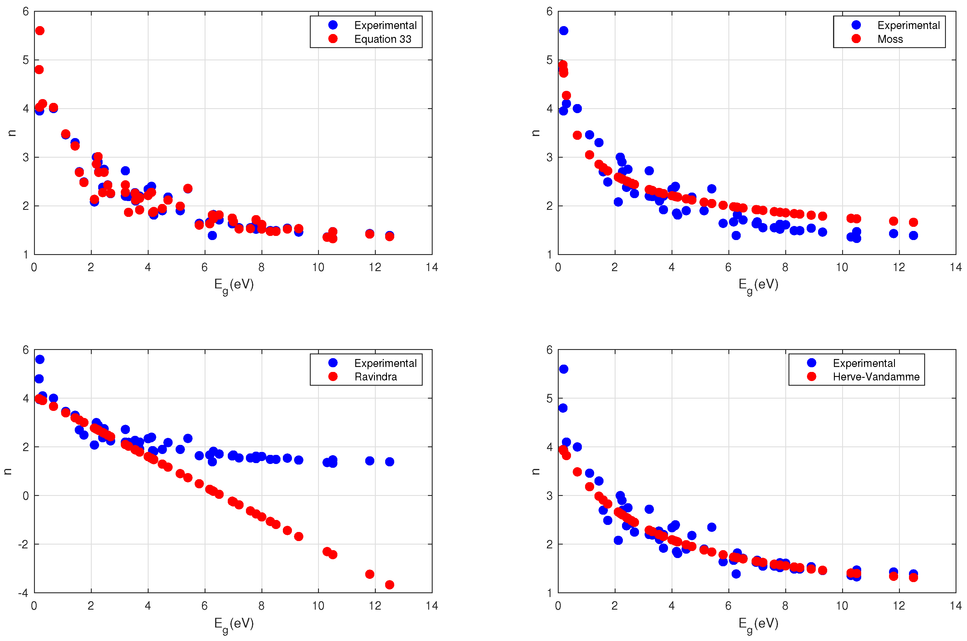
4. Results
4.1. Moss Relation
4.2. Ravindra Relation
4.3. Herve–Vandamme Relation
5. Discussion
5.1. Empirical Fitting Constants
5.2. Convergence Criterion
5.3. Exceptional Materials
6. Conclusions
Funding
Data Availability Statement
Acknowledgments
Conflicts of Interest
References
- Ou, Q.; Bao, X.; Zhang, Y.; Shao, H.; Xing, G.; Li, X.; Shao, L.; Bao, Q. Band structure engineering in metal halide perovskite nanostructures for optoelectronic applications. Nano Mater. Sci. 2019, 1, 268–287. [Google Scholar] [CrossRef]
- Geng, T.; Ma, Z.; Chen, Y.; Cao, Y.; Lv, P.; Li, N.; Xiao, G. Bandgap engineering in two-dimensional halide perovskite Cs 3 Sb 2 I 9 nanocrystals under pressure. Nanoscale 2020, 12, 1425–1431. [Google Scholar] [CrossRef]
- Wu, M.J.; Kuo, C.C.; Jhuang, L.S.; Chen, P.H.; Lai, Y.F.; Chen, F.C. Bandgap engineering enhances the performance of mixed-cation perovskite materials for indoor photovoltaic applications. Adv. Energy Mater. 2019, 9, 1901863. [Google Scholar] [CrossRef]
- Nenkov, M.R.; Pencheva, T.G. Determination of thin film refractive index and thickness by means of film phase thickness. Cent. Eur. J. Phys. 2008, 6, 332–343. [Google Scholar] [CrossRef]
- Ono, M.; Aoyama, S.; Fujinami, M.; Ito, S. Significant suppression of Rayleigh scattering loss in silica glass formed by the compression of its melted phase. Opt. Express 2018, 26, 7942–7948. [Google Scholar] [CrossRef]
- Ong, H.; Dai, J.; Li, A.; Du, G.; Chang, R.; Ho, S. Effect of a microstructure on the formation of self-assembled laser cavities in polycrystalline ZnO. J. Appl. Phys. 2001, 90, 1663–1665. [Google Scholar] [CrossRef]
- Moss, T.S. A Relationship between the Refractive Index and the Infra-Red Threshold of Sensitivity for Photoconductors. Proc. Phys. Soc. Sect. B 1950, 63, 167. [Google Scholar] [CrossRef]
- Moss, T.S. Photoconductivity in the Elements. Proc. Phys. Soc. Sect. A 1951, 64, 590. [Google Scholar] [CrossRef]
- Ravindra, N.; Srivastava, V. Variation of refractive index with energy gap in semiconductors. Infrared Phys. 1979, 19, 603–604. [Google Scholar] [CrossRef]
- Reddy, R.; Nazeer Ahammed, Y. A study on the Moss relation. Infrared Phys. Technol. 1995, 36, 825–830. [Google Scholar] [CrossRef]
- Ravindra, N.; Auluck, S.; Srivastava, V. On the Penn Gap in Semiconductors. Phys. Status Solidi (b) 1979, 93, K155–K160. [Google Scholar] [CrossRef]
- Gupta, V.; Ravindra, N. Comments on the Moss Formula. Phys. Status Solidi (b) 1980, 100, 715–719. [Google Scholar] [CrossRef]
- Penn, D.R. Wave-Number-Dependent Dielectric Function of Semiconductors. Phys. Rev. 1962, 128, 2093–2097. [Google Scholar] [CrossRef]
- Wemple, S.; DiDomenico, M., Jr. Behavior of the electronic dielectric constant in covalent and ionic materials. Phys. Rev. B 1971, 3, 1338. [Google Scholar] [CrossRef]
- Wemple, S.H.; DiDomenico, M. Optical Dispersion and the Structure of Solids. Phys. Rev. Lett. 1969, 23, 1156–1160. [Google Scholar] [CrossRef]
- Hervé, P.; Vandamme, L. General relation between refractive index and energy gap in semiconductors. Infrared Phys. Technol. 1994, 35, 609–615. [Google Scholar] [CrossRef]
- Finkenrath, H. The Moss rule and the influence of doping on the optical dielectric constant of semiconductors—I. Infrared Phys. 1988, 28, 327–332. [Google Scholar] [CrossRef]
- Sellmeier. Zur Erklärung der abnormen Farbenfolge im Spectrum einiger Substanzen. Ann. Der Phys. 1871, 219, 272–282. [Google Scholar] [CrossRef]
- Levi, A.F.J. The Lorentz oscillator model. In Essential Classical Mechanics for Device Physics; Morgan & Claypool Publishers: San Rafael, CA, USA, 2016; pp. 5-1–5-21, 2053–2571. [Google Scholar] [CrossRef]
- Gomaa, H.M.; Yahia, I.; Zahran, H. Correlation between the static refractive index and the optical bandgap: Review and new empirical approach. Phys. B Condens. Matter 2021, 620, 413246. [Google Scholar] [CrossRef]
- Moss, T.S. Relations between the Refractive Index and Energy Gap of Semiconductors. Phys. Status Solidi (b) 1985, 131, 415–427. [Google Scholar] [CrossRef]
- Ravindra, N.; Ganapathy, P.; Choi, J. Energy gap–refractive index relations in semiconductors—An overview. Infrared Phys. Technol. 2007, 50, 21–29. [Google Scholar] [CrossRef]

| Ravindra Constants: ; | H-V Constants: A; B | Moss Constant | |||||
|---|---|---|---|---|---|---|---|
| C | 5.4 | 10.9 | 49.7 | 3.32; 0.30 | 23.27; 5.5 | 166.91 | 2.35 |
| 1.1 | 4.0 | 44.4 | 4.08; 0.70 | 13.32; 2.9 | 161.06 | 3.46 | |
| 0.67 | 2.7 | 41.0 | 4.64; 1.14 | 10.52; 2.03 | 175.51 | 4.0 | |
| 1.43 | 3.55 | 33.5 | 4.18; 0.98 | 10.90; 2.12 | 155.76 | 3.3 | |
| 2.24 | 4.46 | 36.0 | 4.27; 0.96 | 12.67; 2.22 | 184.34 | 2.9 | |
| 0.18 | 2.3 | 35.0 | 4.19; 0.99 | 8.97; 2.12 | 47.34 | 3.95 | |
| 2.45 | 5.6 | 34.9 | 3.58; 0.57 | 13.98; 3.15 | 128.14 | 2.75 | |
| 2.18 | 4.7 | 33.7 | 3.90; 0.77 | 12.58; 2.52 | 145.52 | 3.0 | |
| 12.50 | 17.1 | 14.9 | 2.63; 0.28 | 15.96; 4.6 | 43.77 | 1.39 | |
| 10.5 | 15 | 11.3 | 2.42; 0.27 | 13.01; 4.5 | 32.28 | 1.33 | |
| 10.3 | 14.8 | 12.3 | 2.45; 0.27 | 13.50; 4.5 | 34.53 | 1.36 | |
| 8.9 | 10.3 | 13.6 | 4.13; 1.47 | 11.83; 1.40 | 47.92 | 1.54 | |
| 8.5 | 10.5 | 12.3 | 3.38; 0.84 | 11.96; 2 | 40.08 | 1.49 | |
| 8.3 | 10.4 | 12.2 | 3.28; 0.78 | 11.26; 2.1 | 39.19 | 1.49 | |
| 8 | 10.6 | 14 | 3.97; 0.59 | 12.18; 2.60 | 43.09 | 1.61 | |
| 7.6 | 9.2 | 12.4 | 3.67; 1.15 | 10.68; 1.60 | 41.90 | 1.55 | |
| 7.2 | 9.1 | 12.1 | 3.34; 0.88 | 10.54; 1.90 | 39.08 | 1.55 | |
| 6.17 | 7.7 | 12.8 | 3.66; 1.19 | 9.92; 1.53 | 43.73 | 1.67 | |
| 5.8 | 7.7 | 12.1 | 3.23; 0.85 | 9.65; 1.90 | 38.35 | 1.64 | |
| 8.0 | 10.6 | 17.1 | 3.26; 0.63 | 13.46; 2.6 | 54.63 | 1.61 | |
| 7.0 | 9.4 | 17 | 3.32; 0.69 | 12.64; 2.40 | 55.21 | 1.67 | |
| 6.3 | 7.5 | 15.2 | 4.35; 1.81 | 10.67; 1.20 | 57.71 | 1.82 | |
| 2.11 | 5.8 | 20.6 | 2.67; 0.36 | 10.93; 3.69 | 43.71 | 2.08 | |
| 2.68 | 5.3 | 21.7 | 3.21; 0.61 | 10.72; 2.62 | 69.55 | 2.25 | |
| 11.8 | 15.7 | 15.9 | 2.84; 0.36 | 15.80; 3.90 | 47.80 | 1.43 | |
| 10.5 | 13.8 | 15.9 | 3.0; 0.45 | 14.81; 3.3 | 48.63 | 1.47 | |
| 5.13 | 7.4 | 22 | 3.6; 0.80 | 12.76; 2.27 | 80.97 | 1.9 | |
| 3.31 | 7.3 | 18.1 | 2.52; 0.31 | 11.49; 3.99 | 40.07 | 2.19 | |
| 3.7 | 6.4 | 17.1 | 2.95; 0.55 | 10.46; 2.70 | 49.88 | 1.92 | |
| 2.4 | 4.9 | 20.4 | 3.18; 0.64 | 9.99; 2.5 | 63.98 | 2.38 | |
| 1.74 | 4.0 | 20.6 | 3.29; 0.73 | 9.08; 2.26 | 65.81 | 2.49 | |
| 3.54 | 6.15 | 25.2 | 3.46; 0.66 | 12.45; 2.61 | 91.98 | 2.27 | |
| 7.8 | 11.3 | 22.0 | 3.08; 0.44 | 15.77; 3.5 | 67.74 | 1.62 | |
| 6.26 | 9.9 | 22.6 | 2.98; 0.41 | 14.96; 3.64 | 67.46 | 1.39 | |
| 6.96 | 13.4 | 27.5 | 2.52; 0.195 | 19.19; 6.44 | 64.84 | 1.63 | |
| 6.5 | 11.1 | 25.4 | 2.82; 0.31 | 16.80; 4.60 | 70.28 | 1.71 | |
| 3.7 | 6.24 | 23.2 | 3.40; 0.67 | 12.03; 2.54 | 82.36 | 2.2 | |
| 4.10 | 5.68 | 23.7 | 4.31; 1.36 | 11.60; 1.58 | 109.70 | 2.38 | |
| 4.12 | 5.57 | 23.3 | 4.46; 1.54 | 11.40; 1.45 | 110.68 | 2.4 | |
| 3.70 | 6.50 | 23.7 | 3.28; 0.58 | 12.41; 2.8 | 79.87 | 2.2 | |
| 4.7 | 7.49 | 26.1 | 3.47; 0.62 | 13.98; 2.80 | 94.53 | 2.18 | |
| 4.0 | 6.65 | 25.9 | 3.50; 0.66 | 13.12; 2.65 | 95.83 | 2.34 | |
| 3.2 | 5.24 | 25.7 | 3.89; 0.95 | 11.60; 2.04 | 111.56 | 2.72 | |
| 7.80 | 12.1 | 23.3 | 2.87; 0.33 | 16.80; 4.3 | 66.76 | 1.52 | |
| 4.20 | 9.15 | 23.3 | 2.56; 0.25 | 14.60; 4.95 | 52.82 | 1.81 | |
| 3.56 | 7.46 | 26.0 | 2.93; 0.37 | 13.93; 3.9 | 71.62 | 2.1 | |
| 4.50 | 8.26 | 23.0 | 2.88; 0.38 | 13.78; 3.76 | 64.45 | 1.90 | |
| 3.2 | 5.40 | 22.60 | 3.56; 0.81 | 11.04; 2.2 | 86.03 | 2.2 | |
| 4.16 | 8.60 | 21.30 | 2.60; 0.29 | 13.53; 4.44 | 50.28 | 1.85 | |
| 9.3 | 13.6 | 18.3 | 2.72; 0.32 | 15.77; 4.30 | 51.16 | 1.46 | |
| 3.54 | 6.36 | 26.1 | 3.39; 0.60 | 12.88; 2.82 | 92.21 | 2.27 | |
| 2.58 | 5.54 | 27.0 | 3.31; 0.56 | 12.23; 2.96 | 89.0 | 2.43 | |
| 2.26 | 4.34 | 27.0 | 3.88; 0.93 | 10.82; 2.08 | 117.85 | 2.70 | |
| 1.58 | 4.13 | 25.7 | 3.42; 0.67 | 10.30; 2.55 | 82.42 | 2.7 | |
| 0.286 | 3.5 | 55.33 | 4.28; 0.66 | 13.91; 3.21 | 80.55 | 4.1 | |
| 0.165 | 3.0 | 66.12 | 4.94; 0.87 | 14.08; 2.83 | 87.58 | 4.8 | |
| 0.190 | 2.2 | 66.80 | 5.86; 1.46 | 12.12; 2.01 | 186.90 | 5.6 |
| Moss (n) | Ravindra (n) | H-V (n) | Equation (33) (n) | |||
|---|---|---|---|---|---|---|
| 0.67 | 3.45 | 3.66 | 3.48 | 4.02 | 4.0 | |
| 0.18 | 4.79 | 3.97 | 3.93 | 4.02 | 3.95 | |
| 0.286 | 4.27 | 3.90 | 3.94 | 4.09 | 4.1 | |
| 0.165 | 4.89 | 3.98 | 3.94 | 4.79 | 4.8 | |
| 0.190 | 4.73 | 3.96 | 3.92 | 5.51 | 5.6 |
Disclaimer/Publisher’s Note: The statements, opinions and data contained in all publications are solely those of the individual author(s) and contributor(s) and not of MDPI and/or the editor(s). MDPI and/or the editor(s) disclaim responsibility for any injury to people or property resulting from any ideas, methods, instructions or products referred to in the content. |
© 2023 by the author. Licensee MDPI, Basel, Switzerland. This article is an open access article distributed under the terms and conditions of the Creative Commons Attribution (CC BY) license (https://creativecommons.org/licenses/by/4.0/).
Share and Cite
Lamichhane, A. Energy-Gap-Refractive Index Relations in Semiconductors—Using Wemple–DiDomenico Model to Unify Moss, Ravindra, and Herve–Vandamme Relationships. Solids 2023, 4, 316-326. https://doi.org/10.3390/solids4040020
Lamichhane A. Energy-Gap-Refractive Index Relations in Semiconductors—Using Wemple–DiDomenico Model to Unify Moss, Ravindra, and Herve–Vandamme Relationships. Solids. 2023; 4(4):316-326. https://doi.org/10.3390/solids4040020
Chicago/Turabian StyleLamichhane, Aneer. 2023. "Energy-Gap-Refractive Index Relations in Semiconductors—Using Wemple–DiDomenico Model to Unify Moss, Ravindra, and Herve–Vandamme Relationships" Solids 4, no. 4: 316-326. https://doi.org/10.3390/solids4040020
APA StyleLamichhane, A. (2023). Energy-Gap-Refractive Index Relations in Semiconductors—Using Wemple–DiDomenico Model to Unify Moss, Ravindra, and Herve–Vandamme Relationships. Solids, 4(4), 316-326. https://doi.org/10.3390/solids4040020