Abstract
Predicting and analyzing the stability of underground stopes is critical for ensuring worker safety, reducing dilution, and maintaining operational efficiency in mining. Traditional stability graphs are widely used but often criticized for oversimplifying the stability phenomenon and relying on subjective classifications. Additionally, the imbalanced nature of stope stability datasets poses challenges for traditional machine learning and statistical models, which often bias predictions toward the majority class. This study proposes a novel methodology for developing site-specific stability graphs using probabilistic modeling and machine learning techniques, addressing the limitations of traditional graphs and the challenges of imbalanced datasets. The approach includes rebalancing of the dataset using the Synthetic Minority Over-Sampling Technique (SMOTE) and feature selection using permutation importance to identify key features that impact instability, using those to construct a bi-dimensional stability graph that provides both improved performance and interpretability. The results indicate that the proposed graph outperforms traditional stability graphs, particularly in identifying unstable stopes, even under highly imbalanced data conditions, highlighting the importance of operational and geometric variables in stope stability, providing actionable insights for mine planners. Conclusively, this study demonstrates the potential for integrating modern probabilistic techniques into mining geotechnics, paving the way for more accurate and adaptive stability assessment tools. Future work includes extending the methodology to multi-mine datasets and exploring dynamic stability graph frameworks.
1. Introduction
Predicting and analyzing the stability of underground rock excavations have been a long-time challenge in the field of geotechnical studies. In particular, for enterprises in the mineral industry that use open stoping methods, an adequate evaluation of stope stability is fundamental to preserve worker safety, reduce the impact of phenomena such as dilution, and ensure the continuity of operations in production galleries.
Studies aiming to evaluate the stability of stopes in mining date back to the 1980s, with the development of the first stability graphs by Mathews et al. [1], later improved by Potvin [2]. Popular in the industry to this day, these early graphs made use of modified values from the rock mass classification system proposed by Barton et al. [3], in correlation with the hydraulic radius of the hangingwall surface to define zones of stability and instability. The premises defined by Mathews and Potvin led to the development of several works associated with stability graphs, such as those produced by Laubscher [4], Villaescusa [5], and Clark [6], the latter introducing the concept of ELOS, with prominent use in the mining industry.
A recurring criticism associated with the graphs, however, is the excessive simplification of the instability phenomenon, where it is reduced to only a few variables when, in practice, it proves to be highly complex. Additionally, there is the implicit subjectivity in the definitions of ‘stable’ and ‘unstable’ within the graphs [7,8]. As such, new lines of study have emerged over the years proposing to investigate stope instability or its consequences, such as dilution, in different ways using various variables. These include multivariate regression [9], computational modeling [10], and logistic regression [11]. More recent research has focused on statistical models and machine learning, such as the work by Qi et al. [12], which used classification through random forests to determine whether a stope is stable or unstable.
In some of the works that use a statistical approach, a noticeable characteristic is the adoption of balanced datasets, that is, datasets where the ratio between the number of ‘stable’ and ‘unstable’ stope observations is less than 1.5 [13]. However, because the mining industry is composed mostly of enterprises aiming for profit, it is expected that mines will trend to have their stopes planned to be stable, making the available datasets either imbalanced or highly imbalanced (when the ratio between the number of ‘stable’ and ‘unstable’ stope observations is greater than 9). In the study performed by Clark [6], about 34 stopes of 47 can be considered stable, making it an imbalanced dataset; in Wang [7], over 60% of the stopes can also be assumed as stable; and even considering Potvin [2]’s stability graph, around 70% of the stopes fell into the stability zone, reinforcing the general notion of imbalance when dealing with stope datasets.
Imbalanced datasets tend to adversely affect the performance of statistical and machine learning models by biasing them towards the majority class [14] and amplifying the effects of issues associated with data, such as a lack of representativity, high dimensionality, and unwanted noise [15]. For that reason, having a methodology that also considers imbalanced datasets is fundamental in order to cover a wider range of mining scenarios.
Considering the aforementioned aspects, this project aims to propose a new methodology to predict the stability of underground stopes by building a dataset composed of field data that characterizes mined stopes, rebalancing the data using a rebalancing algorithm, using that data to estimate the parameters of different probabilistic classifiers, comparing the performance of the models across specific metrics, selecting the two most relevant features, and using those features for the estimation of a bi-dimensional decision frontier that separates the stable and unstable zones.
2. Literature Review
2.1. Stability Graphs
Empirical diagrams for evaluating stope stability have been popular in the mining industry since their introduction in 1980 by Mathews et al. [1], one of the precursors of such studies. The stability graph method was developed with the objective of predicting the stability of open stopes with a steep dip and rock quality ranging from average to good in deep North American mines (above 1000 m deep), initially using a limited case study database [16]. Since the method’s inception, several studies have focused on augmenting the graph with new data from different mines in different contexts. The modifications are associated with changes in the positions of the stability zones and changes in the calculation of factors involved, aiming to extend the applicability of the method for a larger number of mines [17].
The original graph proposed by Mathews had three distinct stability zones separated by transition regions. Potvin [2] modified the graph, reducing the number of zones to two (a stable zone and an unstable zone) separated by a transition. Potvin inserted additional case studies (242 cases, 176 without support and 66 supported), modified the way the joint factor was calculated, and extended the graph to consider supported cases. This variant of the stability graph is known as the modified stability graph. Subsequently, the graph modified by Potvin was further altered by Nickson [18], who inserted an additional 59 cases (14 supported and 45 unsupported), and by Hadjigeorgiou et al. [19], who included more cases (38 supported and 52 unsupported) [6].
The method, however, is often subject to criticism due to its use of qualitative terms to describe the stability zones (“stable” and “unstable”), which makes it difficult to evaluate dilution quantitatively, and due to the lack of consideration for important factors that influence dilution, such as operational factors associated with drilling and blasting, as well as the impact of stope width [7]. Different authors also argue about the method’s limitations, such as the low representativeness of the factors used in the calculations, the excessive simplification of the stope geometry, the lack of consideration for the time a stope remains open, poor accounting for the effects of faults and shear zones, and the subjectivity in the description of the stability zones, among others [17,19,20,21].
The stability graph method is based on the association of two calculated factors: Mathews’ stability number (N, or for the modified one), representing the rock mass characteristics under stress, and the shape factor (S) or hydraulic radius (HR), representing the stope’s surface geometry. The premise behind the graph is that the stope’s surface can be associated with the rock mass’ competence to indicate stability or instability. The stability number is plotted on the vertical axis of the graph, representing the quality of the rock mass around the stope, after necessary adjustments to account for induced stresses and stope orientation [17].
It uses a modified form of the Q-System [3] from the Norwegian Geotechnical Institute (NGI) to characterize rock mass quality by considering the active stress state equal to unity, represented by (refer to [3,22] for methodologies on determining parameters for ). The modified stability number () is then calculated by adjusting using three parameters: factor A for induced stresses, factor B for joint orientation, and factor C for the effect of gravity on the stope’s surface.
Stability graph methods see wide use in the mining industry to evaluate stope stability, although their specificity and limitations often demand a more careful approach from mine planners when using them for stope design. Still, they remain a practical tool that may provide an initial insight into strategies targeting stability control, though their use does not exempt planners from conducting a more thorough investigation.
2.2. Probability Classification
A classification problem can be formally defined as the task of estimating the label y of a K-dimensional vector x, where and , through the use of a classification rule that is able to predict the label of future unlabeled observations [23]. In the context of stope stability, each vector x is composed of the characteristics of one stope and the domain of the response variable y is the stability status, or .
A very important step when evaluating a classification model is deciding which metric to use for a given specific problem. Traditionally, the most used evaluation metric when deciding the performance of a classifier is accuracy, calculated from the ratio between the sum of the true positive count (TP) and true negative count (TN) by the total number of positive (P) and negative (N) values.
However, for imbalanced datasets, the use of accuracy as an evaluation metric is not adequate and can lead to an overestimation of the classifier performance [15,24,25]. In that scenario, two relevant metrics used are recall (also called the true positive rate, TPR, or sensitivity, Equation (1)) and precision (also called the positive predicted value, Equation (2)). Recall evaluates the fraction of total real positive values (the sum of true positives, TP, and false negatives, FN) that were correctly classified as positive, while precision evaluates, from the total values predicted as positives (the sum of total positives, TP, and false positives, FP) how many were correctly classified. Because the minority class is usually the positive one, for stope stability, the evaluation of recall tends to be particularly relevant: While classifying a stable stope as unstable can lead to unnecessary expenditure in implementing stabilization approaches, classifying an unstable stope as stable can be far more hazardous for the well-being of the workers, as it can leave them prone to dangerous situations in life-threatening environments. Hence the importance of knowing how adequately the classifier predicts if the stope is unstable, the minority class in the problem.
However, a classifier that predicts only the negative class well is also of low value, as it would be simple to classify all the occurrences to the negative class. Hence, when dealing with imbalanced datasets, several different metrics were suggested in the literature to balance the criteria and evaluate the performance of a classifier [15,26,27]. Among the metrics proposed, some works [28,29,30] suggest the use of the geometric mean (G-mean, Equation (3)), the square root of the product of sensitivity and specificity, and its variants.
The specificity (also known as the true negative rate or TNR) measures the capacity of the classifier in correctly identifying the negative class. In imbalanced datasets, it is expected that the model will have high specificity and low sensitivity (recall), but because the G-mean is very sensitive to low values, the value of the metric on classifiers trained on imbalanced data will be low, given that they often are unable to adequately identify the minority or positive class. Hence, it is a useful metric to evaluate the impact of rebalancing in the performance of a classifier.
2.2.1. Logistic Regression
Kleinbaum et al. [31] defines logistic regression as a mathematical modeling approach that can be used to describe the relationship of several predictor variables X to a dichotomous dependent variable Y. Given , the logistic regression model has the following form (Equation (4)):
where are the parameters or coefficients of the function. The logistic regression was created from the need to model the posterior probabilities of the K classes through linear functions in x [32], while ensuring that the estimates will always be some number between 0 and 1. Logistic regression is very popular among different fields due to its sigmoid-shaped curve, which provides easy interpretability of the function [31].
Some characteristics of logistic regression can make it more adequate in some instances. Although linear in essence, the logistic regression tends to be more general than some parametric models, in that it makes fewer assumptions in the estimation of its coefficients. Logistic regression also tends to be more robust to outliers than some models. However, in the event the classes are well separated, the parameter estimates for logistic regression tends to be unstable. Also, if the boundaries that separate the classes are highly non-linear, logistic regression tends to be outperformed by more flexible models, such as the k-nearest neighbors’ classifier (KNN) [32,33].
2.2.2. Nearest Neighbors
Nearest neighbors methods use the closest observations to x, from the training set D in the input space, to generate an estimate of Y [32]. More specifically, when used in the context of classification, the k-nearest neighbors’ classifier has the following form (Equation (5)):
where represents the k closest (usually in Euclidean distance) points to x, also called the neighborhood of x, C is the set of possible classes of Y, and is the decision rule function that returns 1 if the established condition is true and 0 otherwise. k is an hyperparameter of the model and defines the nature of the decision boundary estimated by the classifier: High values of k results in less flexible boundaries that become closer to linear as k grows, producing a classifier with higher bias but lower variance, which may not represent the phenomenon adequately; low values of k, however, may produce an overly flexible boundary that may capture patterns that don’t exist in data (noise), producing a classifier with higher variance but lower bias [33].
Although simple in nature, a large subset of many popular techniques in use nowadays are variants of the k-nearest neighbors. In particular, the simplest model, 1-nearest neighbor, tends to work well in low dimensional problems [32]. Being a highly flexible non-parametric model that makes no assumption about the distribution of the data renders it usable in many situations.
2.2.3. Decision Trees and Random Forest
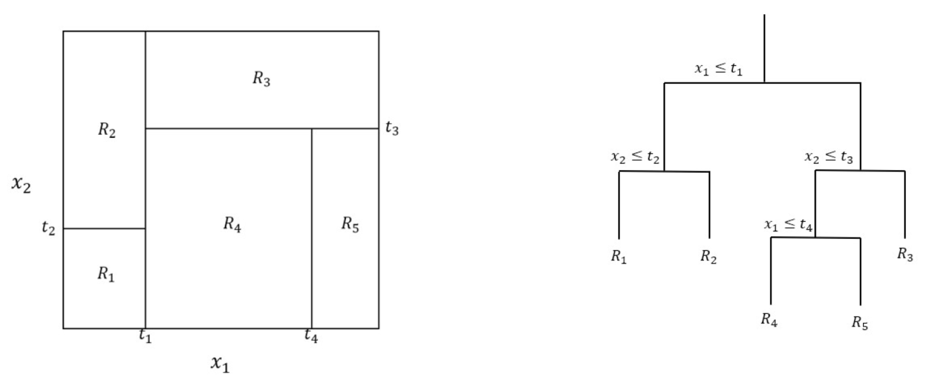
Tree-based methods work by partitioning the input space in a set of rectangles and then fitting a model in each partition using a decision rule. The partitions are built in a way that minimizes a specific metric (such as residual sum of squares for regression trees or the Gini index for classification trees), recursively, until a predetermined criterion is met (such as a minimum number of occurrences left in each partition). Predictions are performed depending on the partition the predictor variable falls in: often the mean or mode of the response training data in that partition for regression trees or the most frequent class for classification ones [32,33]. Because the process can often lead to overfitted trees, an additional step called “tree pruning” is performed, aiming to remove partitions, usually with a penalty based on the number of nodes in a specific level of the tree, although different algorithms can be used. Figure 1 presents the partitions for a hypothetical bivariate dataset and its respective tree structure.
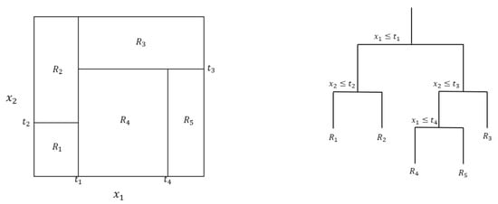
Figure 1.
Representation of a hypothetical decision tree for a bivariate problem. Left: results from a recursive binary split of a bivariate space; Right: the respective tree representation of the left structure.
Tree based models are very interpretable and relatively easy to explain, as they can be represented graphically [33]. They also can better handle categorical variables and strategies can be implemented to deal with missing values. Trees, however, usually do not have the same prediction accuracy as other models and tend to be very non-robust, having high variance. In order to improve the performance of decision trees, an ensemble-based method called random forests was developed.
“Random forests” is the name given to an ensemble meta model proposed by Breiman [34] composed of multiple decision trees. It uses the principle of bagging (bootstrap aggregation), which is a general-purpose procedure for reducing the variance of a learning method [33]. On random forests, E trees are trained on E bootstrapped samples and either the average of the prediction results of each individual tree (for regression settings) or the most commonly occurring class (for classification settings) is taken as the prediction. The main difference between bagging and random forests is the predictor subset size: In bagging, all the features are used, while on random forests, a smaller subset is adopted, leading to a lower correlation between trees, improving the accuracy [33]. While each individual tree has high variance, averaging the E trees leads to a reduction in that variance in exchange for a slight increase in the bias, thus improving the overall model accuracy.
2.2.4. Gradient Boosting
Boosting is the name given to a general method whose aim is to improve the accuracy of a learning algorithm [35]. It works by providing “weak” or “base” learner models a different subset of the training dataset, building an ensemble of weak learners, and combining their predictions in some way, instead of using a single result [35,36]. The original procedure proposed by Schapire [37] for binary classification used three learners, where the first learner was trained on a subset of the dataset (without replacement) to obtain the first classifier; the second learner was trained on a second subset of the dataset, including half of the misclassified samples from the first classifier, to produce the second classifier; the third learner was trained on all samples from the dataset in which the first and second classifiers disagreed, to produce the third classifier; and finally, the final classifier is one that uses the majority vote (mode) of the three trained classifiers. Additionally, the error can be further reduced by making the classifiers boosted learners themselves, in a recursive procedure. In the following years, many new algorithms and improvements were proposed for the methodology, including one proposed by Schapire himself called adaptive boosting, or AdaBoost, where weighted versions of the same training data are used instead of random samples [36].
One of the proposed algorithms that uses the boosting method is stochastic gradient boosting (also known as gradient boosting machine, or GBM), developed by Friedman [38]. Similar to random forests, it builds an ensemble of decision trees, with the difference that the models are trained in an additive iterative fashion. Starting from a single weak learner and given M total iterations, at each iteration m, a new learner will be trained so that
In other words, at each new iteration, a new attempts to improve the prediction of the previous model. Because to improve one needs to measure how well the model fits the data, for a given loss function that provides such measuring, the purpose of the algorithm is to minimize such a function. Hence, for each observation in the training dataset, the gradient of the loss function is calculated with respect to the associated prediction. That is,
Equation (7) presents the derivative of the loss function when the logistic loss is used (often the case for binary classification problems, although other loss functions can be used). For each observation, a new pair will exist (the gradient is also called “pseudo-residual”). The new learner is trained on those pairs, which will provide a decision tree structure. Next, one needs to determine the correction that will be applied on the values that fall inside each different region (also called partition or leaf) of the decision tree (refer to Figure 1), or , where ‘j’ represents each region of the trained decision tree . For classification problems, it can be calculated as shown in Equation (8):
In practice, Equation (6) is approximated using some kind of numerical method (such as Newton–Raphson). What it is calculating is basically a ‘correction’, an offset value that minimizes the loss in each region , and that will be the value returned by for each , as the objective is to find precisely that correction given each tree trained in each iteration m. This means that Equation (6) can be rewritten as (Equation (9)):
Hence, each different region of the tree will have its corresponding correction value that will be applied on each point that falls inside it. In practical contexts, a learning rate can also be added to control the size of the step in the gradient descent. The final model will be the sum of the learners. The GBM model and its variants can perform well on structured data, sometimes outperforming random forests, although it may need careful tuning of its hyperparameters, which may be a computationally intensive task.
2.2.5. Support Vector Machines
Support vector machines (SVMs) are maximum-margin mathematical models that extend the concept observed in the support vector classifier, by enlarging the feature space through the use of kernels [33]. While the support vector classifiers estimate a linear hyperplane to separate, in binary classification cases, two classes by minimizing the classification error within the boundaries, it suffers when the relationship between the predictors and response is non-linear. By using kernels, a function that quantifies the similarity of two observations, it is possible to estimate non-linear decision frontiers that better fit complex relationships present in the data. The SVM model has the following form (Equation (10)):
where ‘S’ is the collection of indices from the dataset, and the estimated parameters, and the kernel function, which can assume different formats. For example, in the case of a polynomial kernel, it has the following format (Equation (11)):
where ‘d’ is the degree of the polynomial function. If , the SVM has a linear kernel, and becomes the support vector classifier. For values of , the decision frontier becomes non-linear and more flexible. SVM has the advantage of being less computationally intense than simply transforming the feature space, allowing infinitely dimensional functions, such as the radial basis function kernel, to be used [32].
2.3. Imbalanced Data and Its Implications
A dataset is considered imbalanced when the sample size in the data classes is unevenly distributed [39] or, in other words, when it contains more occurrences from one class than the others [13]. For binary classification problems, Vluymans [15] argues that the uneven distribution of observations can be measured by the imbalanced ratio (IR), which is the ratio between the size of the majority class (often considered the negative class, ‘N’ or ‘0’) and the size of the minority class (considered the positive class, ‘P’ or ‘1’). The higher the value of IR, the more imbalance exists between the two classes. Values of IR greater than 1.5 indicate that the dataset is imbalanced, while values equal or greater than 9 indicate high imbalance.
Imbalanced datasets are common in real world problems and can adversely affect the performance of classification models. While most models work well with balanced training data if enough data are provided, issues arise when the datasets are imbalanced, as the standard learning methods used to train the models assume a balanced class distribution and, when those are not, the models tend to be biased towards the majority class [14,25,39]. The reason for that rests in the lack of representativity of the minority class: Due to the domination of the majority one, traditional training algorithms will generate imbalanced results, classifying most occurrences in the majority class, which will result in models with high accuracy for that class and close to zero for the minority one [40]. It is worth mentioning that the effect of several common data-related problems, such as sample representativity, high dimensionality, noise, and lack of density, can be potentialized in imbalanced datasets [15]. As the degree of concept complexity of the phenomenon being modeled increases, so does the system’s sensitivity to imbalance [41].
López et al. [25] evaluates that the solutions for the imbalanced dataset problem can be categorized in three groups: data sampling, where the data used to train the model is subjected to a pre-processing technique whose objective is to improve the balance between classes; algorithmic modification, where the training procedures of the classification models is altered in order to consider the imbalance between classes; and cost-sensitive learning, where a penalty to the misclassification of the minority class is applied, penalizing prediction errors in that class more than the errors in the majority one. A very popular algorithm belonging to the data sampling group is the SMOTE (synthetic minority over-sampling technique), proposed by Chawla et al. [42], and its variants.
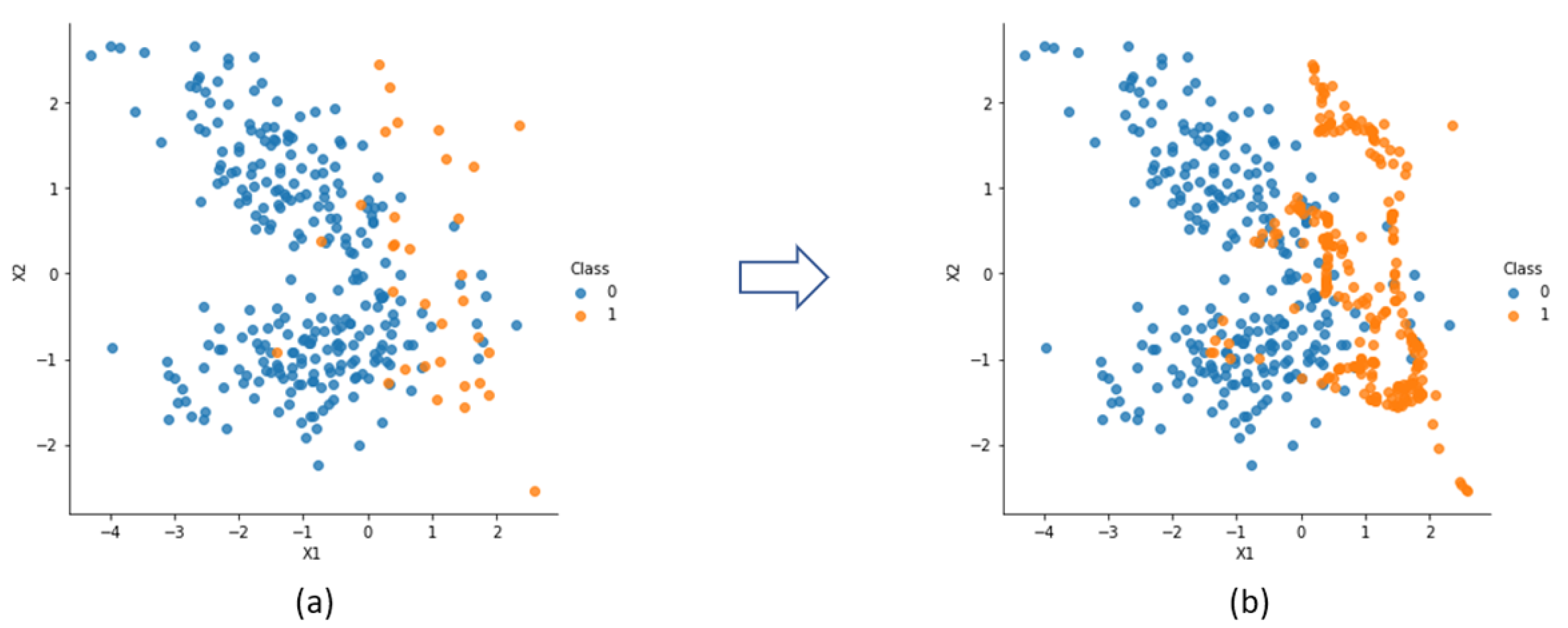
SMOTE is an oversampling approach in which the minority class is populated using artificially created occurrences, instead of being oversampled with a replacement, as carried out in random oversampling [42]. The algorithm can be described by a number of steps [42,43]. First, the total amount of oversampling N is defined, which depends on the IR desired (the aim may be a 1:1 ratio or another proportion). Then, an occurrence from the minority class is selected randomly. After, its k nearest neighbors (k can be defined beforehand, 5 by default) are identified and, finally, N of the k instances are chosen, randomly, to insert the new examples. Those are computed by interpolation, by calculating the difference between the occurrence and its neighbor, multiplying it by a random number between 0 and 1 and adding it to the occurrence vector. Figure 2 exemplifies the method, applied on a randomly generated bivariate binary dataset with 300 occurrences and a ratio of 10:1, until a ratio of 1:1 was reached, making the frontier between classes more evident.
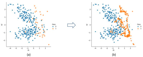
Figure 2.
SMOTE algorithm applied on an artificially generated dataset: (a) original dataset; (b) dataset after insertion of synthetic examples.
SMOTE was proposed as a solution to the overfitting problem present in the random oversampling method and, additionally, it allows for the decision boundaries of the minority class to spread further inside the majority class [44]. However, due to the way synthetic examples are created without consideration for the neighboring occurrences, the application of SMOTE can result in an overgeneralization of the minority class, leading to an overlap between different classes [15,25].
3. Materials and Methods
The observations in the dataset originated from an underground zinc mine that used vertical retreat mining, a variant of the sublevel open stoping, as the mine method. Each observation corresponds to a stope mined in the period between 2017 and 2020. From the descriptive features present in the dataset, those selected were the ones whose impact in stope stability has been consolidated in the literature:
- Rock Quality Designation (RQD) (%): RQD is defined as the ratio between the sum of the lengths of core fragments greater than 10 cm and the total length of the core run, preferably not exceeding 1.5 m [22,45]. Based on the obtained value, the rock mass will be classified in terms of its quality, ranging from very poor (0–25%) to excellent (90–100%). Various studies in the literature, using RQD or other classification systems, point to the influence of the rock mass quality on the stability of the opening, with higher-quality rock masses exhibiting greater stability [2,7,46,47].
- Hydraulic Radius (HR) (m): The hydraulic radius is defined as the ratio between the stope’s area of the hangingwall surface and its perimeter, a variable representing the geometry of the stope, a shape factor of the critical face [47]. The hydraulic radius was widely used in some of the earliest studies [1,2,6] related to stope stability, with a trend of decreasing stability as its value increases [48].
- Depth (m): According to Hoek et al. [49], the vertical stress applied to a rock mass can be estimated from the product of the depth of a point within that rock mass by its specific weight. In the mine under consideration, the specific weight of the rock mass is considered approximately constant (about 28 kN/m3), meaning that vertical stress is directly proportional to depth. Different studies [8,50] suggest that the relaxation and redistribution of stresses applied to the rock mass are influential variables affecting the stability of the stope.
- Direction (degrees): This refers to the direction of the hangingwall’s surface plane, i.e., its orientation relative to north. The orientation of the stope with respect to the discontinuity sets present in the rock mass is a critical factor for its stability [5,6].
- Dip (degrees): Dip is the angle between a plane parallel to the hangingwall and a horizontal plane of reference. Stopes with less steep dips tend to exhibit greater instability, as vertical stresses are directed onto the orebody, resulting in larger displacements within the rock mass [10].
- Undercut (m): This variable refers to the situation where the shape of the drift leading to the stope does not follow the ore contact and extends into the hangingwall [51]. Undercutting is an influential factor in stope stability because it degrades the integrity of the rock mass and increases the zones of loosened rock that could potentially fall into the stope [7]. Here, the value represents the performed undercut by the mine operations team.
- Stability factors: Three correction factors are multiplied by the Q-value from Barton’s Q-system [3] to calculate the stability number ‘N’ used in the Matthews [1] and Potvin [2] stability charts. Factor A represents the effect of stress on the stope surface, Factor B is associated with the effect of discontinuities on the stability of that surface, and Factor C evaluates the effect of gravity on the stope surface.
The response variable is binary, representing the classification of the stope as either unstable or stable. The criterion for defining stope stability followed that used by Clark [6] and by Qi et al. [12] in their studies. Based on the evaluation of ELOS (equivalent linear overbreak slough), measured using a cavity monitoring system (CMS), it was proposed that stopes with an ELOS value greater than 1 m would be considered unstable, while those with an ELOS value less than 1 m would be considered stable.
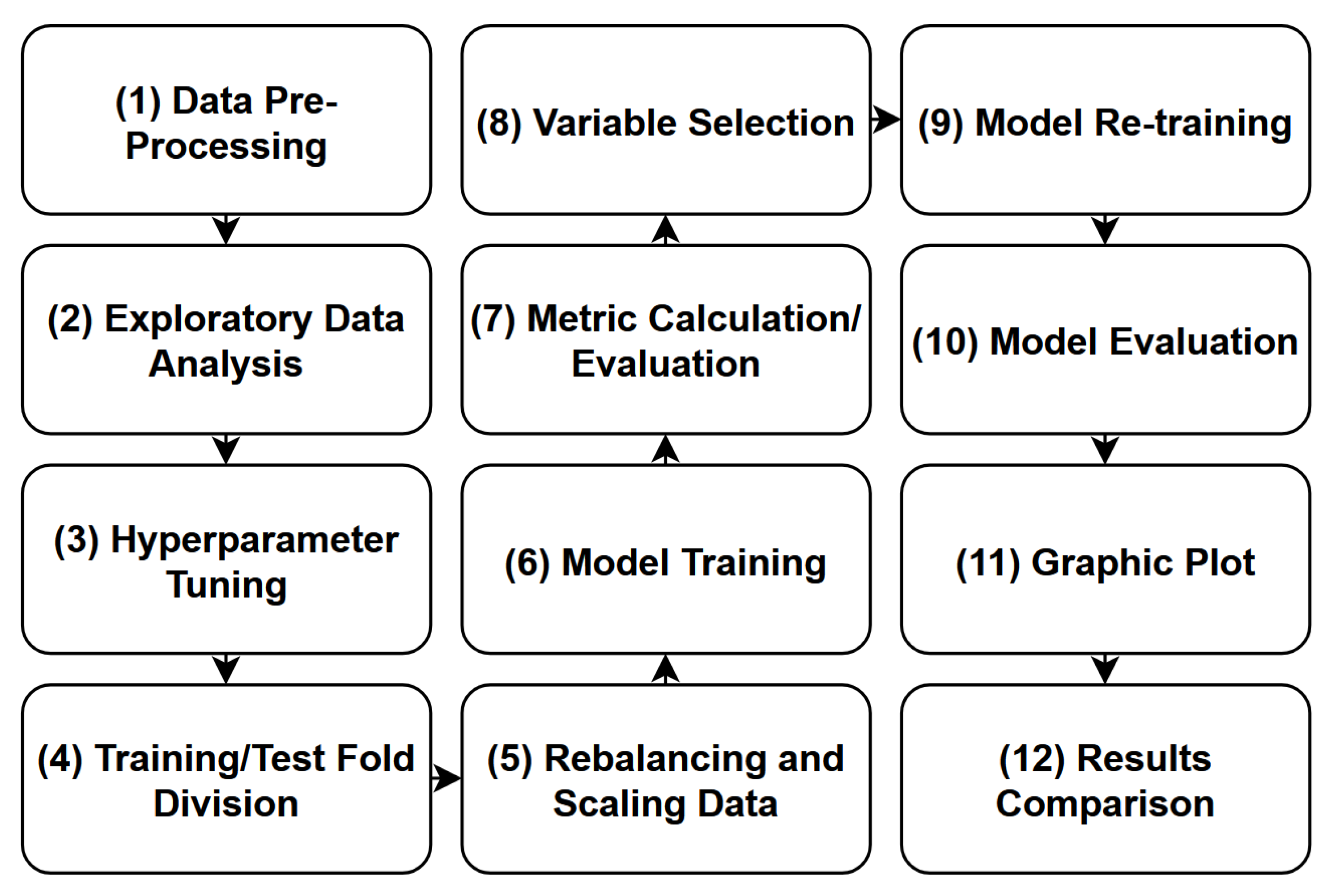
As an analytical tool, the Python 3.7 programming language and its available libraries were used. The adopted process flow is summarized in Figure 3.
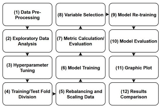
Figure 3.
Flowchart of the steps adopted in the modeling process.
The data pre-processing stage involved selecting the variables considered relevant to the process, determining the variable types, and investigating the presence of null and duplicate values. The exploratory analysis included univariate analysis, which involved evaluating descriptive statistics by considering the observations in each class separately, as well as assessing features distributions. It also included bivariate analysis, which involved investigating correlations between the variables.
The model hyperparameter selection and tuning was performed using the “grid search” method, which conducts an exhaustive search within defined subsets of the possible hyperparameter space [52]. In total, five models were trained and tested. Data rebalancing was performed using the SMOTE algorithm, whereas the scaling was performed using the z-score. To evaluate model performance, four different metrics were used: accuracy, precision, recall, and G-mean, although the G-mean was the standard metric adopted in loss functions and hyperparameter tuning. Variable selection was performed using the permutation feature importance method [53] on the G-mean metric.
For dividing the dataset into training and testing sets, the “k-fold cross-validation” methodology was used. In this approach, the dataset is subdivided into k subsets such that are used to train the models and 1 is used for testing. The subsets are rotated through these roles until all observations have been used in both the training and testing processes. A value of was adopted in this procedure. The subdivision into subsets is carried out randomly but maintains the class proportions in the different subsets (“stratified k-fold”). The cross-validation procedure is widely adopted as a method for estimating a model’s predictive error [32].
The five models evaluated were logistic regression, k-nearest neighbors, random forests, gradient boosting machine, and support vector machine. Models were chosen based on their characteristics: Logistic regression is a simple but highly interpretable model that, when used as a classifier, estimates a linear frontier that separates the classes; k-nearest neighbors is the most simple non-parametric classification algorithm, being highly flexible in the frontier estimation; random forests and gradient boosting machines are, respectively, bagging and boosting-type models, which allows them to work well in regard the bias-variance tradeoff; and the support vector machines are also highly interpretable and flexible models that can estimate different frontiers depending on the kernel used.
- Logistic regression: The hyperparameters tuned using grid search were the regularization parameter “C” (in increments of a factor of 10, ranging from 0.001 to 1000) and the norm used in the penalty (“l1” or “l2”). The optimal combination found to maximize the G-mean was and norm = “l1”.
- k-nearest neighbors: The only adjusted hyperparameter was the number of nearest neighbors “k” (ranging from 1 to 200). The value found that maximized the G-mean was .
- Random forest: The tuned hyperparameters were the maximum depth of the decision trees (an integer ranging from 3 to 10), the number of decision trees in the model (an integer increasing in steps of 50 from 50 to 1000), and the selection criterion (Gini or entropy). The combination that maximized the G-mean was a depth of 5, number of trees = 200, and criterion = “entropy”.
- Gradient boosting machine: The weak learners were decision trees and the tuned hyperparameters were the number of estimators (an integer, ranging from 50 to 500, in steps of 50), the learning rate (a float ranging from 0.1 to 1 in steps of 0.1) and the maximum depth (integer, from 0 to 10). The combination that maximized the G-mean was number of estimators = 150, learning rate = 0.8, and maximum depth = 3.
- Support vector machine: The tuned hyperparameters were the model’s kernel (“Gaussian RBF”, “sigmoidal”, and “polynomial”), the regularization parameter “C” (multiples of 10, ranging from 0.001 to 1000), and the Gamma parameter (multiples of 10, between 0.001 and 1). The combination that maximized the G-mean was kernel = “polynomial” (with degree = 3), , and gamma = 0.01.
It is worth mentioning that the list is not exhaustive and was constrained by the computational power available to run the grid search algorithm in feasible time. Some of the optimal values were also observed to present slightly different results after the algorithm was executed multiple times due to the probabilistic nature of the process and effects of imbalance in the testing dataset. The ranges for hyperparameters were chosen as recommended by the Scikit-learn Python library user guide [54].
4. Results and Discussion
A preliminary investigation of the database indicated the presence of 341 observations and 22 variables, out of which 10 were selected for the study following the previously presented guidelines. None of these variables showed any null occurrences. A single duplicate observation was identified and promptly removed. All 10 variables were renamed to facilitate interpretation, processing, and recognition by the programming language, as shown in Table 1.

Table 1.
Variables as identified in the programming code.
For statistical analysis purposes, all presented variables will be considered continuous numerical variables acting as predictors, with the exception of the ‘state’ variable, which serves as the response variable. The latter will be considered a non-ordinal categorical discrete variable with a cardinality of 2, taking the value ‘0’ when the stope is considered stable and ‘1’ when the stope is considered unstable—note that the study’s purpose is to be able to predict stope instability (hence, the positive class). Once the initial assessment of the database was completed, the exploratory data analysis of the predictors began. Table 2 and Table 3 present the descriptive statistics of the predictor variables for stable and unstable stopes, respectively.
Table 2.
Descriptive statistics for the stable stopes.
Table 3.
Descriptive statistics for the unstable stopes.
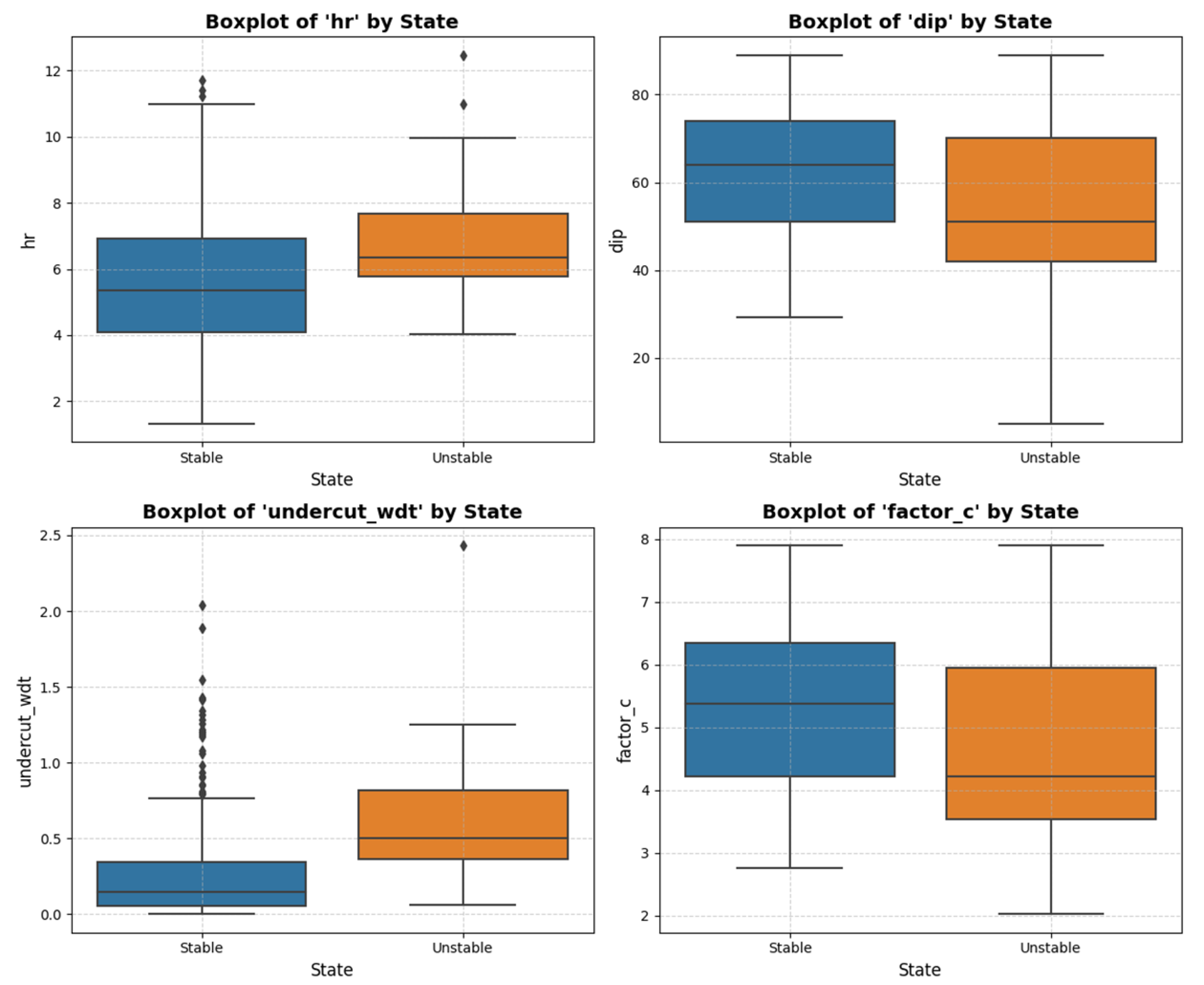
From the count of observations in the different classes, it can be noted that the database is highly imbalanced, with an IR (imbalance ratio) equal to 15.2. That is contrasts with other works in the literature such as Potvin’s [2], with an IR of approximately 2.4; Clark’s [6], with an IR of approximately 2.6; and Wang’s [7], with an IR higher than 1.5. For RQD, unstable stopes have a lower average value than stable ones, which aligns with the literature (although, perhaps, within the expected variability). A similar conclusion can be drawn for the hydraulic radius, where the average for unstable stopes tends to be higher. Comparable values for the mean and quartiles of stope depth in both classes indicate that they have similar distributions across sublevels, potentially suggesting that this variable, on its own, may not have strong discriminative power. Dip and undercut are also in line with findings from the literature, with steeper stopes tending to be more stable and stopes with greater undercut tending toward instability. Factors A and B appear to have similar distributions between the classes, suggesting limited potential in the classification process, while for Factor C, stopes with lower values seem to tend toward instability.
Another important aspect to investigate is the similarity between the distributions in different classes. Since the purpose of a classifier is to estimate a decision boundary that separates observations belonging to different categories, variables whose class distributions are clearly distinct tend to contribute more, individually, to the classification process. One way to investigate this difference is through the Mann–Whitney U test [55], a non-parametric hypothesis test that allows one to determine whether the distribution that generated a particular sample “x” is the same as that which generated a particular sample “y”. Thus, by applying the test on the variables in different classes, the p-value for the test statistic can be seen in Table 4.
Table 4.
p-Value for the test statistic from Mann–Whitney test.
It can be concluded that it is possible to reject the null hypothesis for some of the variables—“hr”, “dip”, “undercut_wdt”, and “factor_c”—indicating that these variables, individually, contribute more significantly to differentiating between the classes. However, the univariate analysis does not allow us to determine whether there are any complex relationships among the remaining variables. Therefore, all nine were retained for the modeling process. The discriminative characteristics of the four aforementioned variables can be more readily visualized with a boxplot, as shown in Figure 4.
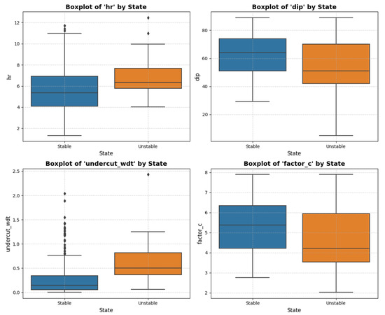
Figure 4.
Boxplots of the variables ‘hr’, ‘dip’, ‘undercut_wdt’, and ‘factor_c’.
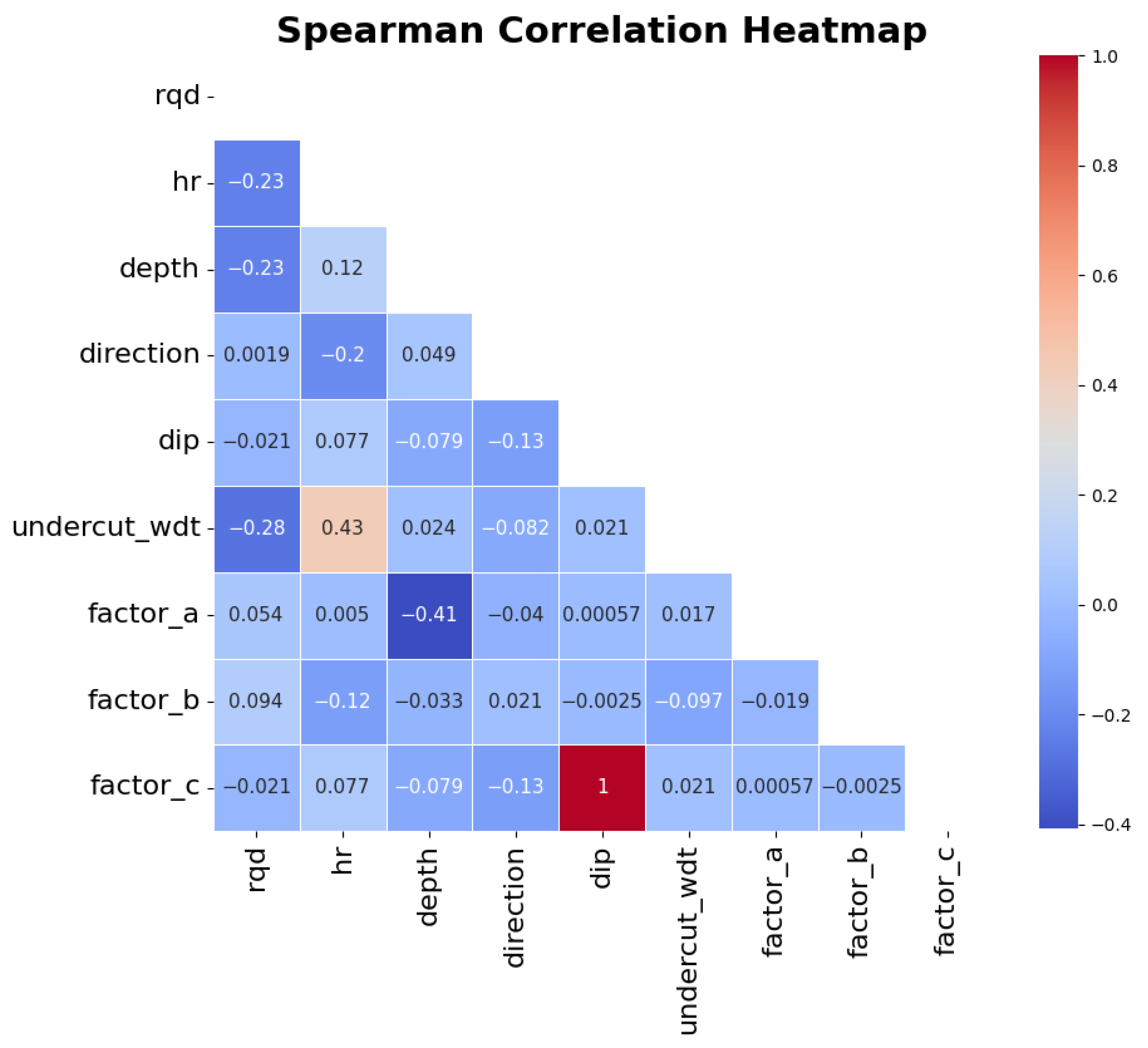
By examining the relative positioning of the boxplots representing the observations in different classes, a distinction between the distributions can be observed, which is particularly notable for the variable ‘undercut_wdt’. To evaluate the correlation between the variables, correlation coefficients can be employed. For this work, the Spearman correlation coefficient was chosen because it can also detect monotonic nonlinear relationships between the variables. The results can be seen in Figure 5.

Figure 5.
Correlation heatmap for the Spearman correlation coefficient between predictor variables.
Most of the features present a weak to no correlation with each other. A noticeable exception is the variable ‘dip’, which shows a strong correlation with the variable ‘factor_c’, although something expected given ‘factor_c’ uses the value of stope dip on its calculation. Other relevant relationships observed are between ‘factor_a’ and ‘depth’, which present a moderate negative relationship, something also in line with the literature given that ‘factor_a’ is inversely proportional to the vertical stresses applied on the rock mass which, in turn, increase with the depth; and between the ‘undercut_wdt’ and ‘rqd’, which present a moderate positive relationship. This last one, however, is unexpected: It can potentially mean that there is a tendency in the mine of opening larger stopes in areas where the undercut is greater or, in the other way, that the undercut tends to be higher in areas where larger stopes are planned. The investigation and confirmation of those, however, is outside the scope of this work currently. Additionally, although retaining correlated variables can incur bias in certain models, their impact is negligible when using the models for prediction (which is the purpose of this work) rather than for inference; hence, it was opted to keep both the correlated variables in the subsequent steps.
With the exploratory analysis completed, the training and testing of the models began. Table 5 presents the average value of the metrics on the five train-test folds from the cross-validation after the models were trained on the original dataset, without rebalancing, whereas Table 6 presents the same, but after the training dataset was rebalanced with the SMOTE algorithm [42] (testing sets do not get rebalanced) until an I.R. of 1 was reached (as hyperparameter, the algorithm used k, the number of neighbors, equal to 3).
Table 5.
Average results of the five folds for the evaluation metrics (imbalanced training dataset).
Table 6.
Average results of the five folds for the evaluation metrics (rebalanced training dataset).
It is important to clarify the meaning of the metrics in the context of the stability phenomena in order to better evaluate the results. First, accuracy: Because it is a metric that evaluates the correctness of the algorithm, it is expected that it will be high when the dataset is imbalanced as the model will simply classify all stopes as stable and, because the number of stable observations is much higher than unstable, the mistakes made on the unstable have little effect on the metric value itself. That is the reason why the metric can be misleading, as a model that considers every stope as stable is useless in a stability evaluation context.
Now, for precision and recall: In a model trained on an imbalanced dataset, both will tend to have very low values or zero, which is expected as the value in the numerator in both metrics is the number of unstable stopes correctly classified as unstable. Because classifiers trained on imbalanced datasets are unable to correctly identify unstable stopes, that value will tend to be zero, bringing the whole metric to zero. When the dataset is rebalanced, the scenario changes: The precision will increase, albeit the results remain low. That is because precision has the false negative on the denominator (see Equation (1)) and, as the dataset is rebalanced, a portion of the estimated decision frontier will invade the region of the stable stopes, making the classifier consider those as unstable. As for recall, the value has a significant boost, which is expected as the number of unstable stopes correctly classified increase with the rebalancing, as the decision frontier becomes clearer for the classifier. The G-mean is the metric with highest increase: Influenced by the classifier’s capability of identifying both the stable and unstable stopes, the metric tends to increase as the model manages to better identify the unstable ones, even though it will be penalized by mistaking some stable stopes as unstable.
In a mining context, the decision regarding which model to use will depend on the business strategies: Mines at high risk of instability will most likely lean more towards models with high recall. Other metrics may also be used, such as the F-beta score (harmonic mean between precision and recall, where recall weights ‘beta’ times more) or balanced accuracy. Metrics can also be improved for a given classifier by changing the threshold of the decision rule. It is also possible to create custom metrics based on different mistaking costs, using a function on a cost-sensitive learning process. Those, however, are beyond the scope of this paper.
The next step involved selecting the two most relevant variables for the classification process. Was chosen for the task permutation feature importance, an algorithm that shuffles the observations on each feature individually and measures the average impact on a metric of choice used. The metric evaluated was the G-mean and the results are presented in Table 7. Green cells represent the feature with the highest G-mean decrease (and its value) for the given model, whereas the yellow cells represent the feature with the second highest G-mean decrease.
Table 7.
Average decrease in G-mean upon variable shuffling through permutation feature importance.
The first aspect of notice is the removal of the feature “dip” in the results: “dip” was identified as being highly correlated with “factor_c”, something expected as the latter uses the former to be calculated. While correlated variables have a negligible impact on the predictive capabilities of the models, the same can not be said for the usage of permutation importance, because although the features are shuffled individually, the model would still have access to the information through the corresponding correlated feature, leading to a bias that results in lower importance values for both features. Hence, it was decided to maintain “factor_c” instead of “dip”. As for the values themselves, the higher the value, the greater the impact shuffling the variable has on the model’s performance. Negative values imply that either the variable is detrimental to the model or some slight improvement was observed on chance alone.
Regarding the results, different models will be capable of processing the features differently. Green cells represent the highest value for a given model, whereas yellow cells represent the second highest. The predominance of “undercut_wdt” as the most impactful feature in four of the five models is noticeable. The relevance of “undercut_wdt” as a discriminant variable had been previously identified during the exploratory data analysis (see Figure 4), with permutation importance further confirming the finding. Similarly, the hydraulic radius (“hr”) was identified as the second most impactful feature in three of the five models, evidencing the effect that the stope’s geometry may have on instability. Considering those findings, those two features will be the ones used in implementing the stability graphs. It is important, though, to highlight that those results are specific to the mine context in which the research was developed: Because stability is a complex phenomenon, different variables may reveal themselves as being impactful on different mines, so a context-specific analysis must be performed instead of over-relying on findings from external environments.
The results obtained also provide useful insight that goes beyond the stability graphs: Because the undercut width was identified as being a very impactful feature, it is possible to conclude that, for that specific mine, the stope stability is strongly related to operational performance when building the drifts on which the stopes will be drilled, highlighting the importance of increased control in operational procedures. The hydraulic radius, as a representative of the stope geometry, also plays a role for mine planning in determining the maximum size of the stope. Other variables that were identified as relevant, albeit to a lesser degree, such as the dip, may also help in stope development on specific circumstances.
The models were, then, trained one last time with the two most impactful features identified, “hr” and “undercut_wdt”. Training was performed on 80% of the dataset (after rebalancing), whereas the testing (on which the metrics were calculated upon) was performed on the remaining 20% (original observations, unbalanced). The results are presented on Table 8.
Table 8.
Evaluation metrics for models trained on the two most impactful features.
Generally, an improvement was observed after the removal of certain variables, which may be expected given that some values observed in Table 7 are either zero or negative, with little to no contribution towards the classification process (or even harmful). Logistic regression presents the highest values across the metrics, which may infer the linear nature of the estimated Bayes decision frontier. A highlight is the performance of the support vector machine, in which there was a drop in the G-mean, which is also expected considering that the model identified other features as being more impactful.
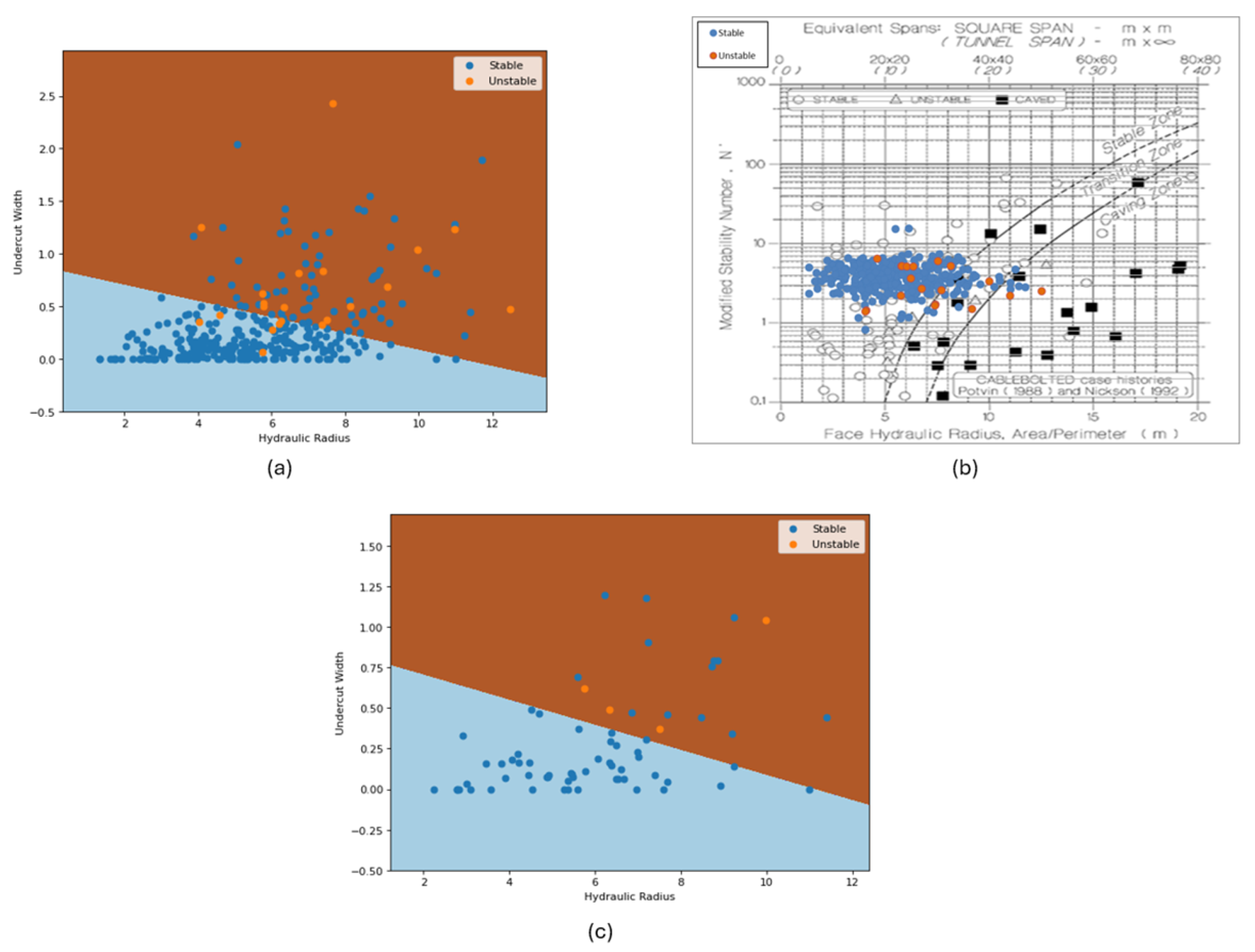
The hypothesis defined before this study is that, through probabilistic modeling, it is possible to implement a more accurate and site-specific stability graph to trump the traditionally used one developed by Matthews and Potvin. Following the principle of Occam’s razor, the logistic regression model was chosen as the deliverable of comparison. Figure 6 presents three graphs: (a) represents the estimated decision frontier (with the brown area representing the unstable zone and the blue area, the stable one) with all the dataset plotted (dark blue points represent the stable stopes and orange points represent the unstable ones); (b) represents the Mathew and Potvin’s graph when all the dataset is plotted on it (note that the modified stability number, N’, provided by the mine’s geotechnical team was used, instead of the undercut width values); and (c) represents the same decision frontier present in (a), but with only the test dataset plotted.

Figure 6.
Stability graphs: (a) logistic regression model graph with the full dataset plotted; (b) Mathews and Potvin graph (after Potvin, 1988 [2] and Nickson, 1992 [18]) with the full dataset plotted; (c) logistic regression with only the training dataset plotted.
The first element to be observed is the nature of the graphs. While in Figure 6a, there are only two zones, stable and unstable, Figure 6b also considers a transition zone. It is worth mentioning that the methodology proposed also allows the inclusion of a transition zone (or as many as the model engineer wishes), but those must be defined using objective criteria. Then, there is the accuracy: It is noticeable that Figure 6b classifies far more unstable stopes as stable (and a few as transition, which is hard to evaluate in this context), making over-reliance on it risky when used for mine planning in mines that suffer from stability issues or as an argument to reinforce the need for additional support in specific areas of the mine. The plot in Figure 6c has as the purpose of evaluating the real potential of the developed graph when used to evaluate future observed stopes, as it uses data “unseen” by the algorithm during the training process: For the specific iteration on which the frontier was estimated, the model performed reasonably well on unstable stopes (remembering that only 20% of the dataset was used), managing to correctly classify all the unstable observations, although some stable stopes were misclassified. It is important to highlight the random nature of the process: Due to the high imbalance present in the dataset, different iterations may bring drastically different results, and while such high variance does not invalidate the process, it does reinforce the need for more data. Finally, Figure 7 presents the decision frontiers estimated by the other models.
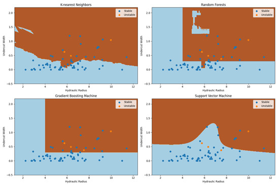
Figure 7.
Stability graphs generated by the other models, K-nearest neighbors, random forests, gradient boosting machine, and support vector machine, and plot of the training dataset.
The estimated decision frontiers reflect the nature of the different algorithms used to generate them. The value of the hyperparameter k used in K-nearest neighbors will control the flexibility of the frontier, with lower values generating more flexible (albeit possibly “noisy”) frontiers. The value used (48) can be considered reasonably high in comparison to the size of the training dataset, so that may be the reason the estimated frontier is somewhat “rough” and close to the linear one estimated by the logistic regression model. Random forests and gradient boosting are both models that have decision trees at their core, and classify the observations by partitioning the domain space, the reason why the decision frontiers look like “boxes”. In the RF model, a peculiarity can be observed: the presence of a strangely placed stable zone amidst the unstable one. As it is unlikely that the trend of instability was broken in that specific place, such a peculiarity is most likely due to random variance present in the training dataset (potentially, a few isolated stable stopes are located there). Due to the bagging nature of the random forest model, situations like those may be solved by modifying the model’s hyperparameters. Regarding the support vector machine, the estimated frontier will be dependent on the kernel used: The smooth “curvy” aspect is due to the usage of a third-degree polynomial kernel.
As a final comment, the choice of the “best” stability graph may depend on more than model performance: Interpretability is an important factor, with graphs that provide clearer and understandable zones being preferable if performances are similar. Data availability is also important: Graphs that are built on specific features that may be expensive or hard to measure accurately may penalize the decision-making process in the long-term usage of the graph, with a similar notion valid for the use of features whose impact in the stability phenomenon may be hard to grasp, or that are hard to act upon or control, given that one of the main purposes of the graph is to provide professionals a tool to evaluate the impact of relevant aspects pertinent to stability so that mine planning may be adjusted accordingly and adequate corrective/containment measures may be taken.
5. Conclusions and Future Work
Conclusively, it was possible to validate the original hypothesis that it is possible to build a reasonably accurate, site-specific stability graph through statistical and machine learning modeling. The models, in general, outperformed Mathews and Potvin’s graph, particularly in identifying unstable stopes, even when trained on a highly imbalanced dataset, which makes them even more promising to develop in more adequate, balanced ones.
However, it is important to highlight that it is not a silver bullet: It depends on a dataset that represents adequately the phenomenological domain of stability for the specific mine site on which it is based upon, as evidenced by how the impact of imbalance affected the performance of all models (although some models may be more robust to it), and rebalancing algorithms should be used as a last resort, given they may not be able to correctly adjust the dataset to be adequately representative of the domain for the algorithms if the stability phenomenon in the mine is overly complex. The data quality is also a big concern: Some of the variables that may be used in investigating stability (including some not used here, such as Barton’s Q system) may be prone to subjectivity in their measurement, especially when performed by different professionals, something that can significantly impact the results. This is also valid for the response variable or label: In this study, the label was defined by discretizing the ELOS measurement using an objective criterion. Defining which stopes are stable or unstable using subjective analysis (such as “individual experience”) may end up not generating an adequate dataset that can be used for modeling. Finally, it is highly desired that all the stopes involved belong to the same population, meaning that all the observations belong roughly to the same probabilistic distribution: As an example, if the characteristics of the rock mass change drastically as the mine develops, it may be more adequate to perform a new exploratory data analysis, separate the stopes, and update the graph-generating model accordingly, as using data from different populations may have a detrimental impact on the model’s capacity to estimate the decision frontier (again, some are more robust to those deviations).
As for future work, several different improvements are suggested. Some models (such as random forests and GBM) are highly dependent on hyperparameter tuning. The method chosen, grid search, being a hard heuristic, ensures that the best combination within the specified subset is found. However, that does not mean that the identified subset is globally best, and increasing the size can be very computationally intensive, so other optimization methods, such as Bayesian optimization, may be tested to better tune the models. There is also the loss of information due to the removal of features: In this study, the variables were limited to two for the sake of interpretability, but depending on the mine site, the instability phenomenon may be highly influenced by more than two features. In this case, using an approach such as PCA (principal component analysis) may be worth evaluating, although a graph built on the vectors estimated by the algorithm may not have the same level of interpretability as using the standalone features. Another aspect is the estimated decision frontier: By standard, the criteria chosen in this study were to estimate the one closest to the Bayes decision frontier. However, depending on the business strategy of some mines, different weights may be given for classification mistakes, so a study that proposes some strategy to define the most adequate decision frontier based on specific business rules could be an interesting prospect. There is also the stability phenomenon itself: During this study, the observations were considered independent (which is an assumption for the models used); however, the stopes can be considered as being spatially correlated (as subsequent openings can also affect previous ones) and time correlated (as the stability status of a given stope may change with time, given the redistribution of the forces), so understanding how those characteristics can be modeled may help improve the graph development process, being particularly relevant for mines that have dynamic data flows, allowing for real-time updating of the stope stability status. Also, investigating how the graph behaves in different mining contexts is a desirable future prospect.
Author Contributions
Conceptualization, L.d.A.G.P. and E.B.d.J.; Methodology, L.d.A.G.P.; Software, L.d.A.G.P.; Validation, W.P.R.; Formal analysis, L.d.A.G.P.; Investigation, L.d.A.G.P.; Resources, L.d.A.G.P. and E.B.d.J.; Data curation, L.d.A.G.P.; Writing—original draft, L.d.A.G.P.; Writing—review & editing, W.P.R. and E.B.d.J.; Visualization, W.P.R. and E.B.d.J.; Supervision, W.P.R. and E.B.d.J.; Project administration, E.B.d.J. All authors have read and agreed to the published version of the manuscript.
Funding
This research received no external funding.
Data Availability Statement
The data used in this study can be made available on request, depending on permission from the company that owns it.
Conflicts of Interest
The authors declare no conflicts of interest.
References
- Mathews, K.E.; Hoek, E.; Wyllie, D.C.; Stewart, S.B.V. Prediction of Stable Excavation Spans for Mining at Depths Below 1,000 Meters in Hard Rock; Technical Report; Report to Canada Centre for Mining and Energy Technology (CAANMET), Department of Energy and Resources, Ottawa, ON, Canada; Golder Associates: Toronto, ON, Canada, 1980. [Google Scholar]
- Potvin, Y. Empirical Open Stope Design in Canada. Ph.D. Thesis, University of British Columbia, Vancouver, BC, Canada, 1988. [Google Scholar]
- Barton, N.; Lien, R.; Lunde, J.J.R.M. Engineering classification of rock masses for the design of tunnel support. Rock Mech. 1974, 6, 189–236. [Google Scholar] [CrossRef]
- Laubscher, D.H. A geomechanics classification system for the rating of rock mass in mine design. J. S. Afr. Inst. Min. Metall. 1990, 90, 257–273. [Google Scholar]
- Villaescusa, E. Excavation design for bench stoping at Mount Isa mine, Queensland, Australia. Trans. Inst. Min. Metall. Sect. A Min. Ind. 1996, 105, A1–A10. [Google Scholar]
- Clark, L.M. Minimizing Dilution in Open Stope Mining with a Focus on Stope Design and Narrow Vein Longhole Blasting. Ph.D. Thesis, University of British Columbia, Vancouver, BC, Canada, 1998. [Google Scholar]
- Wang, J. Influence of Stress, Undercutting, Blasting and Time on Open Stope Stability and Dilution. Ph.D. Thesis, University of Saskatchewan, Saskatoon, SK, Canada, 2004. [Google Scholar]
- Stewart, P.C. Minimising Dilution in Narrow Vein Mines. Ph.D. Thesis, University of Queensland, Brisbane, Australia, 2005. [Google Scholar]
- Germain, P.; Hadjigeorgiou, J. Influence of stope geometry and blasting patterns on recorded overbreak. Int. J. Rock Mech. Min. Sci. 1997, 34, 115.e1–115.e12. [Google Scholar]
- Henning, J.G.; Mitri, H.S. Numerical modelling of ore dilution in blasthole stoping. Int. J. Rock Mech. Min. Sci. 2007, 44, 692–703. [Google Scholar]
- Suorineni, F.; Papaioanou, A.; Baird, L.; Hines, D. A dilution-based stability graph for open stope design. In Proceedings of the 7th International Conference and Exhibition on Mass Mining, Sydney, Australia, 9–11 May 2016; The Australasian Institute of Mining and Metallurgy: Sydney, Australia, 2016; pp. 511–522. [Google Scholar]
- Qi, C.; Fourie, A.; Du, X.; Tang, X. Prediction of open stope hangingwall stability using random forests. Nat. Hazards 2018, 92, 1179–1197. [Google Scholar]
- Estabrooks, A.; Jo, T.; Japkowicz, N. A multiple resampling method for learning from imbalanced data sets. Comput. Intell. 2004, 20, 18–36. [Google Scholar] [CrossRef]
- Japkowicz, N. The class imbalance problem: Significance and strategies. In Proceedings of the International Conference on Artificial Intelligence (IC-AI 2000), Las Vegas, NV, USA, 26–29 June 2000; Volume 56, pp. 111–117. [Google Scholar]
- Vluymans, S. Dealing with Imbalanced and Weakly Labelled Data in Machine Learning Using Fuzzy and Rough Set Methods; Springer: Berlin/Heidelberg, Germany, 2019; Volume 107, p. 236. [Google Scholar]
- Dzimunya, N. Geotechnical Study on the Feasibility of Using Backfill in Steep Dip Areas of Konkola Copper Mines (Zambia). Ph.D. Thesis, The University of Zambia, Lusaka, Zambia, 2017. [Google Scholar]
- Mawdesley, C.; Trueman, R.; Whiten, W. Extending the Mathews stability graph for open–stope design. Min. Technol. 2001, 110, 27–39. [Google Scholar]
- Nickson, S.D. Cable Support Guidelines for Underground Hard Rock Mine Operations. Ph.D. Thesis, University of British Columbia, Vancouver, BC, Canada, 1992. [Google Scholar]
- Hadjigeorgiou, J.; Leclair, J.; Potvin, Y. An update of the stability graph method for open stope design. In Proceedings of the CIM Rock Mechanics and Strata Control Session, Halifax, NS, Canada, 14–18 May 1995; Volume 14, p. 18. [Google Scholar]
- Stewart, P.C.; Trueman, R. Strategies for Minimising and Predicting Dilution in Narrow-Vein Mines—NVD Method; Australasian Institute of Mining and Metallurgy: Carlton, Australia, 2008. [Google Scholar]
- Suorineni, F.T. The stability graph after three decades in use: Experiences and the way forward. Int. J. Min. Reclam. Environ. 2010, 24, 307–339. [Google Scholar]
- Deere, D. The rock quality designation (RQD) index in practice. In Rock Classification Systems for Engineering Purposes; ASTM International: West Conshohocken, PA, USA, 1988. [Google Scholar]
- Pérez-Ortiz, M.; Jiménez-Fernández, S.; Gutiérrez, P.A.; Alexandre, E.; Hervás-Martínez, C.; Salcedo-Sanz, S. A review of classification problems and algorithms in renewable energy applications. Energies 2016, 9, 607. [Google Scholar] [CrossRef]
- He, H.; Garcia, E.A. Learning from imbalanced data. IEEE Trans. Knowl. Data Eng. 2009, 21, 1263–1284. [Google Scholar]
- López, V.; Fernández, A.; García, S.; Palade, V.; Herrera, F. An insight into classification with imbalanced data: Empirical results and current trends on using data intrinsic characteristics. Inf. Sci. 2013, 250, 113–141. [Google Scholar] [CrossRef]
- Daskalaki, S.; Kopanas, I.; Avouris, N. Evaluation of classifiers for an uneven class distribution problem. Appl. Artif. Intell. 2006, 20, 381–417. [Google Scholar] [CrossRef]
- Branco, P.; Torgo, L.; Ribeiro, R.P. A survey of predictive modeling on imbalanced domains. ACM Comput. Surv. CSUR 2016, 49, 1–50. [Google Scholar] [CrossRef]
- Kubat, M.; Holte, R.C.; Matwin, S. Machine learning for the detection of oil spills in satellite radar images. Mach. Learn. 1998, 30, 195–215. [Google Scholar] [CrossRef]
- Kotsiantis, S.; Kanellopoulos, D.; Pintelas, P. Handling imbalanced datasets: A review. GESTS Int. Trans. Comput. Sci. Eng. 2006, 30, 25–36. [Google Scholar]
- Kim, M.J.; Kang, D.K.; Kim, H.B. Geometric mean based boosting algorithm with over-sampling to resolve data imbalance problem for bankruptcy prediction. Expert Syst. Appl. 2015, 42, 1074–1082. [Google Scholar] [CrossRef]
- Kleinbaum, D.G.; Dietz, K.; Gail, M.; Klein, M.; Klein, M. Logistic Regression; Springer: New York, NY, USA, 2002; p. 536. [Google Scholar]
- Hastie, T.; Tibshirani, R.; Friedman, J. The Elements of Statistical Learning: Data Mining, Inference, and Prediction; Springer: New York, NY, USA, 2017. [Google Scholar]
- James, G.; Witten, D.; Hastie, T.; Tibshirani, R.; Taylor, J. An Introduction to Statistical Learning: With Applications in Python; Springer Nature: New York, NY, USA, 2023. [Google Scholar]
- Breiman, L. Random forests. Mach. Learn. 2001, 45, 5–32. [Google Scholar] [CrossRef]
- Schapire, R.E. A brief introduction to boosting. In Proceedings of the International Joint Conference on Artificial Intelligence (IJCAI), Stockholm, Sweden, 31 July–6 August 1999; Volume 99, pp. 1401–1406. [Google Scholar]
- Ferreira, A.; Figueiredo, M. Boosting algorithms: A review of methods, theory, and applications. In Ensemble Machine Learning: Methods and Applications; Springer: New York, NY, USA, 2012; pp. 35–85. [Google Scholar]
- Schapire, R.E. The strength of weak learnability. Mach. Learn. 1990, 5, 197–227. [Google Scholar] [CrossRef]
- Friedman, J.H. Stochastic gradient boosting. Comput. Stat. Data Anal. 2002, 38, 367–378. [Google Scholar] [CrossRef]
- Boughorbel, S.; Jarray, F.; El-Anbari, M. Optimal classifier for imbalanced data using Matthews Correlation Coefficient metric. PLoS ONE 2017, 12, e0177678. [Google Scholar] [CrossRef] [PubMed]
- Tang, B.; He, H. GIR-based ensemble sampling approaches for imbalanced learning. Pattern Recognit. 2017, 71, 306–319. [Google Scholar] [CrossRef]
- Sun, Y.; Wong, A.K.; Kamel, M.S. Classification of imbalanced data: A review. Int. J. Pattern Recognit. Artif. Intell. 2009, 23, 687–719. [Google Scholar] [CrossRef]
- Chawla, N.V.; Bowyer, K.W.; Hall, L.O.; Kegelmeyer, W.P. SMOTE: Synthetic minority over-sampling technique. J. Artif. Intell. Res. 2002, 16, 321–357. [Google Scholar] [CrossRef]
- Fernández, A.; Garcia, S.; Herrera, F.; Chawla, N.V. SMOTE for learning from imbalanced data: Progress and challenges, marking the 15-year anniversary. J. Artif. Intell. Res. 2018, 61, 863–905. [Google Scholar] [CrossRef]
- Batista, G.E.; Prati, R.C.; Monard, M.C. A study of the behavior of several methods for balancing machine learning training data. ACM SIGKDD Explor. Newsl. 2004, 6, 20–29. [Google Scholar] [CrossRef]
- Deere, D.; Hendron, A.; Patton, F.; Cording, E. Design of surface and near-surface construction in rock. In Proceedings of the ARMA US Rock Mechanics/Geomechanics Symposium, Minneapolis, MN, USA, 15–17 September 1966. [Google Scholar]
- Villaescusa, E. Geotechnical design for dilution control in underground mining. In Proceedings of the Mine Planning and Equipment Selection, Calgary, AB, Canada, 6–9 October 1998; pp. 141–149. [Google Scholar]
- Abdellah, W.; Hefni, M.; Ahmed, H. Factors influencing stope hanging wall stability and ore dilution in narrow-vein deposits: Part 1. Geotech. Geol. Eng. 2020, 38, 1451–1470. [Google Scholar] [CrossRef]
- Heidarzadeh, S. Probabilistic Stability Analysis of Open Stopes in Sublevel Stoping Method by Numerical Modeling. Ph.D. Thesis, Université du Québec à Chicoutimi, Chicoutimi, QC, Canada, 2018. [Google Scholar]
- Hoek, E.; Kaiser, P.K.; Bawden, W.F. Support of Underground Excavations in Hard Rock; CRC Press: Boca Raton, FL, USA, 2000. [Google Scholar]
- Capes, G.W. Open Stope Hangingwall Design Based on General And Detailed Data Collection in Unfavourable Hangingwall Conditions. Ph.D. Thesis, University of Saskatchewan, Saskatoon, SK, Canada, 2009. [Google Scholar]
- Costa, L.; de Figueiredo, R. Methodology to Predict and Reduce the Unplanned Dilution in Narrow Vein Underground Mines. Case study: Córrego do Sítio Mine–Santa Bárbara–MG, Brazil. In Proceedings of the ISRM Congress, Foz do Iguaçu, Brazil, 13–18 September 2019. [Google Scholar]
- Syarif, I.; Prugel-Bennett, A.; Wills, G. SVM parameter optimization using grid search and genetic algorithm to improve classification performance. TELKOMNIKA Telecommun. Comput. Electron. Control 2016, 14, 1502–1509. [Google Scholar] [CrossRef]
- Altmann, A.; Toloşi, L.; Sander, O.; Lengauer, T. Permutation importance: A corrected feature importance measure. Bioinformatics 2010, 26, 1340–1347. [Google Scholar] [CrossRef]
- Scikit-Learn User Guide. Available online: https://scikit-learn.org/stable/user_guide.html (accessed on 11 November 2024).
- Mann, H.B.; Whitney, D.R. On a test of whether one of two random variables is stochastically larger than the other. Ann. Math. Stat. 1947, 18, 50–60. [Google Scholar] [CrossRef]

Disclaimer/Publisher’s Note: The statements, opinions and data contained in all publications are solely those of the individual author(s) and contributor(s) and not of MDPI and/or the editor(s). MDPI and/or the editor(s) disclaim responsibility for any injury to people or property resulting from any ideas, methods, instructions or products referred to in the content. |
© 2025 by the authors. Licensee MDPI, Basel, Switzerland. This article is an open access article distributed under the terms and conditions of the Creative Commons Attribution (CC BY) license (https://creativecommons.org/licenses/by/4.0/).