Review

VNIR-SWIR Imaging Spectroscopy for Mining: Insights for Hyperspectral Drone Applications

by
Friederike Koerting
1,*,
Saeid Asadzadeh
2,
Justus Constantin Hildebrand
1,
Ekaterina Savinova
3,
Evlampia Kouzeli
4,
Konstantinos Nikolakopoulos
4,
David Lindblom
5,
Nicole Koellner
2,
Simon J. Buckley
6,
Miranda Lehman
7,
Daniel Schläpfer
8 and
Steven Micklethwaite
3
1
Norsk Elektro Optikk AS—HySpex Division, Østensjøvei 34, 0667 Oslo, Norway
2
Helmholtz Centre Potsdam, GFZ German Research Centre for Geosciences, 14473 Potsdam, Germany
3
Sustainable Minerals Institute, The University of Queensland, St. Lucia, QLD 4067, Australia
4
GIS and Remote Sensing Lab, Department of Geology, University of Patras, 26504 Patras, Greece
5
Prediktera AB, 907 36 Umeå, Sweden
6
Independent Researcher, 5008 Bergen, Norway
7
Center to Advance the Science of Exploration to Reclamation in Mining, Department of Geology and Geological Engineering, Colorado School of Mines, Golden, CO 80401, USA
8
ReSe Applications LLC., 9500 Wil, Switzerland
*
Author to whom correspondence should be addressed.
Mining 2024, 4(4), 1013-1057; https://doi.org/10.3390/mining4040057
Submission received: 16 July 2024 / Revised: 7 November 2024 / Accepted: 21 November 2024 / Published: 29 November 2024

Abstract

:
Hyperspectral imaging technology holds great potential for various stages of the mining life cycle, both in active and abandoned mines, from exploration to reclamation. The technology, however, has yet to achieve large-scale industrial implementation and acceptance. While hyperspectral satellite imagery yields high spectral resolution, a high signal-to-noise ratio (SNR), and global availability with breakthrough systems like EnMAP, EMIT, GaoFen-5, PRISMA, and Tanager-1, limited spatial and temporal resolution poses challenges for the mining sectors, which require decimetre-to-centimetre-scale spatial resolution for applications such as reconciliation and environmental monitoring and daily temporal revisit times, such as for ore/waste estimates and geotechnical assessments. Hyperspectral imaging from drones (Uncrewed Aerial Systems; UASs) offers high-spatial-resolution data relevant to the pit/mine scale, with the capability for frequent, user-defined re-visit times for areas of limited extent. Areas of interest can be defined by the user and targeted explicitly. Collecting data in the visible to near and shortwave infrared (VNIR-SWIR) wavelength regions offers the detection of different minerals and surface alteration patterns, potentially revealing crucial information for exploration, extraction, re-mining, waste remediation, and rehabilitation. This is related to but not exclusive to detecting deleterious minerals for different processes (e.g., clays, iron oxides, talc), secondary iron oxides indicating the leakage of acid mine drainage for rehabilitation efforts, swelling clays potentially affecting rock integrity and stability, and alteration minerals used to vector toward economic mineralisation (e.g., dickite, jarosite, alunite). In this paper, we review applicable instrumentation, software components, and relevant studies deploying hyperspectral imaging datasets in or appropriate to the mining sector, with a particular focus on hyperspectral VNIR-SWIR UASs. Complementarily, we draw on previous insights from airborne, satellite, and ground-based imaging systems. We also discuss common practises for UAS survey planning and ground sampling considerations to aid in data interpretation.

1. Introduction

Remote sensing (RS), especially imaging spectroscopy, offers large-scale, non-destructive, and time-efficient means for mapping mining environments, including mineral, lithology, soil, and plant species over spatially extensive areas at the deposit, camp, and outcrop scales. Imaging spectroscopy is based on the selective absorption and reflectance of wavelengths of light by different materials. In RS, both “hyperspectral imaging” (HSI) and “multispectral imaging” (MSI) are common methods used in Earth observation applications. In geological studies, electromagnetic radiation (EMR) is often focused on the visible to near-infrared (400–1000 nm; VNIR) and the short-wave infrared (1000–2500 nm; SWIR) [1] is utilised to detect mineral-specific absorption features. Reviews on the fundamentals have been covered by, e.g., Clark [1], Van der Meer et al. [2], Hunt [3,4,5], Hecker et al. [6], and Manolakis et al. [7].
The term “mining” is used widely in public discourse. In this paper, we use the term “mining” to refer specifically to the process of exploring for and producing metals or rock aggregate materials, from open-pit operations and the resulting by-products and post-mining landscapes. Satellite-borne RS data, together with field-based (close-range) sensing systems (handheld hyperspectral point spectrometers) have played a key role during green- and brownfield exploration programmes for mining. From an exploration perspective, spectral imaging is a relatively mature technology used to map spectrally active minerals, e.g., in the alteration footprints of hydrothermal mineral systems. However, once a project enters the operational phase, spectral RS technology is not widely employed for mineral identification and mapping. In this phase, the common RS nadir perspective (bird’s eye view) of airborne and satellite sensors needs to be complemented by drone-borne and ground-based scanning systems to cover steep vertical walls that are poorly imaged by orbital sensors.

1.1. Uncrewed Aerial Systems in Mining

The term Uncrewed Aerial Vehicle (UAV) mainly describes the aircraft itself, whereas Uncrewed Aerial System (UAS) is used throughout this document to refer to the complete aircraft system, including the control module, navigation hardware, transmission systems, cameras, software, ground station, and person(s) controlling the vehicle, which is colloquially often referred to as a “drone”.
The versatility of deploying a UAS has led to its increased adoption within the mining sector. This largely involves applications based on RGB imagery and photogrammetry in stockpile volume surveying, site infrastructure inspections, and some environmental monitoring. However, the UAS has the potential to act as interoperable technology with a broad range of applications that include geological pit mapping [8], geotechnical analysis, geophysical survey, rock slope stability assessment, water quality monitoring, erosion and soil loss estimation, Acid Mine Drainage (AMD) mapping, subsidence detection and safety management (e.g., tailings dams, road haulage, etc.), and post-mining environmental monitoring [9,10]. In complex environments within the mining value chain, the need for Digital Terrain Models (DTMs) of high accuracy and high spatial resolution can be fully addressed with a UAS equipped with light detection and ranging (LiDAR) technology [11]. This capability can be applied in landslide mapping [11,12,13,14,15,16,17,18,19], slope monitoring [20,21,22,23], subsidence modelling [24]), and surface models [17,25,26,27]). While an important tool, LiDAR alone lacks information on surface composition and is only considered an additional instrument to HSI in this manuscript.
With advanced sensor technology, relatively lightweight hyperspectral sensors have recently emerged covering the entire VNIR and SWIR regions of the electromagnetic spectrum. Capturing data across these wavelength regions via UASs enables the mapping of a variety of materials over mining sites at high spatial resolution [28,29]. To date, hyperspectral cameras for UASs spanning the mid-wave infrared (MWIR; 3000–5000 nm) or long-wave infrared (LWIR; 7000–14,000 nm) are not available. While numerous papers have covered the use of UAS technology in the mining industry, only a few have included case studies of hyperspectral UASs [30,31,32,33,34,35,36,37,38,39,40,41,42,43,44,45]. Although several reviews have focused on the application of hyperspectral imaging and RS in the broader field of geology [2,4,5,30,31,32,33,34], there is a notable absence of a comprehensive review on the state-of-the-art methods for HSI and its applications within mining, both in active and post-mining environments. We focus on the application of emerging UAS-based HSI technology, but we also review case studies conducted using airborne and spaceborne imaging systems to understand the full potential of UASs in the mining industry and recognise the niche that UASs could fill.
New hyperspectral spaceborne missions provide higher spectral resolution than ever before. One impediment of satellite missions is limitation in the spatial resolution of the data that do not exceed 30 m so far [35]. A UAS, equipped with a spectral imaging instrument, can bridge this gap and provide high-spectral and high-spatial resolution data simultaneously. For instance, tailings and AMD-prone surfaces have been analysed mostly via airborne and UAS-borne HSI data of high spatial resolution, due to the manageable spatial extent of these surfaces, the spatial resolution of associated surface patterns, and the need for monitoring at a higher temporal frequency than what satellites allow, such as after relevant precipitation events. If larger areas require coverage, airborne HSI is the method of choice, due to the currently limited airtime of UAS HSI.
We believe that some additional factors contribute to the currently limited utilisation of UAS HSI data within the mining industry:
  • The sparse availability of commercial turn-key solutions, outside of core scanning systems covering both the data acquisition and analysis/interpretation.
  • Difficulties in sensing the vertical faces of a mine (which is currently being addressed by ground-based and UAS-based systems). Though ground-based solutions (tripod-based) have provided data on vertical faces, their deployment in an open-pit environment is at best prototypical. Some truck-mounted systems have been deployed, suggesting safer practises at open-pit sites.
  • The inability of 3D modelling software systems (e.g., Datamine, MinePlan, Leapfrog, Vulcan) (at least until recently) to take spatial, (semi-)quantitative mineralogical data into account, deal with complex colour-coding and display legends for 4D spectral data.
  • Concerns about the repeatability of data over the highly dynamic mining sites and seasonally variable surfaces (e.g., AMD). The consistency of the data over time is a challenge that has yet to be addressed fully.
  • Methodological limitations for time-relevant data acquisition, visualisations, and processing. Current techniques of data acquisition and processing are still labour-intensive, costly, and time-consuming and heavily rely on the expertise of the interpreter.
  • A lack of service providers in the mining space to offer, e.g., UAS-based HSI data collection and interpretation to non-expert users.
  • A shortage of well-documented and publicly available case studies with quantified, validated results and clear value propositions.

1.2. State-of-the-Art Methods and Progress of UAS-Based HSI in Mining

We believe that identifying the state of the art in deploying spectral imaging within mining environments is the first step for these projects to identify the remaining challenges and opportunities and find solutions to fully integrate hyperspectral imaging in the mining industry as a standard tool. Governmental and industry projects are currently addressing the challenges and developing solutions toward higher technology readiness levels (TRLs). For example, EU- and national-funded projects are underway, deploying UASs in the context of the critical mineral strategy and the European Raw Materials Initiative. One of these projects is the M4Mining project (Multi-scale, Multi-sensor Mapping and dynamic Monitoring for sustainable extraction and safe closure in Mining environments, www.m4mining.eu, accessed on 1 February 2024) funded by the European Union. This project aims to develop solutions for HSI UASs, identify data analyses, and set standards for the mining industry, to enable an end-user-ready hardware and software solution. While individual hardware building blocks and subsystems to be integrated in the UAS monitoring system are all available as commercial products at TRL 9 (systems proven in an operational environment), the integration itself, for oblique data acquisition and real-time analysis, has yet to be developed. Research projects like M4Mining aim to develop a solution that reaches TRL 5 (technology validated in a relevant environment) or higher to ensure quick integration into the mining industry by service providers or miners themselves. Providing these systems to miners enables them, among other things, to make decisions at a higher certainty and provide another level of security to stakeholders, collect spatial data on mineralogy over sites of interest, aid mine planning, and comply with environmental monitoring guidelines.
In this paper, we summarise spectral imaging principles (Section 2) and review existing case studies of HSI applied in the mining sector, including airborne and spaceborne platforms, to highlight the potential applications for hyperspectral UAS (Section 3). We present common hyperspectral UAV systems and discuss the design of hyperspectral UAS campaigns (Section 4), including sampling and validation standards. We then conclude with a discussion of possible future applications of the technology in the mining value chain (Section 5). By discussing both the advantages and the current state of hyperspectral VNIR-SWIR UAS, as well as describing best practises for HSI UAS campaign planning, we hope to provide a practical account of the potential and challenges of using HSI UAS in mining and provide support for geoscientists interested in applying HSI UAS to their projects.

2. Principles of Spectral Imaging

Imaging spectroscopy is usually referred to when measurements and analysis are taken out with hyperspectral instruments. In RS, both “hyperspectral imaging” (HSI) or “multispectral imaging” (MSI) are common methods used in Earth observation applications. Here, discussing both methods, we will use the term “spectral imaging”. In geological studies, electromagnetic radiation (EMR), either in the VNIR, SWIR, MWIR, or thermal infrared (5500–15,000 nm; TIR), is sensed by passive camera systems. The wavelength ranges in the SWIR, MWIR, and TIR follow the definitions in [36]. Geological RS studies often denote the LWIR as part of the TIR. While LWIR offers the advantage of detecting rock-forming minerals such as quartz and feldspar [36], the focus of the review is on the VNIR-SWIR region with UAS-mountable cameras in that region.
Geological remote sensing took off with the deployment of the Airborne Visible/infrared Imaging Spectrometer (AVIRIS) and other airborne and spaceborne instruments such as HyMap, Hyperion, Landsat series, ALI, ASTER, and WorldView-2 and -3 [30,37,38,39,40,41,42,43,44]. Data from these platforms, especially freely available data, became popular with exploration geologists for both green- and brownfield projects, such as over remote, vast landscapes at medium (5 m) to low (30 m) spatial resolutions. These instruments collected either MSI (for the above-mentioned instruments, up to 10 different wavelength bands offering low spectral resolution) or HSI data (collecting information in hundreds of narrow consecutive bands to resolve narrow spectral features). Satellite remote sensing, using ultra-high resolution true-colour RGB imagery with a spatial resolution in the cm—dm range, offers some utility for the mining industry, especially when mapping smaller-scale changes. This includes monitoring surface changes on the surface of tailings, detecting surface expressions of subsidence, and mapping mining footprints and activities [45,46,47,48]. Nonetheless, since these systems are limited to visible wavelengths, they cannot be used to distinguish surface mineralogy apart from visible colour.
HSI, due to high spectral resolution, can resolve narrow absorption features specific to different minerals and materials. While the definition of “hyperspectral” in terms of number of bands is not rigid, the Institute of Electrical and Electronics Engineers (IEEE) Standards Association set up a standard in 2018 for devices that cover the 0.25–2.50 µm spectral region. For a system to be considered hyperspectral, it needs to exceed 32 bands as per the IEEE P4001—Standard for Characterization and Calibration of Ultraviolet through Shortwave Infrared (250 Nm to 2500 Nm) Hyperspectral Imaging Devices. [49]. In this context, any instrument that captures less than 32 spectral bands is considered multispectral.
Imaging spectroscopy generates data cubes where each image pixel represents four-dimensional information, with three dimensions in the spatial x-, y, and z-coordinates, and spectral information in the fourth dimension. Data cubes are created using the principles of spectroscopy, where the properties of light are captured across a set of continuous spectral bands to produce a characteristic spectrum on a per-pixel basis. Pushbroom RS employs an array of detectors to capture spectral imaging data of the Earth’s surface as the platform moves [50,51]. Unlike whiskbroom systems that scan across a scene with a single detector, pushbroom systems capture entire lines of data simultaneously, offering high spatial and spectral resolution. This method minimises motion blur and enables efficient data collection by continuously recording data along the platform’s path, capturing multiple spectral bands simultaneously.

2.1. Spectral Data Analysis

With the use of VNIR and SWIR wavelength ranges, rock material from all stages of the mining value chain can be investigated by studying the characteristic absorption features, inflexions, and signature slopes of the individual (pixel) spectrum captured by the imaging system. In geological environments, absorption features detected in the VNIR arise from transitional elements, including iron-bearing minerals and rare-earth elements (REEs), while the SWIR region is commonly used for identifying alteration mineral assemblages related to hydrothermal systems of base and precious metal deposits [52]. The mineral groups that can be detected and mapped in the VNIR-SWIR wavelength regions include carbonates, sulphates, sulphosalts, clays, phosphates, and phyllosilicates such as chlorite, talc, and muscovite. A detailed account of the causes of absorption features can be found in [3,4,5].
Various analytical techniques are used to characterise, classify, and semi-quantify spectral features of minerals, rocks, or elements. Not one method provides an absolute answer; rather, each method highlights different patterns or nuances in the spectral data that are used as proxy for interpretation and classification. For this review, we withhold any discussions related to advantages and disadvantages of these methods for different applications and data sources. An overview of the spectral processing methods available for geological RS is provided in [2,4,5,30,31,32,33,34]. Several advantages and disadvantages as well as challenges in geological spectral characterisation and mapping methods are discussed therein, touching on topics such as overlapping spectral features, lack of clear correlation between absorption feature depth and mineral abundance, or the challenges of different geochemical and mineralogical validation methods for validated spectral mineralogy. It is also worth mentioning that HSI data in geology present challenges due to the high correlation and redundancy of spectral bands, which can complicate statistical modelling and increase computational demands. Methods such as dimensionality reduction are used to identify and retain the bands most sensitive to key spectral regions.
Common analytical techniques for imaging spectroscopic data are divided into two broad categories: (1) data-driven and (2) knowledge-based approaches [34]. Data-driven approaches rely only on the data and some additional reference data (spectra), commonly called training classes or endmember sets, that are imported to or derived from the image data. Data-driven approaches are categorised into per-pixel (hard classifier) and sub-pixel (soft classifier) approaches with single and multiple labels for each pixel, respectively. Comparison-based per-pixel approaches, such as spectral matching with the use of a reference spectral library, include similarity-based methods such as the Spectral Angle Mapper (SAM) [53,54,55], least squares-based methods such as least squares regression (PLSR), and learning-based approaches such as artificial neural networks (ANNs) [56,57], random forest (RF) [58], or support vector machines (SVMs) [59,60]. Mixture-based, sub-pixel categories include partial and full unmixing methods such as mixture-tuned matched filtering (MTMF) and linear spectral unmixing (LSU). The non-linear mixing of the data is addressed in many publications, typically concluding that the physical properties of the material are the reason for spectral mixing, while hardware plays a similarly significant role [61,62,63,64,65,66,67]. While spatial mixtures can be solved from an analytics perspective, hardware optimisation plays an equal role in solving this challenge. Spatial misregistration in the hardware is an enormous contributor to non-linear spectral signature mixing and requires consideration at all processing steps. Knowledge-based approaches rely on user knowledge about the spectral behaviour of a target without the use of direct reference data to extract meaningful information from a spectrum. Knowledge-based approaches aim to estimate the quality and/or quantity of either of the main components making up a spectrum including the following: (i) a continuum, (ii) absorption bands, and (iii) residuals or noise. These techniques include absorption and spectral feature modelling. A common feature mapping approach in this category is “minimum wavelength mapping” (MWL). This feature-based approach retrieves the depth, minimum wavelength, area, width, and asymmetry of individual features, known as spectral parameters, for material identification and mapping [6,36,68,69,70]. The output of this technique can be fed into expert systems and decision tree structures (DT) to enable per-pixel classification. Examples of expert systems include the classic USGS Tetracorder and its modern interface called the “Material Identification and Classification Algorithm” (MICA) [71,72,73]. Partial absorption modelling and clustering techniques [74], as well as various band arithmetics (e.g., band ratios), also do not require the use of pre-existing reference data. Applying these techniques results in spectral similarity and score images with varying magnitudes of the matched and inferred values and requires specialised visualisation and contextualisation methods to interpret the resulting output maps.

2.2. Auxiliary Data Acquisition

The collection of field data involves many stages and needs to be managed carefully for hyperspectral field campaigns, including UAS surveys. Field data typically include various instrument data, ancillary data (“metadata”), and geographic coordinates and images, which can lead to interrelated but disjointed datasets.
The terminology here follows that of the Terrestrial Ecosystem Research Network (TERN) “Effective Field Calibration and Validation Practices” [75]. Data are considered direct quantitative measurements of the sample in question, either via an instrument or another quantitative method (e.g., instrument readings, raw imagery). Ancillary data are considered data collected in association with the primary dataset such as geographical coordinates, comments, date and time, descriptive information, and imagery and information about the instruments being used. Metadata are considered the information regarding the discovery and the use of the data, such as scale, units, geographical and temporal scales, custodians, and licencing. The careful collection of this information is important to ensure that various researchers and stakeholders can reuse the data in the future.
Field calibration and sampling strategies for remotely sensed data have recently been developed for ecological applications and provide some utility for geoscientific surveys [75]. Clearly defined strategies are important as field surveys can be logistically challenging, especially for UAS-based HSI, influencing the quality of the survey data and associated ground sampling and calibration data. Based on the strategies developed for ecological applications, we suggest the following high-level considerations for geoscientific remote sensing studies: Firstly, field data collection can vary depending on the site access conditions and weather conditions. As a result of these factors, sampling strategies are often modified. Secondly, the equipment in larger campaigns can vary, as can the observers and their experience level, resulting in inconsistencies due to observer bias and different objectives. Consequently, we suggest the principle that all field methods must be discussed prior to any campaign and a consistent sampling strategy (e.g., number/density of samples, sample area dimensions, etc.) and the relevant protocols (e.g., calibration procedures, repeats, blanks, etc.) must be applied. We recommend the best practice suggested by TERN, such as the following: (1) the use of data entry tools to minimise errors, (2) providing sufficient data storage via an accessible and reliable database with clearly established data licences during and after a survey, and (3) establishing a frequent review period (annual) to identify issues, provide feedback on data completeness, and identify unbalanced data collection across sites and potential data bias.

3. Spectral Imaging Applied to the Resource Sector

The literature for this review was identified through a comprehensive approach, combining both systematic keyword-based searches and leveraging the scientific expertise and prior experience of the co-authors. Search terms such as “hyperspectral”, “VNIR”, and “SWIR”, were employed, in combination with “mining”, “geology”, “exploration”, “mine waste”, and “rehabilitation”, to ensure that relevant studies were identified across different thematic areas. These terms were selected based on their relevance to the study’s focus on UAS-based technologies from mineral exploration to mine waste management. This resulted in 112 studies to be included in the following review.
To date, UAS-based HSI data have been featured in only a few published case studies. However, there is a wealth of studies based on ground-based, airborne, and satellite-borne imaging spectroscopy in the mining sector, and their review can provide important lessons for the application and interpretation of UAS-based HSI data, given their close analogy. In the following section, relevant RS studies in the mining sector are reviewed and categorised based on different stages in the mining life cycle from exploration to the mining extraction, and finally closure and rehabilitation. Please note that while many of the referenced studies are based on platforms other than UASs, common outlook in the reviewed studies include the following:
(1)
Higher spatial resolution would benefit the method and interpretation and add value, and the outlook of published studies is often directly in favour of using UAS platforms, once available.
(2)
The use of a UAS can enable safer data acquisition compared to ground-based scanning and the acquisition of data in areas that cannot be reached by other methods
We therefore believe that the below-reviewed methods and their learnings directly benefit the future application of hyperspectral UASs in the mining sector.
A publication by Bedini, 2017 [30], reviewed the use of hyperspectral data for the mineral exploration of major deposit types. The author concluded that while magmatic and hydrothermal ore deposits have been studied extensively using hyperspectral technology, hydrothermal ore deposits in sedimentary environments, banded iron formations, sedimentary-rock hosted Mn deposits, and other ore deposits of sedimentary environments, as well as supergene ores, have no reported hyperspectral studies about them or only a limited number of studies. Porphyry copper and molybdenum, as well as epithermal gold deposits, are being characterised in detail using hyperspectral technology in many studies. This is likely because hydrothermal alteration minerals such as certain clays, phyllosilicates, and sulphates are spectrally active in the VNIR and SWIR and relevant to vector toward mineralized zones in these deposit types. Although previous work has focused on these deposit types, future applications are not limited to these. Learnings from earlier studies and previous laboratory and ground-based studies suggest that a variety of critical raw materials and aggregate mineral mining operations benefit from the use of hyperspectral UASs. Apart from the research mentioned in [30], Section 4 reviews additional hyperspectral imaging applied in exploration, operational mining and extraction, AMD detection, and environmental monitoring, rehabilitation, and revalorisation. In this review, we refer exclusively to open-pit mining and open-pit post-mining environments when discussing the use of hyperspectral UASs. Studies based on different platforms (ground-based, airborne, and satellite-borne) are then reviewed if they show potential to apply learnings for UAS HSI.
Here, we emphasise that the current review primarily focuses on the applications of spectral RS data in the mineral industry and does not cover the pictorial characteristics of high-resolution satellite data commonly utilised in the mining sector for logistics applications, land-change detection, and mapping (including topographic mapping). Appendix A lists the reviewed studies and puts them in the context of the area of application, used sensor and platform, and primary mapping objective (Table A1).

3.1. HSI Use in Mineral Exploration

Hyperspectral RS has traditionally been employed in mineral exploration, and the exploration sector is responsible for many published case studies over the past decades [37,41,76,77,78]. This has been accomplished mainly using airborne hyperspectral and/or satellite-borne multispectral datasets at various scales, with several studies focused on mineral mapping at a deposit scale. A well-documented example is the study of the Tertiary channel iron ore deposits in Rocklea Dome in the Hamersley region, Australia, covered by weathered/transported materials. Airborne, as well as surface and subsurface drill core, hyperspectral data (VNIR—SWIR) were used for 3D mineral mapping [79,80]. Through combining the surface and subsurface data, it was demonstrated that about 30% of exploration drill holes were sunk into the barren ground and could have been potentially avoided if airborne HSI had been consulted for drill hole planning to identify surface patterns pointing to mineralized channel deposits. A more recent study [81] used high-resolution airborne data (HyMap, 5 m spatial resolution) to map alteration mineralogy over a porphyry copper deposit in Iran to generate a drilling favourability map. HSI effectively mapped typical alteration minerals such as white mica, smectite, kaolinite, and ferric/ferrous minerals, which are all relevant for identifying proximity to metal mineralization. Table A1 in Appendix A provides a list of these currently available studies, including the application area and target minerals or relevant endmembers, as well as the imaging system used, method used, and data products. The new generation of spaceborne hyperspectral imaging methods such as PRISMA, EnMAP, EMIT, and GaoFen-5 (GF-5) are also well equipped for and predominantly used for mineral exploration and alteration/lithologic mapping purposes [76,82,83,84,85]. Yet, the high spectral resolution (<10 nm) and high SNR (>400:1) of these imaging systems can find numerous applications within the mining sector. A notable advantage of spaceborne imaging spectroscopy is its extensive coverage on a global scale. For instance, a single EnMAP scene encompasses approximately 1000 km2.
In contrast to ground-based hyperspectral imaging, which is still paving its way in the exploration sector, HSI is firmly established in core scanning technology in greenfield and brownfield exploration and has provided valuable lessons for high-resolution mineral mapping. Examples of where hyperspectral core scanning has been deployed include in Cu porphyry deposits [86,87], porphyry deposits alteration minerals [88,89,90], coal quality studies [91], Au-Cu-Zn volcanogenic massive sulphide (VMS) mineralisation [87,92,93,94], unconformity-related Uranium deposits [95], the analysis of basement rocks [96], the characterisation of REE-bearing minerals [97], material hardness for process optimisation in gold mining [98], and lithology discrimination in iron ore deposits [99]. In addition to these applications, hyperspectral core scanning offers significant potential for calibrating hyperspectral remote sensing in larger scales. Through linking high-resolution spectral data from core scanning, which can be validated via different geochemical or mineralogical methods, it is possible to create labelled, site-specific spectral libraries for classification purposes. For instance, spectral signatures from identified mineral phases, textural variations, and alteration patterns observed in core scans can be used as a baseline to refine remote sensing models and for understanding the effect of scale differences between <1 mm × 1 mm core scanning pixel sizes and a 10 cm × 10 cm mine face, and up to 30 m × 30 m satellite pixel sizes.

3.2. HSI Use in Operational Mining and Extraction Phases

HSI data have been used in various research studies during the extractive and active phases of mining. A ground-based HSI survey demonstrated how to find potential failure zones related to non-structural geological factors data by mapping the occurrence and extent of clay horizons, which are prone to failure and need to be monitored for stability [100]. Imaging spectroscopy has been used to detect harmful fugitive gas emissions (including but not limited to CO2 and CH4) from industrial processes to detect leaks [101,102], a capability that can be naturally extended to mining facilities and for remediation plans.
Few studies using HSI have been conducted at active mining environments and integrated spectral data into the mining process on a production basis. Most of these studies have relied on hyperspectral outcrop scanning as an established method to map surface mineralogy and lithology in natural rock outcrops and open-pit faces. While not embraced by the mining industry at large, it enables data-guided, close-to-face identification, and sorting by mapping quality (ore, waste, contamination) before or after blasting, and before the loading and transporting of the rock mass. Currently, due to the absence of an easily deployable HSI-UAS, a tripod-mounted hyperspectral camera enables the acquisition of an image from vertical faces This is often referred to as “ground-based” HSI. An overview of currently published case studies on ground-based mine face scanning gives insight for future UAS-based HSI studies [33]. The capability of VNIR-SWIR data for lithological mapping in outcrops has been explored for REE mineral, crude oil, and shale mapping in outcrops and samples via airborne HSI [103,104,105,106]. REE detection in outcrops in the FEN complex in Norway was performed by identifying narrow REE absorption features using noise reduction methods [107] in mining operations in the area. Long-range outcrop scanning (<1 km distance) was performed in the eastern Alaska Range to map outcropping porphyry deposits [108,109]. The automatic mapping of mine face geology has been published in combination with the LiDAR-based 3D modelling of open-pit surfaces [55,60,100,110]. Lithology and iron ore mapping in an unspecified open-pit mine in the Pilbara region in the VNIR spectral range was tested [60,111], as well as the mapping of mine faces in iron ore and gold mining using ground-based HSI [112]. Outcrops in a lithium–pegmatite mine in Northern Portugal were scanned using ground-based and UAS-based SWIR [113], and underground HSI outcrop mapping has been performed in several instances, e.g., to map clay materials to assess sealing properties in the Swiss Mont Terri rock laboratory [114] and in a Li-underground mine in Zinnwald/Cìnovec [115]. The first UAS-based, fully corrected, oblique, hyperspectral SWIR survey of an outcrop was published for limestone lithology [116]. A review of close-range, ground-based hyperspectral studies from 2019 [33] covers many of these studies in detail. White mica characterisation by HSI means was reviewed in [117] in relation to different deposit types such as base metal sulphide, epithermal, porphyry, orogenic gold, sedimentary rock-hosted gold, iron oxide copper gold, and unconformity-related uranium deposits. White mica chemistry and the white mica 2200 nm combination feature wavelength position are meaningfully connected. The wavelength position of white mica in Cresson Pit at the Cripple Creek & Victor mine in cripple creek, Colorado, USA, is mapped in Figure 1. The general trend toward longer wavelength positions due to lower Al content with increasing depth in the pit corresponds to increased proximity to the high-temperature causative intrusion at depth.
The first UAS-borne and tripod-based HSI study was performed in the context of geometallurgy in a small active copper mine and leach operation. It concluded that HSI can become a useful tool for detecting the distribution of clays and carbonates [118]. Clays are well distinguishable using HSI and are of interest in active mining environments as they affect recovery in flotation circuits and are responsible for lower permeability in leaching, excess fines in comminution, increased dust on tailings heaps, and weakened rock mass. The presence of carbonates is of interest as these minerals are major short-term acid consumers in most leach operations. Barton et al. (2021) [118] identified several criteria as unmet at the time of the publication to achieve large-scale requirements for geometallurgical applications: rugged equipment and easy data acquisition, adequate turn-around times with results available within days of the data acquisition, consistent data quality with differing weather conditions, robust illumination compensation methods, and robust methods to reduce the effects of differing water content and shadows on the data.

3.3. Closure and Rehabilitation

In the following section, studies related to mine closure and rehabilitation are addressed. Firstly, AMD detection studies are reviewed, as we found AMD to be of particular interest to hyperspectral UAS-based studies, specifically as VNIR-only lightweight UASs have been deployed in this research area. In Section 3.3.2, HSI studies related to environmental monitoring, rehabilitation, and revalorisation are addressed more generally.

3.3.1. AMD Detection

Mining activity is often associated with environmental damage due to the disposition of large volumes of rocks that are potentially harmful to the environment. Numerous abandoned mines have left an environmental legacy of waste rocks and tailings producing AMD and introducing toxic metals in downstream watersheds with adverse effects on flora and fauna [119,120,121]. Many of the presented studies showed success and the limits of using lower spatial resolution spaceborne and airborne data. The knowledge generated in these studies is very promising when applied to higher-spatial resolution UAS-based data, as it enables a more precise pattern detection for rehabilitation efforts. UAS-borne HSI sensors are not yet being used to routinely monitor tailings material, and peer-reviewed research documenting UAVs being deployed over tailings sites has only recently been published. The use of UAVs over tailings storage facilities (TSFs) has been focused on monitoring potential subsidence [10], rather than on the material identification and/or routine monitoring of environmental contamination and its impact. AMD commonly originates from an intensified process of sulphide hydro-oxidation occurring due to an increased effective surface of the crushed/milled rocks deposited in TSFs, leaching pads, or mine waste dams following mining and mineral processing. AMD is commonly detected directly in the discharge of contaminated waters from mines and the associated sulphate minerals deposited as evaporites. Spectral imaging can effectively identify contaminations and determine their sources and impacts on the water cycle and vegetation health [72,122]. Furthermore, HSI can be used to predict the potential sources of AMD discharge as well as the acid neutralisation capacity of naturally occurring geologic materials, including carbonate minerals and propylitic alteration assemblage minerals. It can be used to map key pH-sensitive secondary iron oxide/hydroxide/sulphate minerals (e.g., jarosite, copiapite, schwertmannite, ferrihydrite, and goethite), enabling the RS pH mapping of the areas affected by AMD [121,123,124,125,126,127,128,129,130,131,132,133,134,135,136,137].
The ability to map pH in hyperspectral airborne data (AVIRIS and HyMap) based on the PLSR regression modelling of field pH and spectral data was demonstrated in [132,137]. Multitemporal pH prediction was performed for the Brukunga Pyrite Mine in South Australia and in the Leadville, Colorado, mining district [121,137]. Mineral mapping in relation to soil pH was also explored for open-pit mining lakes of the Sokolov region in the Czech Republic [138,139,140,141]. Though there has been some success in mapping iron features using spaceborne multispectral data [142], most studies highlight the necessity for hyperspectral data to effectively differentiate pH-sensitive mineral species. This is, however, highly dependent on the spatial resolution of the data [143]. The use of same-day satellite and airborne imagery acquired over the same site was explored to understand the accuracy of map AMD proxies based on spatial and spectral resolution [44]. The study included imagery from Sentinel-2 (S2, 443–2190 nm, 4 bands, 10 m2 pixels, simulated), PlanetScope (PS, 464–888 nm, 4 bands, 3 m2 pixels), and UAS-based Nano-Hyperspec (Nano, 400–1000 nm, 270 bands, <50 mm2 pixels) imagery in combination with the ground-based handheld VNIR-SWIR point data. Fe (III) oxyhydroxides are regarded as a proxy for AMD. A ferric (Fe (III) iron) band ratio (665/560 nm) is explored as an AMD proxy for a comparison of RS Fe (III) reflectance values with ground-based values. The relationship between the two decreases with a decreasing sensor spatial resolution (correlation coefficient between RS and ground-truth ferric iron: Nano < PS < S2), while mixed pixels between water and land surface increase with a decreasing spatial resolution (mixed-pixel occurrence: Nano > PS > S2). This demonstrates varying degrees of success in the use of non-intrusive RS AMD surveying tools. Figure 2 shows the Fe3+ band ratio maps for the different datasets from [44].
The effect of spatial resolution in detecting AMD was addressed in a simulated study indicating that a 30 m spatial resolution of current (and future) hyperspectral satellite systems will be sufficient to identify hazardous zones around mining sites. The optimal resolution to achieve this aim has been determined to be 15 m [144]. An example of the application of EnMAP hyperspectral data (30 m spatial resolution) in mapping Fe (III) ferric iron absorption features arising from iron oxides (hematite-goethite) and sulphates (mainly jarosite) around the Chuquicamata copper mine is shown in Figure 3, created within the M4Mining project.
High-resolution UAS-based VNIR-only data were acquired alongside physicochemical field data and laboratory analyses from water and sediments along the Tintillo site [124]. The acidic Tintillo River collects drainage from Rio Tinto’s massive sulphide deposit with acidic water and dissolved metals (Fe, Al, Cu, and Zn, amongst others) and transports them into the Odiel River with known neutral pH. UAS-based HSI VNIR data were collected and used to map the pH variations in the river, as well as any mineralogical trends in the riverbank, as shown in Figure 4.
An active Cu-Au-Pyrite Skouriotissa mine and the surrounding area in the Republic of Cyprus were studied via surface samples and satellite imagery. Within the REMON project (Remote Monitoring of Tailings Using Satellites and Drones) [145], the area was analysed using multispectral satellite data (WorldView-2 and 3 and Sentinel-2) and ground-based scanning systems. Characteristic minerals associated with varying pH environments are mapped, representing very low (jarosite), low (goethite), and neutral (hematite) pH values. Figure 5 shows the difference in mapping those minerals using data acquired with WorldView-2 (4 m × 4 m pixels, 16-band superspectral) and Sentinel-2 (20 m × 20 m pixels, 9-band multispectral) [146]. Similarly, the mine face and the surrounding area of the abandoned Cu-Au-Py Apliki mine, South of the Skouriotissa mine, were analysed using ground-based HSI and WorldView-2 data to map stockwork alteration on the surface [147,148,149].

3.3.2. Environmental Monitoring, Rehabilitation, and Revalorisation

Hydrochemical parameters of mining lakes can be monitored using spectral imaging [150]. The minerals of environmental concern such as asbestos and talc, due to their fibrous structure, their harm to respiratory health, and occurrence in ultramafic rock complexes and/or from anthropogenic sources such as mining activities, may be detectable using spaceborne HSI data [123,151]. In addition, HSI can predict heavy metal content, and identify and map chemical/geochemical contents of wastes and residues [123,127,152,153,154,155,156,157,158]. HSI has proved to be useful for quantitative measurements of dust emissions from mining activities in nearby areas [159,160,161]. Likewise, it has been utilised to monitor the soil moisture content of tailings surfaces and predict/prevent undesirable dust emissions from the mining environment [162]. The downwind movement of acid-generating minerals could also be monitored with HSI data [130].
From an economic perspective, mine tailings can contain large quantities of high-value metals, which could be assessed (in combination with in situ and laboratory data) for re-mining [125,163,164]. Although HSI data have provided encouraging results in mapping the mineralogy of leach pads, the low spatial resolution of current (and likely near-future) spaceborne HSI sensors might not be sufficient for leach pad-scale mapping and will most likely require UASs with high spatial resolution [165,166]. Spaceborne HSI has also been used to provide classification maps of land cover around mining sites, aimed at understanding the effect of mining activities on landscape and geo-environments at the regional scale [167]. During land reclamation and remediation, the technology could be used to monitor/evaluate reclamation and ecological restoration [29,129,168,169,170]. It also could be used for monitoring landscape structure, vegetation change, and soil contamination during mining activities and closure [171]. By linking the pioneer vegetation fraction derived from airborne hyperspectral data to pH, the authors of [172] devised a monitoring tool for spatial assessments of post-mining landforms. Although not making use of spectral imaging, hyperspectral point spectrometers have been successfully used to identify the presence of salts and crusts forming over tailings and the spread of AMD, in combination with satellite HSI data during field surveys. An example is a study over a tailings site in Mexico [173]. In addition, the mapping of soils and tailings material from legacy mines in Nova Scotia, Canada, was shown using satellite HSI, ground-truthed with hyperspectral point spectrometers [174], successfully mapping the extent of tailings dispersal, depicting clays, chlorite, and hydrous amorphous material (quartz). HSI also offers tools for monitoring the extent of an occurred event, such as a tailings dam failure. For example, a MSI satellite-based study aided in mapping the extent of the Mariana dam breach in Brazil in 2015 and estimating the ecological and socio-economic impacts of the failure [175]. HSI can become a valuable instrument to assess environmental damages in remote areas and near abandoned mines [176]. HSI could possibly be of interest to avoid these disasters by more closely monitoring mineral surface changes, water content, and water surface accumulation, including vegetation cover along the tailings dam front and indicating the watershed of these abandoned tailings dam facilities. While published studies on HSI are lacking, their potential based on the above-mentioned studies is high.

4. Best Practises for UAS-Based Spectral Imaging

In the following sections, the current state-of-the-art hyperspectral UAS hardware and survey designs are discussed, including sampling guidelines during fieldwork to assist in data interpretation and validation. This includes best practises for UAS-based VNIR and SWIR data collection to acquire meaningful, high-quality data in mining environments. We also included a flight-campaign planning document in Appendix B to provide more practical context. While historically UAS-based VNIR full-frame sensors have been employed for geological mapping applications e.g., [159,176], the inclusion of the SWIR wavelength ranges requires pushbroom-type data acquisition and has only recently become deployable in industry applications due to the miniaturisation of cameras, smaller platforms, UAS power requirements, and the cooling (<−100 °C) of the detectors, as well as high-performance gimbals.
The inclusion of the SWIR wavelength range offers valuable information for mineral detection, but it also complicates the survey design and flight planning. The SWIR wavelength range introduces dependency on accurate measurements of atmospheric conditions, as well as the geometric and radiometric correction and processing of the data. Only a limited number of publications using UAS-mounted SWIR cameras are currently available (e.g., [116,118,177,178,179,180]), meaning that this research field is only just emerging, and our understanding of good methodologies remains nascent. Similarly, the best-practice guidelines for the acquisition and correction of coaligned VNIR-SWIR datasets, and the accurate georeferencing and geometrical correction of such combined datasets, remain a topic of current research.
Currently known hyperspectral camera manufacturers with cameras able to collect data relevant to geological surfaces are summarised in Table 1. The list includes systems using both pushbroom and full-frame cameras, as well as VNIR and VNIR-SWIR cameras that are optimised to be mounted on UAS.

4.1. Hyperspectral Pushbroom UAS Selection

A hyperspectral UAS commonly consists of an airframe platform, a hyperspectral camera, an Inertial Navigation System (INS) with one or two Inertial Measurement Units (IMUs), and a differential Global Navigation Satellite System (GNSS) receiver connected to a GNSS antenna (see the example setup in Figure 6). The airframe provides the platform for all components, i.e., it connects the UAV arms with the motors and rotors, if multirotor systems are being used: the landing gear/feet, source of energy (e.g., batteries or fuel), an adapter for a gimbal or direct camera attachment, different GNSS and radio antennas for both UAV and camera, positioning LEDs, and the autopilot system of the UAV itself. The platform carries the batteries and payload of the gimbal and the camera. The UAS’s maximum allowed take-off mass (MTOM) and certification (C-class label) dictate within which class and in which context and area the UAS can be flown and is dependent on the jurisdiction, registration, and licence of the UAS pilot/piloting company and UAS operator. This differs quite substantially between UAV manufacturers and UAS configurations and changes in different countries and jurisdictions. In European countries, European Union Aviation Safety Agency (EASA) rules and regulations [181,182,183] based on recommendations from the International Civil Aviation Organization (ICAO) [184] must be followed, including local regulations in the different countries.
While more systems exist (see Table 1), the system used exemplarily to base best practice guidelines on in this manuscript is a BFD SE8 octocopter carrying a Mjolnir VS-620 camera from HySpex and a LiDAR from Velodyne (Figure 6). The recommendations given below apply to similar hyperspectral UASs. It is a good representation of current hyperspectral UASs carrying both a VNIR-SWIR pushbroom imaging camera system and a co-mounted LiDAR scanner. The system’s total MTOM is below 25 kg as per EASA to fly in category A3/open category §4 2019/947. The Mjolnir VS-620 consists of a VNIR V-1240 and SWIR S-620 hyperspectral camera integrated into one chassis on two optical axes in a co-aligned field of view, a data acquisition unit operating the two sensors, an internal INS, and a radio connection to a ground station for remote access to the Mjolnir (Transmission Control Protocol/Internet Protocol link (TCP/IP)). For specifications on the cameras and UAV platform, see the hardware provider’s website. A LiDAR scanner is mounted underneath the HSI camera (Figure 6) and connected to the same software. While the LiDAR is run independently of the hyperspectral HSI scanner, it receives time tags in the form of NMEA messages (National Marine Electronics Association) and pulse-per-second signals (PPSs) from the same INS as the HSI camera. Figure 6 shows a schematic overview of the UAS. The UAS is driven by two 25 Ah lithium polymer high-voltage (LiHV) batteries. The complex interactions and components of the UAS are described in detail in [38] and are outside of the scope of this document. To reconstruct the three spatial dimensions of a pushbroom solution, the three axes representing the roll, pitch, and heading of each mid-exposure of each frame needs to be known with high accuracy. This movement is exaggerated in the UAS due to the lightweight platform and the high spatial resolution [38]. Therefore, this motion is captured by an additional camera-specific set of differential GNSSs and IMUs to correct for the movement of the camera relative to the airframe [185,186]. A boresight calibration accounts for the angular rotation between the IMU coordinate system and the camera coordinate system, transforming the INS data into the camera coordinate system. This is achieved via a boresight flight above well-defined Ground Control Points (GCPs) or in reference to a cartographic orthophoto and digital surface model (DSM) reference. Alternatively, cross-flight pattern-based boresighting is an established standard for this aim [185,186]. The use of gimbals is advisable, and some might say necessary, for a multirotor pushbroom UAS, primarily to stabilise the imaging payload. This helps maintain a consistent orientation relative to the ground and is especially true for pushbroom systems, where each line is collected at a different time while the UAS is moving laterally, horizontally, and is vibrating itself. Multirotor UASs, due to their inherent instability caused by rotor movements and environmental factors like wind, require gimbals to counteract these movements and keep the imaging payload steady. Proficient gimbal hardware and software have only recently become available for multirotor solutions and is one of the reasons why pushbroom system were previously not widely used in UASs [37].

4.2. Preparation of a Hyperspectral UAS Campaign

The first step of the study design is to determine the area of interest and the available timeframe and necessary airtime. The area that can be covered is influenced by the number of available field days, including the time for transport of equipment. The transportation of all equipment must include the transport of heavy technical components, as well as all lithium batteries, to the survey area.
It is advised to plan all individual data collection and calibration flights in advance of the campaign to gain an understanding of the area and the total necessary airtime under ideal flight conditions (wind speed, sun angle, atmospheric conditions). However, based on practical experience, almost all flight plans will require adjustment in the field based on on-site conditions. This is especially true for the mining industry where site locations are often remote, subject to harsh environmental conditions, located at higher altitudes, or close to port and therefore subject to varying wind conditions. This can pose challenges and requires a choice of stable platforms certified at higher wind speeds and higher maximum density heights to allow flights at high-altitude, high-pressure, and high-temperature environments such as mine sites in Latin America. Flight planning must consider the sun angle, available illumination, change in surface level, assumed related battery drainage, terrain-following capability and limits, and local legislation and limitations around uncrewed aviation. This is especially important in mining where highly variable, man-made terrain conditions exist. Mine faces in open-pit mines are illuminated at different times of day or, in the worst case, are north-facing, and battery drainage due to dynamic changes in terrain poses an extra challenge. The variability in the size of the flight lines after data correction and any possible resulting data gaps in the collected data must also be considered. The authors therefore advise an overlap of 25% between individual flight lines to avoid data loss during mosaicking. The survey objective will determine the required ground pixel size or spatial resolution. This in turn dictates the optimal flight altitude and the required sampling point spread function compatible with the pixel size requirements. The speed of flight is adjusted to achieve the maximum signal-to-noise ratio (SNR). A test flight prior to the first data acquisition flight can help the operator determine the optimal integration times of the VNIR and SWIR camera to avoid over- or undersaturation in light albedo pixels. This will give information on the relationship between speed, altitude, and SNR and will likely lead to compromises with the survey objective in mind. The speed of different systems will depend on the system’s light sensitivity, i.e., lenses’ F-number, pixel size on radiance data (RAD), and spectral sampling, and will differ from system to system. To give an example, for the UAS described above, a good pay-off between a high spatial resolution and a high coverage per flight for flights taking place in Central Europe during summer was achieved by flying at the maximum permitted height of 120 m above ground level (AGL), resulting in a corresponding pixel size of 6.48 cm/pixel with a ground speed between 2 and 4 m/s. This is specific to the Mjolnir VS-620 sensor, as it collects a combined 620 pixels per frame over a swath on the ground of 42.8 m while at 120 m AGL. The maximum height AGL for flight planning will differ based on UAV certification, pilot competency, and country regulations.
The changes in sun angle and illumination strength during the day determine the optimal data acquisition timeframe. The best illumination is available around midday (sun close to solar noon), and it is recommended that surveys are planned closely around this timeframe, with a solar zenith angle lower than 70° (optimal) or lower than 80° (acceptable). However, when dealing with steep terrain, areas of interest might only be illuminated at certain times of the day (especially important for vertical UASs or tripod measurements). The weather is a key factor that must be considered at the planning stage, as well as in the field. The questions to be asked are as follows: What is the weather expected to be like at the study location? How quickly does it change? What are the operating boundaries of the used UAS? Rain poses a significant threat to the success of the campaign, and cloud cover detrimentally affects the quality of the HSI data. Depending on the UAS manufacturer and the confidence of the pilots, the wind speed and likelihood of gusts must also be considered. Reference [38] suggests a windspeed of <5 m/s as best practice for multirotor systems. Optimal boundary conditions for high-quality data are a solar zenith angle lower than 70°, a cloud-free sky, and dry rock surfaces.
The exemplary system described here achieves approximately 12 min of total flight time per flight, including ca. 9 min for data acquisition and two alignment flights prior and post data acquisition and take-off and landing. These 12 min are influenced further by air temperature, wind speed, changes in terrain surface level, and the gradient of these changes, speed/ampere during battery charging, the take-off position and its distance to the area of interest, fail-safe procedures, wildlife interference, and pilot confidence. Including the preparation time before and after landing, one flight adds up to 30 min including the 12 min of airtime. Depending on the weight of the payload, i.e., if an additional LiDAR is mounted or not, flight time can increase up to 25 min.

4.3. Execution of a Hyperspectral UAS Campaign

We advise using the first flight of the day as a test flight for the UAS to collect data and calibrate the INS. Calibrating the internal camera magnetometer of the IMU to the new current location is also advised. Always follow the UAS manufacturer’s recommendations for the instruments necessary to enable autopiloting and navigation, i.e., if the AGL is set correctly. If accurate DSMs for flight planning are not available, a LiDAR-only flight can be carried out for an accurate surface model of the study area. This could also be achieved with a smaller UAS that offers 3D DSM surface reconstruction through photogrammetry workflows. A detailed DSM of the study area allows for the precise flight planning and adjustment of the preferred flight altitude (e.g., to ensure that a 120 m AGL is kept), a constant pixel size, and precise fail-safe procedures. It is also necessary to accurately mosaic individual flight lines from each flight. Ideally, the DSM is available before the survey. In addition to the acquisition of hyperspectral data, data from different sensors is also usually collected, to improve the correction of the HSI and aid the interpretation of the collected data.
Auxiliary data collected alongside the flight campaign often include ground-truthing data for interpretation (including spectral and/or physical samples for physiochemical testing). The collection of additional data to calibrate the UAS-based data for reflectance is not imperative and depends on the study’s overall objective. Examples include collecting downwelling irradiance, using sky-ward videography to record visual changes in atmospheric conditions, and by placing large homogeneous (often calibrated) reference panels in the field of view (FOV) of the UAS survey [38].

4.4. Data Correction and Post-Processing

The geocoding of the pushbroom hyperspectral data is carried out by forward ray tracing from the sensor position to a readily available DSM. This can either be carried out in a raster representation or in a projection onto a surface mesh. The result of such a correction is a set of x/y/z coordinates for each hyperspectral image pixel, i.e., a “hyperspectral point cloud”, a standard output of, e.g., the PARGE Version 4.0 software [187]. Starting from this representation, the geometry for each pixel is well described and can be used directly for visualisation, rectification to a standard grid, or terrain-based simulations. The latter is important for estimating the irradiance at the spectral image data position.
While a correction to absolute or relative reflectance is still a topic of ongoing research, it often requires the placement of one or more calibration panels near the mine face or rock outcrops. This conventional requirement introduces specific challenges, such as health and safety considerations associated with access to the mine face and bringing people into heavy machinery-dominated environments. This and the lack of robust equipment to place into an active mine site might explain the reluctance to adopt HSI in active mines. Standard methods of reflectance retrieval and correction approaches for ground-based HSI include empirical line correction based on ground-truth spectra, terrain and geometric correction, and incident light correction using photogrammetry or LiDAR-based 3D models for close- and long-range applications [35,43,115,116,117,118,119,120,121]. Sophisticated UAS-based atmospheric and geometric correction is currently established for nadir-based data acquisition. While the correction and analysis of terrestrial, ground-based HSI from a tripod has been studied more widely [188,189,190,191,192,193,194], methods for the oblique scanning of mine faces via UAS are still being developed [195], aiming to eliminate the necessity of a person accessing the mine face with a tripod.
The radiometric data correction and post-processing routines detailed here are based on the industry standard drone atmospheric correction framework (DROACOR, Version 2.0.1 from February 2023) [195,196,197,198]. The previously mentioned gathered auxiliary data can be included in the data correction and post-processing. The necessary information for processing the data using DROACOR are the time of day, location (LAT/LON), solar and observation angles, terrain height, platform altitude, and the sensor internal geometry. The DROACOR uses a physical inversion process from at-sensor radiance to ground reflectance based on pre-calculated look-up tables (LUTs) based on the Libradtran radiative transfer code [198]. Thus, the HSI data must be calibrated traceably. Alternatively, for uncalibrated data, an inflight calibration based on calibrated reflectance targets can be performed. Some more information is gathered directly from the acquired images before the reflectance retrieval. This parametrisation consists of four steps for HSI: (i) an estimation of the aerosol optical thickness at 550 nm, (ii) an (optional) inflight radiometric calibration using the aforementioned calibrated reflectance target, (iii) a spectral shift detection and correction based on atmospheric absorption features and the adaption of look-up-tables (LUTs), and (iv) an estimation of the total column of atmospheric water vapour. The estimation of the water vapour and aerosol optical thickness are retrieved from the average image spectrum using spectral fitting to simulated at-sensor radiance spectra. The sensor-specific atmospheric LUT can be created based on the spectral recalibration as a subset of a more generic LUT [70].
The main processing step of DROACOR is the reflectance retrieval relying on the calibrated at-sensor radiance data. The reflectance retrieval uses the relative distance between the earth and the sun and the observation angles to derive the path scattered radiance, the direct solar ground flux, the diffuse flux, and the off-nadir and diffuse ground-to-sensor transmittance on a per-pixel basis. The adjacency effect from nearby objects created by the atmospheric scattering is relevant for low-altitude data acquisitions specifically for the irradiance term, which is governed not only by the direct illumination but also by aerosol scattering and indirect scattering affected by the neighbouring pixels. The wavelength regions that are known for high atmospheric feature absorption can be removed or interpolated to keep a continuous spectrum. After the (optional) polishing of the reflectance data, the variable illumination in terrain and the bidirectional reflectance distribution function (BRDF) effects can be corrected. The goal of the topographic illumination correction is to transform the first-order bottom of atmospheric reflectance (“scaled or apparent reflectance”) to spectral albedo values (“absolute reflectance”). DROACOR handles this with a modified Minnaert approach, which ensures that the effect of the BRDF is not overcorrected. If a system with a large FOV is used, the BREFCOR method can be applied, which corrects the BRDF effect considering the observation angle [197].

4.5. Sampling and Validation in Geological Remote Sensing Studies

The wide range of geological RS data products are mostly validated based on either on-site physical sampling for subsequent laboratory-based geochemical and mineralogical analysis or in situ observations and measurements. Sampling is usually approached from a geochemical perspective. While geochemical sampling for exploration or environmental studies is extensively covered in different textbooks (i.e., [199]), the focus is largely on the randomisation of sampling to avoid bias. As a result, considerations for the sample medium (rock vs. soil vs. water), sampling interval, grain size fraction, sampling depth, and background variation, among others, are often based on sampling locations, frequency, and pre-existing knowledge of the area such as through geological maps. The ethics of sampling geological sites has been discussed less frequently; see [200]. These practises include the following: The “leave no trace” approach, acquiring proper sampling permits from land managers (governmental, tribal, private), minimising oversampling and implementing an adequate collection of metadata that leads to an organised archive of samples and associated data to surpass a project’s lifetime. In mining use cases, the “leave no trace” approach is unlikely to be of concern; however, sample management and the volume for validation via other means should be considered carefully within the scope of the campaign planning. Sampling for the purpose of spectral geological studies is seldom taught or considered and usually follows the standard sampling approaches applied in the field of geology. Sampling for RS studies is often dictated by the requirement to validate and interpret observed surface spectral patterns. In contrast to standard geological field sampling, spectral sampling campaigns for an HSI survey serve different purposes, which include (i) the spectral validation of pixels in the sampling location for UAS- and/or satellite-based data, (ii) the provision of spectral surface sampling spots with handheld spectrometers at accurately, relevant georeferenced ground control points (GCPs), (iii) the physical sampling for analysis in the laboratory to aid the geological, geochemical, mineralogical, or environmental interpretation of the HSI data, and (iv) the establishment of a reference site for the validation (and adjustment) of the atmospheric compensation of the collected reflectance data.

4.6. Ground-Truth Sampling

In the following, a guideline for sampling during hyperspectral UAS campaigns is described.
Sampling point identification: The location of relevant sampling points must follow a pragmatic approach. Sampling points must be within the FOV of the UAS survey and represent areas large enough to be assumed spectrally homogeneous within a sufficient number of collected image pixels. A reference target or ground sample point should at least cover a diameter of 5 × 5 times the spatial resolution of the system in use to ensure that its centre observation is not affected by any surrounding constituents. The margin is required to cover the optical point spread function (PSF), which reaches well into neighbour pixels for optical reasons, and to avoid influences of potential geometric blur due to sensor motion during the data acquisition, which mostly affects direct neighbour pixels. The sampling points should be marked clearly before the start of the survey to locate the sampling locations visually in the FOV of the UAS. The sampling point must be left undisturbed between the marking of the point, during the survey and data collection, and until physical or spectral sampling is completed.
The sampling point location relative to the extent of the survey should be chosen based on known geological features in the area (based on historic or recent geological mapping, known faults, etc.), known anthropogenic activity (e.g., locations of waste piles in a legacy mining area), the expected spatial and spectral variation in the area, and other factors influencing the mineralogical or geochemical composition of the surface that is of interest in the target area. Furthermore, satellite or existing airborne surveys from the area can be analysed to identify spectrally homogeneous areas for sampling before the survey. The number of sampling points and the frequency of sampling in an area will depend on the scope of the study, the accessibility of the area, associated safety precautions for the area, the timeframe in which sampling needs to commence, the access time to the target area, the availability of landowners, the budget for subsequent relevant geochemistry or mineralogy performed on the samples, and lastly the expected frequency of the spectral variation in the surface. Samples should only be taken for analysis to aid the interpretation of the spectral data and the area. We strongly advise for the validation of samples and analysis in the laboratory to aid data interpretation, instead of relying on spectral sampling and qualitative validation only.
Sample point markers: Samples should be marked in a manner that makes them identifiable in the resolution of the UAS-borne data. This means marking the sampling spot of a relevant size with a VNIR- and SWIR-active, ideally with non-permanent paint or marker. For example, if an image pixel is around 10 cm × 10 cm in size, the sampling area must exceed 1 pixel, ideally more than 8 pixels, e.g., a 50 cm × 50 cm square area in this scenario (25 pixels) (see Figure 7). Some studies discuss the use of chalk-based, easily dissolvable paint to mark sampling points (“leave no trace approach”). Also, discussed is the use of orange plastic cones, such as for infrastructure projects. Both plastic and chalk are visible in VNIR and show a distinct feature in SWIR, and the markers are large enough to be identified with the sampling point.
Measuring the sample position using a GNSS receiver must be carefully considered, as the GNSS signal of both the UAS and the ground measuring device will likely show a couple of centimetres to metres of deviation/error in the position, making a direct match of the sample location in the UAS data non-trivial. Having visual markers that can be identified in the UAS data and allowing the labelling of those using the GNSS receiver position of the sampling points is advised. To label the points accurately, they must be chosen in meaningful areas and spaced out sufficiently to tell them apart.
Metadata: The collection of metadata for each of the sampling points is critical. This includes the accurate position of each point, a photograph of the sampling area, and a description of the sampling area. It can include data from additional handheld devices to preliminary describe the sample, such as handheld point spectrometers, to collect spectral information, or handheld X-ray Fluorescence (XRF) or Laser-Induced Breakdown Spectroscopy (LIBS) to collect relative elemental information. The physical sampling of the surface within the marked sampling area commences after the successful UAV data collection. Ideally, only the surface that contributes to the spectral signal is sampled. This means sampling only the uppermost surface in a relevant volume to allow the splitting of the sample for X-ray Diffraction (XRD), XRF, and other analyses and hyperspectral data acquisition under laboratory conditions. For this, the surfaces of samples with larger grain sizes (e.g., cobble- or boulder-sized grains via the Udden–Wentworth scale) visible in the UAS data (pointed upward) should be marked for later identification. It also means that weathered and secondary alteration surfaces are most likely the main contributor to the spectral signal that is being collected by the cameras but are not necessarily the main contributor in the chemical or mineralogical composition of the corresponding bulk sample.

5. Conclusions and Outlook

5.1. The Future of UAS-Based Hyperspectral Imaging

Hyperspectral RS technology holds significant appeal for the mineral industry because unlike multispectral RS data, which only maps mineral groups collectively, hyperspectral data possess the capability to identify individual minerals and, beyond that, can characterise variations in the chemistry of specific minerals, thereby highlighting mineral zonation and lithological boundaries. This publication summarises the current state-of-the-art HSI research related to various points in the mining value chain. This includes exploration, operation, post-mining, and associated environmental effects. We also present the remaining challenges and opportunities for high-resolution UAS-borne HSI within mining environments.
Currently, the mining industry is predominantly sample-based and relies on the interpolation of typically lab-measured parameters to acquire 2D/3D information about the mineralogy, lithology, and geochemistry of a deposit or tailings. Hyperspectral RS can close this gap by providing continuous data coverage complementing existing mapping capabilities. This makes hyperspectral RS data indispensable for a wide range of applications that include the monitoring of land cover changes, water quality and reclamation and restoration efforts, the detection and quantification of soil erosion, the management of waste materials and TSFs, the assessment of vegetation regrowth and ecosystem recovery, the identification of areas prone to AMD and contamination, and the detection of contaminant plumes and fugitive gas emissions from mining facilities. Areas in the resource sector that have yet to benefit from the routine use of HSI include stockpile mapping, feed quality for geometallurgy and ore processing, the assessment of remining or revalorisation of TSFs and waste, close-to-face sorting to aid resource allocation and transport, surface mineralogy mapping to aid block modelling and deposit modelling, open-pit lake monitoring, and active TSF monitoring. This is possibly due to the different factors mentioned as the challenges of HSI for mining in the beginning, namely the current turn-over rate of results that is incompatible with mining decision-making timelines and a currently missing seamless integration with existing mine planning software. Undoubtedly, multi-scale RS data can create synergetic effects providing a complete picture of the mined commodity facilitating our understanding of mineral variability from microscopic scale (critical for mineral processing) to regional scale (significant for the development, operation, and eventual closure of mines). On this basis, spaceborne hyperspectral data are expected to complement high-spatial and/or high-temporal resolution multispectral data, as well as high-spatial and high-spectral resolution UAS data for mapping and monitoring aims.

5.2. Inventory of Identified Challenges

Hyperspectral UASs provide high-spatial resolution imaging data at lower costs than hyperspectral airborne imagery. UAS-based HSI data can be collected at a temporal frequency enabling mining engineers and service providers to re-collect data on an on-demand basis. This enables higher turnaround times and lower planning effort than current HSI airborne campaigns. While we see UAS-based hyperspectral imaging as a catalyst for renewed potential in the mining industry, the technology poses its own challenges:
  • Currently, the turnaround time from flight to readily available data products takes > 8 h, which is not practical within a typical working shift system at a mine site.
  • Commercially available SWIR UASs only operate in a nadir mode and are not able to adjust the viewing angle to scan steep terrain or sloping surfaces.
  • Another significant challenge for RS HSI arises from terrain changes, especially in operational mining, where variations in illumination and adjacent light inherent to open-pit mining surfaces can affect the quality of remotely sensed data. Additionally, mining in regions with few clear sky days to provide ample sun illumination to collect data in the SWIR presents further challenges (e.g., areas with strong seasonal shifts such as influence by monsoon season or snow cover). Surfaces that are often wet or water-saturated, e.g., in tailings storage facilities and leach pads, pose another set of specific difficulties. This is tackled in active research [165].
  • Similarly, the reflectance retrieval for oblique scanning angles (i.e., mine faces or steep terrain) is an active topic of research, as is the correction for atmosphere, geometry and illumination effects within near real-time (within one working shift, ca. 4 h). The real-time data correction, analysis, and visualisation of hyperspectral UAS data are currently not possible but are the objective of several EU-funded research projects such as M4Mining.
  • Current airtimes of SWIR UASs do not meet mining demands, especially in large-scale mining operations. With a weight below 25 kg UAS, the airtime is around 10–12 min. When the weight of the UAS is above 25 kg, an airtime of around 20–30 min has been reported, but field tests of larger systems are yet to be published.
  • The setup, preparation, and operation of a hyperspectral UAS, while research-ready, does not yet meet easy-application standards for non-expert users.
  • An open issue in geological RS is the scaling effect and how the signal evolves from a microscopic to an outcrop scale, and eventually to a regional scale, e.g., captured by satellite data with moderate spatial resolution. While there have been sporadic studies in the literature on the subject [109,201,202,203,204], the scaling effect on mineral mapping is not fully understood and is an active topic of research.
  • In the currently operational hyperspectral UAS community, there are few interactions between hardware suppliers and the people in charge of processing the data. With the advent of hyperspectral UASs flooding the market, including the mining sector, spectral hardware providers are hereby encouraged to provide test reports, calibration reports, and the necessary guidance for their systems so that both the potential and limitation of each collected dataset can be gauged effectively and considered for the accuracy and robustness of derived results and maps. An often-under-communicated fact is that systems can show a high amount of spatial and spectral misregistration, resulting in the observation of spectral and spatial mixtures. Instead of data analysts solving the presence of non-linear spectral mixtures from the software limitation point of view, there is a requirement for hardware optimisation. It was previously proposed that only <10% pixel spatial misregistration of the spectral fidelity of each pixel is upheld [204,205].
  • And lastly, HSI data analysis is non-trivial, and data products are difficult to produce, interpret, or reproduce, requiring input from experts.
We believe that identifying the current shortcomings is the first step to finding a structured and systematic approach for research on how to overcome them. Collecting, learning, and publishing progress results openly will ensure that the mining industry benefits from UAS-based remote sensing in the short term and integrates this technology more holistically through the exploration and into the operational phases. Based on the current hardware and software systems that are in the market and the existing research highlighted in the review section, we believe that the technology is close to overcoming the market entry stage and being applied more frequently on an industrial level.

5.3. Challenges and Chances

We have come to the following high-level conclusions while undertaking this review.
Although our review covers a balanced number of studies across different mining phases (exploration: 22; operational mining: 21; AMD: 32; environmental monitoring/rehabilitation: 28), the exploration phase has historically garnered the most attention, particularly due to freely available satellite data. This interest seems to have been renewed with recent additions of hyperspectral satellites such as EnMap and PRISMA. Providing low spectral resolution (30 m), EnMap and similar data are more relevant for large-scale studies such as exploration and cannot provide enough resolution for smaller-scale open-pit operations. As operational decisions are often made in 15 m × 15 m blocs, HSI satellite-borne data are unlikely to aid operational mining at this stage.
Luckily, we believe that HSI UASs are particularly suited for smaller-scale operations at the mine level (10 s of kilometres), rather than large-scale exploration (100 s of kilometres) due to currently limited airtime. The advantages we see for UASs include both operational mining and extraction, as well as the post-closure monitoring of areas such as tailings and processing facilities. The ability to provide detailed spatial data is ideal for these applications where precision is needed and UASs can be operated safely and frequently in well-defined areas. As more miniaturised systems become available, we anticipate that UASs will be increasingly utilised in operational mining. Additionally, with increased awareness on environmental oversight, there will likely be a growing demand for UASs in environmental monitoring, particularly to ensure that mining activities adhere to regulations and to hold companies accountable for their environmental impact, including monitoring the potential surface impact of underground operations.
While some challenges, such as weather and seasonal changes, are shared across all phases of the mining life cycle, operational mining stands out as the most complex phase due to its dynamic nature. The constant turnover of rock and changes in terrain pose operational challenges for UAS flight planning, and the need for consistent results make operational mining particularly challenging. However, we believe that this phase also holds the most potential for value creation, as frequent mapping is critical for mine planning and guiding processing decisions affecting mine planning well beyond the operational stage. The utilisation of hyperspectral UAS in the active operational phase is likely to positively affect tailings and mine waste facility planning and future rehabilitation [206,207].
Despite the challenges, UAS-based HSI presents a clear advantage over traditional RS methods. No other system offers a comprehensive overview of mineralogy across large areas. There is a wide range of applications within the mining industry where HSI can enhance the processes, monitoring, and characterisation of material, and with continued research and development, we believe that these innovations will lead to more efficient and precise mining practises.

Author Contributions

Conceptualisation, F.K. and S.A.; data curation, E.K., K.N., D.L. and J.C.H.; writing—original draft preparation, F.K., S.A., S.J.B. and E.S.; writing—review and editing, N.K., M.L., D.S., S.M., S.A. and F.K. All authors have read and agreed to the published version of the manuscript.

Funding

This manuscript has been prepared under Task 9.2 ‘Review of hyperspectral and satellite data implementation in current mining activities’ as part of the M4Mining project. M4Mining is funded by the European Union’s Horizon Europe programme under Grant Agreement ID 101091462. Views and opinions expressed are, however, those of the author(s) only and do not necessarily reflect those of the European Commission’s European Health and Digital Executive Agency (HADEA). Neither the European Union nor the European Commission’s European Health and Digital Executive Agency (HADEA) can be held responsible for them. The project has received funding from the Swiss State Secretariat for Education, Research and Innovation (SERI) under funding ID 22.00530.

Data Availability Statement

No new data were created or analysed in this study. Data sharing is not applicable to this article.

Acknowledgments

We extend our thanks to Robert Michael Clarke and Edmond Hansen from the NORCE Norwegian research centre for providing project management and support within the M4Mining project. We also thank Trond Løke from Norsk Elektro Optikk AS for providing insights and background on the technical aspects of hyperspectral UASs.

Conflicts of Interest

The following authors declare potentially perceived conflicts of interest. Justus Constantin Hildebrand and Friederike Koerting are employees of Norsk Elektro Optikk AS. Daniel Schläpfer is self-employed at the company under his ownership: ReSe Applications LLC. David Lindblom is employed at the company Prediktera A.B. Miranda Lehman has received partial funding for her Ph.D. research from within a consortium (CASERM) in which Norsk Elektro Optikk AS is an associated member. The remaining authors declare no conflicts of interest. The funders had no role in the design of the study; in the collection, analyses, or interpretation of data; in the writing of the manuscript; or in the decision to publish the results.

Appendix A

Table A1. Currently available publications of hyper- or multispectral remote sensing deployed in mining environments, listing the general area of application, target minerals or endmembers, imaging system, main analysis methodology, and resulting data products.
Application AreaTarget Minerals or EndmemberImaging SystemMethodologyResults (Products)Reference
Alteration mineral mappingA suite of minerals active in the VNIR-SWIRAirborne AVIRISTetracorderMineral classification maps[78]
Mineral exploration and mappingHydrothermal alteration minerals, jarosite, illite, kaolinite, limonitePRISMAAdaptive Coherence EstimatorMineral classification maps[82]
Mineral exploration and ore targetingKaolinite, white mica, amphiboles, iron oxidesAirborne Hyspex + simulated EnMAPSpectral feature fitting (SFF)Classification map over the mining site[76]
Mineral exploration and ore targetingCarbonates and iron oxides (Gossans)PRISMAComposite ratiosRelative abundance maps over Pb-Zn deposit[83]
Mineral mappingWhite mica, chlorite-epidote, kaolinite, alunite, pyrophylliteGaofen-5MTMF and minimum wavelength mappingMineral abundances and mineral chemistry maps[84]
Land cover classification around mining areasLand coverGaofen-5Convolutional neural networksClassification maps[167]
Mining dust mappingIron oxide dustAirborne HyMapPartial least square analysis + absorption feature analysisDust quantity on mangroves leaves[160]
Foliar dust mappingDust over leavesLandsat + HyperionNDVIDust per unit area (g/m2)[159]
Acidic mine waste mappingJarosite, schwertmannite, ferrihydrite, goethite, hematiteAirborne AVIRISTetracorderMineral classification map[121]
Tailings mineralogy mappingCopiapite, jarosite, ferrihydrite, goethite, hematiteAirborne Probe1 (Hymap)Linear spectral unmixingMineral abundance maps[131]
Mine residue chemistry mappingAl content of mine residuesSentinel-2 + field samplingConditional Gaussian co-simulationAl2O3 concentration[208]
Geochemical composition mapping of tailingsGeochemistry of the tailingsAirborne HySpexRegression modellingMetal concentration maps[163]
Mine waste mineralogy mappingIron oxides and sulphatesAirborne HyMapSequential spectral unmixingEstimation of sulphides oxidation intensity linked to climate variability[128]
Mine waste mineralogy mappingAlunite, jarosite, copiapite, ferrihydrite, maghemite, schwertmannite, lepidocrocite, etc.Airborne ProspecTIR
simulated HypsIRI (AVIRIS)
Spectral Hourglass Wizard of ENVI combined with SAM + composite ratiosMineral classification map + iron oxide feature depth[144]
Mineral mapping applied to mine-scale geometallurgyClays, sulphates, carbonatesUAS-borne Headwall system Spectral angle mapper (SAM)Mineral classification map[118]
Multiscale mapping of rock outcrops of a mineChlorite, white mica, calcite, jarosite, dickite, gypsumField-based AisaFENIX + WV-3 dataSpectral angle mapper + multi-range spectral feature fit (MRSFF)Mineral classification map + mineral chemistry[201]
Multiscale mapping of rock outcrops of a mineWhite mica, jarositeAirborne and ground-based ProSpecTIRMixture-tuned match
filter (MTMF)
Mineral classification map[203]
Acid mine drainage and geo-environmental mappingIron sulphates and oxyhydroxides Airborne HyMapMTMFMineral classification[123]
Acid mine drainage mappingCopiapite, natrojarosite, jarosite, hematite, goethite, alunogen, epsomiteAirborne AVIRISTetracorderMineral classification map[130]
Mine tailings mappingOxidised tailings, vegetation (green and dead)Airborne hyperspectralConstrained spectral unmixingFractional abundance maps[129]
Acid mine drainagePioneer vegetation cover Airborne HyMapFully constrained linear spectral
unmixing
Abundance map[172]
Acid mine drainagepH-sensitive mineralAirborne HyMapPartial least square analysispH maps[132,137]
Acid mine drainagepH-sensitive mineralAirborne HyMapIterative linear spectral unmixing analysis (ISMA)Mineral classification maps + pH maps[126]
Acid mine drainageIron sulphates and oxyhydroxidesAirborne HyMapSpectral Hourglass Wizard of ENVI combined with SAMMineral classification maps[127]
Acid mine drainageIron sulphates and oxyhydroxidesAirborne HyspexSAM, minimum wavelength mappingMineral classification maps[125]
Red dust mappingRed mud dust wasteCHRIS-Proba hyperspectral satellite + airborne MIVISSpectral feature fitting, unsupervised classification, radiative transfer modelMineral classification maps[161]
Acid mine drainageHydrochemical parameters of mining lakesAirborne CASIAbsorption feature analysispH maps of the lakes[150]
Mine discharge mappingMagnesium sulphate saltsAirborne HyMapConstrained energy
minimisation (CEM)
Composition and extent of MgSO4 efflorescence[151]
Mine wastes mappingSelenium contaminationAirborne AVIRISMTMFClassification map[155]
Tailings geochemical mappingCopper contents of the soilGaofen-5Piecewise partial least square regression (P-PLSR)Copper contents (ppm)[209]
Mine waste mappingHematite, goethite, limonite, lepidocrocite, jarosite, copiapiteWorldView2 and 3 and Sentinel 2, HSI lab data (HySpex)Random forest trained on lab data, band indicesMineral classification maps[146]
Acid mine drainage and pH indicatorsHumic coal, jarosite, goethite, lignite, pyrite, clays Airborne HSI HyMap, in situ field and lab point spectrometry MRSFF, multiple regression model linking the fit images from MRSFF to ground-truth pH from 15 m × 15 m homogeneous areas in HyMap Per pixel endmember and pH maps[139,141]
Acid mine drainageJarosite/Iron, clay A, clay B, goethite/ironHSI UAV, VNIR 504–900 nmBand ratios (750/880 nm) and SAM classification with supervised EM extractionEndmember classification maps and band ratio maps[138]
Alteration mineral mapping7 lithological VMS groups representing alteration and mineralisationHSI ground-based (HySpex) (400–2500 nm) and WorldView-2Bi-Triangle Side Feature Fitting (BFF) and SAM, among othersEndmember classification maps[147]
Copper grade modelling for sorting applicationsIndirect relation to copper grade via SWIR-active mineralogy Hyperspectral point spectrometer (ASD Fieldspec3)Multivariate logistic regression with cut-off grade of 0.4% Cu, using calculated NIR features from NIR active mineralogy as predictorsCalculated waste probability per sample, no imaging data [210]
Copper ore sorting ore vs. wasteWhite mica group minerals, tourmaline, chlorite, nontronite, kaoliniteHyperspectral imagery in the SWIR 940–2500 nm); applicable to UAV-HSI imaging SAM and minimum wavelength position feature modelling, PCA using resulting classification maps as inputMineral classification maps, absorption position maps, white mica crystallinity index, PCA-based mineral groups for samples (not imaging)[211]
Mineral, mineral, chemistry, grain size, and alteration score mappingMontmorillonite, kaolinite, muscovite, gypsum, prehnite, pumpellyite, epidote, amphibole, chlorite, tourmaline,
inferred sulphides, quartz
HSI imaging SWIR laboratory system, applicable to UAV-HSI imaging Second derivative for absorption feature minimum position. Strength modelling. Rule-based method to distinguish biotite and chlorite. Feature ratio for white mica thickness Mineral occurrence maps for user-defined endmembers, white mica chemistry and thickness maps, epidote chemistry maps [86,87,212]
Acid mine drainage and pHpH, goethite, schwertmannite, hematite and jarosite; physicochemical and mineralogical properties of water and sedimentsUAS-borne VNIR data (Rikola)SVM for masking of water surface, random forest regression for pH estimateEstimated per-pixel pH of water surface; SAM-based mineral classification of sediment cover, Fe concentration, and redox conditions of water[124]
Long range outcrop exploration Site 1: dolomite, tremolite, calcite
Site 2: chloritic, sericitic, white mica
Ground-based long-range SPECIM, outcrops and mine faces, VNIR-SWIR MNF smoothing,
MWL
MWL maps of carbonate feature (tremolite–dolomite–calcite) (site 2) and 2200 nm feature position (site 2)[194]
Long range mine face alteration mapping Carbonate, clay, iron oxide minerals, chloritic, sericitic alteration Tripod- and lab-based SPECIM, VNIR-SWIR, and UAS-borne HSI VNIR Spectral indices, decision tree classifier based on multifeatured MWL, RF classifier trained on labelled field sample Mineral alteration maps via RF and DT, false colour RGB of mineral indices[8]
Carbonate lithology CO3 and AlOH feature mapping, dolomite, calciteUAS-borne HySpex VNIR-SWIRFeature modelling using MWLLithological unit map based on CO3 feature map[116]
HSI exploration and surface alteration mappingWhite mica composition, crystallinity, smectite clay compositionASTER and airborne HSI HyMapFeature modelling of diagnostic absorptions (position, depth, width, geometry)Mineral abundance and composition maps[38,213]
Acid mine drainageFerric (III) iron, goethiteSimulated Sentinel-2, 4-band VNIR PlanetScope, UAS-borne VNIR, VNIR-SWIR handheld point spectrometryBand ratio, linear regressionFerric (Fe (III) iron) band ratio (665/560 nm)[143]
Exploration REE mappingNeodymiumUAS-borne VNIR (500–900 nm)MWLREE feature modelling[176]
Multitemporal tailings dam monitoringTailings surface changes, including standing waterSentinel-2 (20 m/px); Landsat 8 (15 m/px), aerial photography (<0.5 m/px), Google Earth satellite data (<1 m/px), Planet scope (3 m/px)Visual monitoring of surface changes, normalised difference water indexWater occurrence maps, sediment index maps[48]
Uranium exploration Alteration mappingAirborne HyMap, (450–2500 nm)MTMF and SAMMapping of Ca-bearing silicate endmembers in the SWIR and Fe-bearing oxy-hydroxide weathering products of sulphides in the VNIR[214]
Alteration mineral mappingHematite, sulphur + alunite + aluminous clays, wet brines, gypsum, ulexiteEO1 Hyperion, ALI, ASTERMNF transformation, endmembers via pixel purity index, linear spectral unmixing, SAM, Endmember group classification maps[40]
Mine waste mappingSecondary iron minerals, 900 nm iron featureHyperion/OLI and EnMAP/Sentinel-2Iron feature depth index (IFD), USGS MICAIron feature depth ratio map, Mineral classification map based on USGS MICA algorithm[142]
Iron ore mappingIron oxides such as magnetite, hematite, and goethite (vitreous and ochreous)Diamond drill core, drill chips and pulps, scanned via spectral imaging with HyLoggerTM, CorescanTM or via point spectrometry (pulps)Distinction of goethite variation via FWHM of the 900 nm 6A1→4T1 crystal field absorption feature
Fe-oxide depth and width
Distinction indicator between banded iron formation (BIF)-hosted iron ore deposits and bedded iron deposits (BID), respectively, named martite–goethite and martite–microplaty hematite and channel iron deposits (CIDs)[52]
Alteration mineral mappingEpithermal alteration mineral endmembersAirborne HyMap Feature modellingEndmember classification maps and minimum wavelength feature modelling [69]
Iron anomaly mappingIron mineral group vs. gabbro distribution, connected to local magnetic anomaliesUAS-borne HSI and MSI dataBand ratios, MNF, SAM, k-meansIron index mapping, endmember classification maps[179]
Iron ore mappingGoethite, opal, composition and abundance of ferric oxide, ferrous iron, white mica, Al smectites, kaolin, carbonatesAirborne HyMap and laboratory-based Core and drill chip spectra (HyLoggingTM)Feature modelling, band ratios For example, Fe oxide index maps, mineral endmember maps, mineral chemistry based on feature mapping, Fe wt% modelling[215]
Alteration mineral mappingWhite mica, Al smectite, kaolinite, ferric/ferrous minerals, biotite, actinolite, epidote, chlorite, tourmaline, jarositeAirborne HyMapFeature modelling, here called multifeature extractionMineral abundance and chemistry mapping based on feature mapping, e.g., biotite composition mapping[81]
Alteration mineral mappingIllite, muscovite, jarosite, kaoliniteAirborne, core (laboratory) and mine face ProSpecTIR-VS (SPECIM instruments), VNIR-SWIREndmember extraction using PPI + n-D approach, partial linear unmixing via MTMFEndmember classification maps[216]
Geotechnical evaluation mappingKaolinite, montmorillonite, white mica, hornblende, nontronite UAS- and tripod mounted HeadwallSAMEndmember classification maps[166]
Heap leach mapping Kaolinite, muscovite, gypsumUAS-borne Headwall (VNIR-SWIR)SAMEndmember classification maps[165]
Clay mineral and stratigraphic mappingKaolinite, illite, smectite, nontronite, chlorite, talcTripod-mounted SPECIM, SWIR“Automated feature extraction”, minimum wavelength mappingEndmember maps based on feature wavelength position, depth, and width[100]
Mineral mappingMafic, pyroxenite, peridotite, basalt, gossan, gabbro, sediments, alluvial material, alluvial rusted surfacesAirborne SPECIM (VNIR-SWIR), simulated EnMapEndmember extraction via spatial spectral endmember extraction
(SSEE), iterative spectral mixture analysis (ISMA)
Endmember classification maps[104]
Alteration mineral mappingKaolinite, muscovite, montmorillonite, gypsum, chlorite, serpentine, calciteAirborne HyMapTM, tripod-mounted HySpex (VNIR-SWIR), laboratory based Corescan’s Hyperspectral Core Imager Mark IIITMMinimum wavelength mapping, USGS PRISM MICAEndmember classification maps, minimum wavelength maps for white mica[108,109]
Iron ore mineral mappingRock types: martite, goethite, BIF, chert, shale, manganiferous shale, kaoliniteTripod-mounted SPECIM, VNIR-SWIRSAM, SVM, derivative analysisColour-composite maps, endmember classification maps, ferric iron mineral maps[60,111]
Iron ore mineral mappingMineralized martite (ore) distinction from shale and banded iron (BIF) (waste)Tripod-mounted SPECIM, VNIR-SWIRSAM and two machine learning methods operating within a fully probabilistic Gaussian process (GP) framework—the squared exponential (SE) and the observation angle dependent (OAD) covariance functions (kernel) Endmember classification maps[55]
Bauxite residue mappingIron oxide and Al2O3Sentinel-2, PRISMABand ratio, multivariate geostatistical analysis based on field samplesIron oxide maps, Al2O3 concentration mapping[157]
Acid mine drainagePb, Zn, AsAirborne HyMapPearson’s correlation based on laboratory-based data spectral feature absorption modellingSpectral parameter maps defined to show correlations with heavy metal content[158]

Appendix B

Flight Planning and Risk Assessment Reporting for UAS Operations
This is a suggestion of points that should be considered before a hyperspectral flight campaign to aid in flight planning and risk assessment. It is by no means a conclusive list and is merely to be considered as a suggestion.
Flight campaignName
Survey datesDates
Days of active UAS operationDates and time window per day
SiteSite name
Site location (LON/LAT)Site location
Local supporting agencyName of local supporting agency
Contact of local CAAName and contact of local civil aviation authority; check if permits are required
NOTAM Contact of local NOTAM agency
Check if NOTAMs exist 24 h prior to flight
Location of emergency services Add location of nearest emergency services and approximate time to reach them. Add contact points.
First aid equipment Check presence and completeness.
Check of necessary vaccination Check which vaccines are necessary; ensure that vaccinations are up to date.
Check of medical conditions Check with team members for medical conditions that require the team’s awareness for first aid on site, e.g., allergies that require epi pens and locations of the epi pens, allergies against antibiotics, etc.
This should be discussed on site prior to field work so that each team member is aware and able to provide first aid.
Drone incident reporting Add local contact (website, phone number) to ensure that incident reporting can be carried out in a timely manner
Survey Operational FrameworkExample: Survey will be flown in the A3 Open category (as per EASA), far away from uninvolved persons. Everyone joining the field work will be briefed on the UAS operations and either in an observer role or as an involved person.
Link to regulation: https://www.easa.europa.eu/en/domains/civil-drones-rpas/open-category-civil-drones (accessed on 1 February 2024)
Compliance with local regulationsCheck local regulations
CategoryExample: A3 Open category, low risk
AuthorisationCheck if permit is required to fly. e.g., not required by CAA
Drone Operator
Company nameEnter name
UAS operator numberEnter operator number
Registered inEnter country
InsuranceName and policy number for easy access
Contact informationEnter contact information
Enter all pilots, visual observers, etc., that are partaking in the campaign
PilotEnter name
Certification Enter certification type, certification ID, and expiration date
Rolee.g., UAS pilot, visual observer, etc.
Contact informationEnter
UAS
Platforme.g., BFD 1400 SE8/others, https://uaxtech.com (accessed on 20 November 2024)
Maximum take-off mass (MTOM)e.g., 25 kg
Operational MTOM with payloade.g., <25 kg
Size (motor to motor)e.g., 1400 mm
Maximum flight speede.g., 20 m/s
Flight time with payload e.g., 26 min (w/2 5 kg AUW) (as per manufacturer)
Flight with payload including
Max. reach with payload e.g., 31.2 km, (based on max. speed and producer-reported max. flight time, as per manufacturer)
Flight time without payload e.g., 60+ min (as per manufacturer)
Max. reach without payload e.g., 72 km+ (based on max. speed and producer reported max. flight time, as per manufacturer)
Radio frequenciese.g., broadcasting between UAV and ground station with 868 MHz and 2.4 GHz
Battery specificationse.g., enter battery stats
Payload
Visual and hyperspectral payloade.g., Mjolnir VS-620 imaging sensors
Passive surface measurements
With a pushbroom sensor in the wavelength range of 400–2500 nm; includes the visible range (capture of true-colour RGB on the ground)
Additional payloade.g., LiDAR velodyne for 3D surface reconstruction
Velodyne VLP 32C
Gimbal Gremsy Aevo
Measurement mode of payloade.g., Nadir and oblique with a 30° angle
Flight altitudee.g., max. 120 m AGL
Site-specific considerationsSee below
IlluminationIdeal illumination of area of interest based on sun angle, terrain, and geometry. Possibly including challenges.
Note best times for scanning under local conditions. Add resources for reliable weather and wind forecast.
Access to site
Existence of no-fly zones in the regionCheck local zones and include map here
Flight geographyAdd an image below that shows the total area that will be covered by the UAS flight (e.g., an overlay on imagery from Google Earth)
For example, each individual flight will be operated with a 30 m surrounding contingency zone horizontally and vertically and an added surrounding ground risk buffer of up to 120 m. These areas will be monitored closely during individual flights and do not overlap with the location of power lines, railways, roads, etc.
Overall survey flight geographyAdd screenshot or photo that includes the flight geography, contingency volume, and ground risk buffer volume
Possible risks and mitigation
Visual line of sightFlights will only be performed during the day in daylight conditions. Hyperspectral imagery needs clear atmospheric conditions and direct sunlight, so no additional risk is introduced by flying in subpar conditions.
Wildlife (birds of prey, hatching, nesting, wildlife reserves…)Check and state possible risk factors or influence the UAS operation could have on local wildlife
Communities (informed, affected, …?)
Could include map showing proximity to wildlife reserves, distance to communities, …)
Topography (topography, effects for surrounding area, …)For example, the overall surface expression of the mine does not extend significantly above the surrounding topography of the area. Flying at 120 m max. AGL, we do not expect to interfere with any other airspace users.
Check altitude above sea level and calculate density height of the area to ensure that the hardware limits are respected.
Add map here if necessary
Military zones (in the area, affected, necessary) Check if flight is close to military zones that could be affected or could be affecting the UAS operation (e.g., GPS jammers, aeroplanes flying without sending ADSB signal, aeroplanes flying below local limitations…)
Add screenshot of location relative to flight geography is necessary
Potential trajectories from commercial airports (and source)Check if the proposed flight geography co-aligns with incoming or outgoing flights from local airport and if it could coinhabit the same airspace. Make sure you are not within the controlled airspace. If in doubt, contact the local CAA.
Add map here if necessary from a website, such as https://skyvector.com/ (accessed on 1 February 2024)

References

  1. Clark, R.N. Spectroscopy of Rocks and Minerals, and Principles of Spectroscopy. Remote Sens. Earth Sci. Man. Remote Sens. 1999, 3, 3–58. [Google Scholar]
  2. van der Meer, F.D.; van der Werff, H.M.A.; van Ruitenbeek, F.J.A.; Hecker, C.A.; Bakker, W.H.; Noomen, M.F.; van der Meijde, M.; Carranza, E.J.M.; de Smeth, J.B.; Woldai, T. Multi- and Hyperspectral Geologic Remote Sensing: A Review. Int. J. Appl. Earth Obs. Geoinf. 2012, 14, 112–128. [Google Scholar] [CrossRef]
  3. Hunt, G.R. Spectroscopic Properties of Rocks and Minerals. In Practical Handbook of Physical Properties of Rocks and Minerals; Carmichael, R.S., Ed.; CRC Press: Boca Raton, FL, USA, 1982; pp. 599–669. ISBN 0-8493-3703-8. [Google Scholar]
  4. Hunt, G.R. Spectral Signatures of Particulate Minerals in the Visible and near Infrared. Geophysics 1977, 42, 501–513. [Google Scholar] [CrossRef]
  5. Hunt, G.R.; Ashley, R.P. Spectra of Altered Rocks in the Visible and near Infrared. Econ. Geol. 1979, 74, 1613–1629. [Google Scholar] [CrossRef]
  6. Hecker, C.; van Ruitenbeek, F.J.A.; van der Werff, H.M.A.; Bakker, W.H.; Hewson, R.D.; van der Meer, F.D. Spectral Absorption Feature Analysis for Finding Ore: A Tutorial on Using the Method in Geological Remote Sensing. IEEE Geosci. Remote Sens. Mag. 2019, 7, 51–71. [Google Scholar] [CrossRef]
  7. Manolakis, D.; Lockwood, R.; Cooley, T. Hyperspectral Imaging Remote Sensing: Physics, Sensors, Algorithms; Cambridge University Press: Cambridge, UK, 2016; ISBN 978-1-107-08366-0. [Google Scholar]
  8. Thiele, S.T.; Lorenz, S.; Kirsch, M.; Cecilia Contreras Acosta, I.; Tusa, L.; Herrmann, E.; Möckel, R.; Gloaguen, R. Multi-Scale, Multi-Sensor Data Integration for Automated 3-D Geological Mapping. Ore Geol. Rev. 2021, 136, 104252. [Google Scholar] [CrossRef]
  9. Jackisch, R. Drone-Based Surveys of Mineral Deposits. Nat. Rev. Earth Environ. 2020, 1, 187. [Google Scholar] [CrossRef]
  10. Park, S.; Choi, Y. Applications of Unmanned Aerial Vehicles in Mining from Exploration to Reclamation: A Review. Minerals 2020, 10, 663. [Google Scholar] [CrossRef]
  11. Mallet, C.; David, N. Digital Terrain Models Derived from Airborne LiDAR Data. In Optical Remote Sensing of Land Surface; Elsevier: Amsterdam, The Netherlands, 2016; pp. 299–319. [Google Scholar]
  12. Wheaton, J.M.; Brasington, J.; Darby, S.E.; Sear, D.A. Accounting for Uncertainty in DEMs from Repeat Topographic Surveys: Improved Sediment Budgets. Earth Surf. Process. Landf. 2010, 35, 136–156. [Google Scholar] [CrossRef]
  13. James, M.R.; Robson, S. Straightforward Reconstruction of 3D Surfaces and Topography with a Camera: Accuracy and Geoscience Application. J. Geophys. Res. Earth Surf. 2012, 117, F03017. [Google Scholar] [CrossRef]
  14. Travelletti, J.; Delacourt, C.; Allemand, P.; Malet, J.-P.; Schmittbuhl, J.; Toussaint, R.; Bastard, M. Correlation of Multi-Temporal Ground-Based Optical Images for Landslide Monitoring: Application, Potential and Limitations. ISPRS J. Photogramm. Remote Sens. 2012, 70, 39–55. [Google Scholar] [CrossRef]
  15. Barbarella, M.; Fiani, M. Monitoring of Large Landslides by Terrestrial Laser Scanning Techniques: Field Data Collection and Processing. Eur. J. Remote Sens. 2013, 46, 126–151. [Google Scholar] [CrossRef]
  16. Barbarella, M.; Fiani, M.; Lugli, A. Uncertainty in Terrestrial Laser Scanner Surveys of Landslides. Remote Sens. 2017, 9, 113. [Google Scholar] [CrossRef]
  17. Giordan, D.; Hayakawa, Y.; Nex, F.; Remondino, F.; Tarolli, P. Review Article: The Use of Remotely Piloted Aircraft Systems (RPASs) for Natural Hazards Monitoring and Management. Nat. Hazards Earth Syst. Sci. 2018, 18, 1079–1096. [Google Scholar] [CrossRef]
  18. Godone, D.; Giordan, D.; Baldo, M. Rapid Mapping Application of Vegetated Terraces Based on High Resolution Airborne LiDAR. Geomat. Nat. Hazards Risk 2018, 9, 970–985. [Google Scholar] [CrossRef]
  19. Rossi, G.; Tanteri, L.; Tofani, V.; Vannocci, P.; Moretti, S.; Casagli, N. Multitemporal UAV Surveys for Landslide Mapping and Characterization. Landslides 2018, 15, 1045–1052. [Google Scholar] [CrossRef]
  20. Glenn, N.F.; Streutker, D.R.; Chadwick, D.J.; Thackray, G.D.; Dorsch, S.J. Analysis of LiDAR-Derived Topographic Information for Characterizing and Differentiating Landslide Morphology and Activity. Geomorphology 2006, 73, 131–148. [Google Scholar] [CrossRef]
  21. Lucieer, A.; de Jong, S.M.; Turner, D. Mapping Landslide Displacements Using Structure from Motion (SfM) and Image Correlation of Multi-Temporal UAV Photography. Prog. Phys. Geogr. Earth Environ. 2014, 38, 97–116. [Google Scholar] [CrossRef]
  22. Ciurleo, M.; Cascini, L.; Calvello, M. A Comparison of Statistical and Deterministic Methods for Shallow Landslide Susceptibility Zoning in Clayey Soils. Eng. Geol. 2017, 223, 71–81. [Google Scholar] [CrossRef]
  23. Mora, O.; Lenzano, M.; Toth, C.; Grejner-Brzezinska, D.; Fayne, J. Landslide Change Detection Based on Multi-Temporal Airborne LiDAR-Derived DEMs. Geosciences 2018, 8, 23. [Google Scholar] [CrossRef]
  24. Zheng, J.; Yao, W.; Lin, X.; Ma, B.; Bai, L. An Accurate Digital Subsidence Model for Deformation Detection of Coal Mining Areas Using a UAV-Based LiDAR. Remote Sens. 2022, 14, 421. [Google Scholar] [CrossRef]
  25. Trevisani, S.; Cavalli, M.; Marchi, L. Surface Texture Analysis of a High-Resolution DTM: Interpreting an Alpine Basin. Geomorphology 2012, 161–162, 26–39. [Google Scholar] [CrossRef]
  26. Colomina, I.; Molina, P. Unmanned Aerial Systems for Photogrammetry and Remote Sensing: A Review. ISPRS J. Photogramm. Remote Sens. 2014, 92, 79–97. [Google Scholar] [CrossRef]
  27. Pellicani, R.; Argentiero, I.; Manzari, P.; Spilotro, G.; Marzo, C.; Ermini, R.; Apollonio, C. UAV and Airborne LiDAR Data for Interpreting Kinematic Evolution of Landslide Movements: The Case Study of the Montescaglioso Landslide (Southern Italy). Geosciences 2019, 9, 248. [Google Scholar] [CrossRef]
  28. Lee, S.; Choi, Y. Reviews of Unmanned Aerial Vehicle (Drone) Technology Trends and Its Applications in the Mining Industry. Geosystem Eng. 2016, 19, 197–204. [Google Scholar] [CrossRef]
  29. Ren, H.; Zhao, Y.; Xiao, W.; Hu, Z. A Review of UAV Monitoring in Mining Areas: Current Status and Future Perspectives. Int. J. Coal Sci. Technol. 2019, 6, 320–333. [Google Scholar] [CrossRef]
  30. Bedini, E. The Use of Hyperspectral Remote Sensing for Mineral Exploration: A Review. J. Hyperspectral Remote Sens. 2017, 7, 189–211. [Google Scholar] [CrossRef]
  31. Fox, N.; Parbhakar-Fox, A.; Moltzen, J.; Feig, S.; Goemann, K.; Huntington, J. Applications of Hyperspectral Mineralogy for Geoenvironmental Characterisation. Miner. Eng. 2017, 107, 63–77. [Google Scholar] [CrossRef]
  32. Buckley, S.J.; Kurz, T.H.; Howell, J.A.; Schneider, D. Terrestrial Lidar and Hyperspectral Data Fusion Products for Geological Outcrop Analysis. Comput. Geosci. 2013, 54, 249–258. [Google Scholar] [CrossRef]
  33. Krupnik, D.; Khan, S. Close-Range, Ground-Based Hyperspectral Imaging for Mining Applications at Various Scales: Review and Case Studies. Earth Sci. Rev. 2019, 198, 102952. [Google Scholar] [CrossRef]
  34. Asadzadeh, S.; de Souza Filho, C.R. A Review on Spectral Processing Methods for Geological Remote Sensing. Int. J. Appl. Earth Obs. Geoinf. 2016, 47, 69–90. [Google Scholar] [CrossRef]
  35. Kruse, F.; Boardman, J.; Huntington, J. Comparison of Airborne and Satellite Hyperspectral Data for Geologic Mapping; SPIE: Bellingham, WA, USA, 2002; Volume 4725. [Google Scholar]
  36. Laukamp, C.; Rodger, A.; LeGras, M.; Lampinen, H.; Lau, I.C.; Pejcic, B.; Stromberg, J.; Francis, N.; Ramanaidou, E. Mineral Physicochemistry Underlying Feature-Based Extraction of Mineral Abundance and Composition from Shortwave, Mid and Thermal Infrared Reflectance Spectra. Minerals 2021, 11, 347. [Google Scholar] [CrossRef]
  37. Bedini, E. Mineral Mapping in the Kap Simpson Complex, Central East Greenland, Using HyMap and ASTER Remote Sensing Data. Adv. Space Res. 2011, 47, 60–73. [Google Scholar] [CrossRef]
  38. Cudahy, T.; Jones, M.; Thomas, M.; Laukamp, C.; Caccetta, M.; Hewson, R.; Rodger, A.; Verral, M. Next Generation Mineral Mapping: Queensland Airborne HyMap and Satellite ASTER Surveys 2006–2008; Report Number: CSIRO Report P2007/364; CSIRO: Perth, Australia, 2008. [Google Scholar]
  39. Maroufi Naghadehi, K.; Hezarkhani, A.; Asadzadeh, S. Mapping the Alteration Footprint and Structural Control of Taknar IOCG Deposit in East of Iran, Using ASTER Satellite Data. Int. J. Appl. Earth Obs. Geoinf. 2014, 33, 57–66. [Google Scholar] [CrossRef]
  40. Hubbard, B.E.; Crowley, J.K. Mineral Mapping on the Chilean–Bolivian Altiplano Using Co-Orbital ALI, ASTER and Hyperion Imagery: Data Dimensionality Issues and Solutions. Remote Sens. Environ. 2005, 99, 173–186. [Google Scholar] [CrossRef]
  41. Kruse, F.A. Mineral Mapping with AVIRIS and EO-1 Hyperion. In Proceedings of the Summaries of the 12th Annual Jet Propulsion Laboratory Airborne Geoscience Workshop, Pasadena, CA, USA, February 2003. [Google Scholar]
  42. Clark, R.N.; Swayze, G.A.; Gallagher, A. Mapping the Mineralogy and Lithology of Canyonlands, Utah with Imaging Spectrometer Data and the Multiple Spectral Feature Mapping Algorithm. In Proceedings of the Summaries of the Third Annual JPL Airborne Geoscience Workshop, Volume 1: AVIRIS Workshop, Pasadena, CA, USA, 1–5 June 1992; pp. 11–13. [Google Scholar]
  43. Clark, R.N.; Swayze, G.A. Mapping Minerals, Amorphous Materials, Environmental Materials, Vegetation, Water, Ice and Snow, and Other Materials: The USGS Tricorder Algorithm. In Proceedings of the JPL, Summaries of the Fifth Annual JPL Airborne Earth Science Workshop, Volume 1: AVIRIS Workshop, Pasadena, CA, USA, 23–26 January 1995; pp. 39–40. [Google Scholar]
  44. Cardoso-Fernandes, J.; Santos, D.; de Almeida, C.R.; Vasques, J.T.; Mendes, A.; Ribeiro, R.; Azzalini, A.; Duarte, L.; Moura, R.; Lima, A.; et al. The INOVMineral Project’s Contribution to Mineral Exploration—A WebGIS Integration and Visualization of Spectral and Geophysical Properties of the Aldeia LCT Pegmatite Spodumene Deposit. Minerals 2023, 13, 961. [Google Scholar] [CrossRef]
  45. Tang, L.; Werner, T.T. Global Mining Footprint Mapped from High-Resolution Satellite Imagery. Commun. Earth Environ. 2023, 4, 134. [Google Scholar] [CrossRef]
  46. Rana, N.M.; Ghahramani, N.; Evans, S.G.; McDougall, S.; Small, A.; Take, W.A. A Comprehensive Global Database of Tailings Flows. 2021. Available online: https://borealisdata.ca/dataset.xhtml?persistentId=doi:10.5683/SP2/NXMXTI (accessed on 1 February 2024).
  47. Rana, N.M.; Ghahramani, N.; Evans, S.G.; McDougall, S.; Small, A.; Take, W.A. Catastrophic Mass Flows Resulting from Tailings Impoundment Failures. Eng. Geol. 2021, 292, 106262. [Google Scholar] [CrossRef]
  48. Torres-Cruz, L.A.; O’Donovan, C. Public Remotely Sensed Data Raise Concerns about History of Failed Jagersfontein Dam. Sci. Rep. 2023, 13, 4953. [Google Scholar] [CrossRef]
  49. IEEE Geosciences and Remote Sensing Society, Standard P4001—Standard for Characterization and Calibration of Ultraviolet Through Shortwave Infrared (250 Nm to 2500 Nm) Hyperspectral Imaging Devices, Characterization and Calibration of Hyperspectral Imaging Devices Working Group (P4001). Available online: https://www.grss-ieee.org/technical-committees/standards-for-earth-observations/working-group-standards-for-earth-observations/characterization-and-calibration-of-hyperspectral-imaging-devices-working-group-p4001/ (accessed on 20 November 2024).
  50. Schowengerdt, R.A. Remote Sensing Models and Methods for Image Processing, 3rd ed.; Elsevier Inc.: Amsterdam, The Netherlands, 2006; ISBN 9780080480589. [Google Scholar]
  51. Gupta, R.P. Remote Sensing Geology, 3rd ed.; Springer: Berlin/Heidelberg, Germany, 2017; ISBN 978-3662558744. [Google Scholar]
  52. Rodger, A.; Ramanaidou, E.; Laukamp, C.; Lau, I. A Qualitative Examination of the Iron Boomerang and Trends in Spectral Metrics across Iron Ore Deposits in Western Australia. Appl. Sci. 2022, 12, 1547. [Google Scholar] [CrossRef]
  53. Kruse, F.A.; Lefkoff, A.B.; Boardman, J.W.; Heidebrecht, K.B.; Shapiro, A.T.; Barloon, P.J.; Goetz, A.F.H. The Spectral Image Processing System (SIPS)-Interactive Visualization and Analysis of Imaging Spectrometer Data. Remote Sens. Environ. 1993, 44, 145–163. [Google Scholar] [CrossRef]
  54. Yuhas, R.H.; Goetz, A.F.H.; Boardman, J.W. Discrimination among Semi-Arid Landscape Endmembers Using the Spectral Angle Mapper (SAM) Algorithm. In Proceedings of the In JPL, Summaries of the Third Annual JPL Airborne Geoscience Workshop, Volume 1: AVIRIS Workshop (SEE N94-16666 03-42), Pasadena, CA, USA, 1–5 June 1992; pp. 147–149. [Google Scholar]
  55. Schneider, S.; Murphy, R.J.; Melkumyan, A.; Nettleton, E. Autonomous Mapping of Mine Face Geology Using Hyperspectral Data. In Proceedings of the 35th APCOM Symposium—Application of Computers and Operations Research in the Minerals Industry, Proceedings, Wollongong, Australia, 24–30 September 2011; pp. 865–876. [Google Scholar]
  56. Hu, W.; Huang, Y.; Wei, L.; Zhang, F.; Li, H. Deep Convolutional Neural Networks for Hyperspectral Image Classification. J. Sens. 2015, 2015, 258619. [Google Scholar] [CrossRef]
  57. Dämpfling, H.L.C. DeepGeoMap: A Deep Learning Convolutional Neural Network Architecture for Geological Hyperspectral Classification and Mapping. Master’s Thesis, University of Potsdam, Potsdam, Germany, 2021. [Google Scholar]
  58. Santos, D.; Cardoso-Fernandes, J.; Lima, A.; Müller, A.; Brönner, M.; Teodoro, A.C. Spectral Analysis to Improve Inputs to Random Forest and Other Boosted Ensemble Tree-Based Algorithms for Detecting NYF Pegmatites in Tysfjord, Norway. Remote Sens. 2022, 14, 3532. [Google Scholar] [CrossRef]
  59. De Boissieu, F.; Sevin, B.; Cudahy, T.; Mangeas, M.; Chevrel, S.; Ong, C.; Rodger, A.; Maurizot, P.; Laukamp, C.; Lau, I.; et al. Regolith-Geology Mapping with Support Vector Machine: A Case Study over Weathered Ni-Bearing Peridotites, New Caledonia. Int. J. Appl. Earth Obs. Geoinf. 2018, 64, 377–385. [Google Scholar] [CrossRef]
  60. Murphy, R.J.; Monteiro, S.T.; Schneider, S. Evaluating Classification Techniques for Mapping Vertical Geology Using Field-Based Hyperspectral Sensors. IEEE Trans. Geosci. Remote Sens. 2012, 50, 3066–3080. [Google Scholar] [CrossRef]
  61. Boardman, J.W. Geometric Mixture Analysis of Imaging Spectrometry Data. In Proceedings of the IGARSS’94—1994 IEEE International Geoscience and Remote Sensing Symposium, Pasadena, CA, USA, 8–12 August 1994; pp. 2369–2371. [Google Scholar]
  62. Boardman, J.W. Automating Spectral Unmixing of AVIRIS Data Using Convex Geometry Concepts. In Proceedings of the JPL, Summaries of the 4th Annual JPL Airborne Geoscience Workshop, Volume 1: AVIRIS Workshop, Washington, DC, USA, 25–29 October 1993; pp. 11–14. [Google Scholar]
  63. Heylen, R.; Parente, M.; Gader, P. A Review of Nonlinear Hyperspectral Unmixing Methods. IEEE J. Sel. Top. Appl. Earth Obs. Remote Sens. 2014, 7, 1844–1868. [Google Scholar] [CrossRef]
  64. Borsoi, R.A.; Imbiriba, T.; Bermudez, J.C.M.; Richard, C.; Chanussot, J.; Drumetz, L.; Tourneret, J.-Y.; Zare, A.; Jutten, C. Spectral Variability in Hyperspectral Data Unmixing: A Comprehensive Review. IEEE Geosci. Remote Sens. Mag. 2021, 9, 223–270. [Google Scholar] [CrossRef]
  65. Halimi, A.; Dobigeon, N.; Tourneret, J.-Y. Unsupervised Unmixing of Hyperspectral Images Accounting for Endmember Variability. IEEE Trans. Image Process. 2015, 24, 4904–4917. [Google Scholar] [CrossRef]
  66. Bioucas-Dias, J.M.; Plaza, A.; Dobigeon, N.; Parente, M.; Du, Q.; Gader, P.; Chanussot, J. Hyperspectral Unmixing Overview: Geometrical, Statistical, and Sparse Regression-Based Approaches. IEEE J. Sel. Top. Appl. Earth Obs. Remote Sens. 2012, 5, 354–379. [Google Scholar] [CrossRef]
  67. Thompson, D.R.; Mandrake, L.; Gilmore, M.S.; Castano, R. Superpixel Endmember Detection. IEEE Trans. Geosci. Remote Sens. 2010, 48, 4023–4033. [Google Scholar] [CrossRef]
  68. van Ruitenbeek, F.J.A.; Bakker, W.H.; van der Werff, H.M.A.; Zegers, T.E.; Oosthoek, J.H.P.; Omer, Z.A.; Marsh, S.H.; van der Meer, F.D. Mapping the Wavelength Position of Deepest Absorption Features to Explore Mineral Diversity in Hyperspectral Images. Planet. Space Sci. 2014, 101, 108–117. [Google Scholar] [CrossRef]
  69. van der Meer, F.; Kopačková, V.; Koucká, L.; van der Werff, H.M.A.; van Ruitenbeek, F.J.A.; Bakker, W.H. Wavelength Feature Mapping as a Proxy to Mineral Chemistry for Investigating Geologic Systems: An Example from the Rodalquilar Epithermal System. Int. J. Appl. Earth Obs. Geoinf. 2018, 64, 237–248. [Google Scholar] [CrossRef]
  70. Asadzadeh, S.; de Souza Filho, C.R. Iterative Curve Fitting: A Robust Technique to Estimate the Wavelength Position and Depth of Absorption Features From Spectral Data. IEEE Trans. Geosci. Remote Sens. 2016, 54, 5964–5974. [Google Scholar] [CrossRef]
  71. Kokaly, R.F. PRISM: Processing Routines in IDL for Spectroscopic Measurements (Installation Manual and User’s Guide, Version 1.0); US Geological Survey: Reston, VA, USA, 2011.
  72. Clark, R.N. Imaging Spectroscopy: Earth and Planetary Remote Sensing with the USGS Tetracorder and Expert Systems. J. Geophys. Res. 2003, 108, 1–2. [Google Scholar] [CrossRef]
  73. Swayze, G.A.; Clark, R.N.; Goetz, A.F.H.; Chrien, T.G.; Gorelick, N.S. Effects of Spectrometer Band Pass, Sampling, and Signal-to-noise Ratio on Spectral Identification Using the Tetracorder Algorithm. J. Geophys. Res. 2003, 108, 5105. [Google Scholar] [CrossRef]
  74. Rodarmel, C.; Shan, J. Principal Component Analysis for Hyperspectral Image Classification. Surv. Land Inf. Sci. 2002, 62, 115–122. [Google Scholar]
  75. Terrestrial Ecosystem Research Network. A TERN Landscape Assessment Initiative Effective Field Calibration and Validation Practices, Version 1.3; Terrestrial Ecosystem Research Network: St. Lucia, Australia, 2018. [Google Scholar]
  76. Schodlok, M.C.; Frei, M.; Segl, K. Implications of New Hyperspectral Satellites for Raw Materials Exploration. Miner. Econ. 2022, 35, 495–502. [Google Scholar] [CrossRef]
  77. Sabins, F.F. Remote Sensing for Mineral Exploration. Ore Geol. Rev. 1999, 14, 157–183. [Google Scholar] [CrossRef]
  78. Swayze, G.A.; Clark, R.N.; Goetz, A.F.H.; Livo, K.E.; Breit, G.N.; Kruse, F.A.; Sutley, S.J.; Snee, L.W.; Lowers, H.A.; Post, J.L.; et al. Mapping Advanced Argillic Alteration at Cuprite, Nevada, Using Imaging Spectroscopy. Econ. Geol. 2014, 109, 1179–1221. [Google Scholar] [CrossRef]
  79. Laukamp, C. Rocklea Dome C3DMM. V1. CSIRO. Data Collection. 2020. Available online: https://data.csiro.au/collection/csiro:44783v1?redirected=true (accessed on 1 February 2024).
  80. Laukamp, C.; Haest, M.; Cudahy, T. The Rocklea Dome 3D Mineral Mapping Test Data Set. Earth Syst. Sci. Data 2021, 13, 1371–1383. [Google Scholar] [CrossRef]
  81. Asadzadeh, S.; Chabrillat, S.; Cudahy, T.; Rashidi, B.; de Souza Filho, C.R. Alteration Mineral Mapping of the Shadan Porphyry Cu-Au Deposit (Iran) Using Airborne Imaging Spectroscopic Data: Implications for Exploration Drilling. Econ. Geol. 2023, 119, 139–160. [Google Scholar] [CrossRef]
  82. Bedini, E.; Chen, J. Prospection for Economic Mineralization Using PRISMA Satellite Hyperspectral Remote Sensing Imagery: An Example from Central East Greenland. J. Hyperspectral Remote Sens. 2022, 12, 124–130. [Google Scholar] [CrossRef]
  83. Chirico, R.; Mondillo, N.; Laukamp, C.; Mormone, A.; Di Martire, D.; Novellino, A.; Balassone, G. Mapping Hydrothermal and Supergene Alteration Zones Associated with Carbonate-Hosted Zn-Pb Deposits by Using PRISMA Satellite Imagery Supported by Field-Based Hyperspectral Data, Mineralogical and Geochemical Analysis. Ore Geol. Rev. 2023, 152, 105244. [Google Scholar] [CrossRef]
  84. Dong, X.; Gan, F.; Li, N.; Zhang, S.; Li, T. Mineral Mapping in the Duolong Porphyry and Epithermal Ore District, Tibet, Using the Gaofen-5 Satellite Hyperspectral Remote Sensing Data. Ore Geol. Rev. 2022, 151, 105222. [Google Scholar] [CrossRef]
  85. Ye, B.; Tian, S.; Cheng, Q.; Ge, Y. Application of Lithological Mapping Based on Advanced Hyperspectral Imager (AHSI) Imagery Onboard Gaofen-5 (GF-5) Satellite. Remote Sens. 2020, 12, 3990. [Google Scholar] [CrossRef]
  86. Lypaczewski, P.; Rivard, B.; Lesage, G.; Byrne, K.; D’angelo, M.; Lee, R.G. Characterization of Mineralogy in the Highland Valley Porphyry Cu District Using Hyperspectral Imaging, and Potential Applications. Minerals 2020, 10, 473. [Google Scholar] [CrossRef]
  87. Lypaczewski, P.; Rivard, B.; Gaillard, N.; Perrouty, S.; Piette-Lauzière, N.; Bérubé, C.L.; Linnen, R.L. Using Hyperspectral Imaging to Vector towards Mineralization at the Canadian Malartic Gold Deposit, Québec, Canada. Ore Geol. Rev. 2019, 111, 102945. [Google Scholar] [CrossRef]
  88. Tusa, L.; Andreani, L.; Khodadadzadeh, M.; Contreras, C.; Ivascanu, P.; Gloaguen, R.; Gutzmer, J. Mineral Mapping and Vein Detection in Hyperspectral Drill-Core Scans: Application to Porphyry-Type Mineralization. Minerals 2019, 9, 122. [Google Scholar] [CrossRef]
  89. Tuşa, L.; Khodadadzadeh, M.; Contreras, C.; Rafiezadeh Shahi, K.; Fuchs, M.; Gloaguen, R.; Gutzmer, J. Drill-Core Mineral Abundance Estimation Using Hyperspectral and High-Resolution Mineralogical Data. Remote Sens. 2020, 12, 1218. [Google Scholar] [CrossRef]
  90. Acosta, I.C.C.; Khodadadzadeh, M.; Tusa, L.; Ghamisi, P.; Gloaguen, R. A Machine Learning Framework for Drill-Core Mineral Mapping Using Hyperspectral and High-Resolution Mineralogical Data Fusion. IEEE J. Sel. Top. Appl. Earth Obs. Remote Sens. 2019, 12, 4829–4842. [Google Scholar] [CrossRef]
  91. Rodrigues, S.; Fonteneau, L.; Esterle, J. Characterisation of Coal Using Hyperspectral Core Scanning Systems. Int. J. Coal Geol. 2023, 269, 104220. [Google Scholar] [CrossRef]
  92. Laakso, K.S.; Haavikko, S.; Korhonen, M.; Köykkä, J.; Middleton, M.; Nykänen, V.; Rauhala, J.; Torppa, A.; Torppa, J.; Törmänen, T. Applying Self-Organizing Maps to Characterize Hyperspectral Drill Core Data from Three Ore Prospects in Northern Finland. In Proceedings of the Earth Resources and Environmental Remote Sensing/GIS Applications XIII, Berlin, Germany, 5–7 September 2022; Schulz, K., Nikolakopoulos, K.G., Michel, U., Eds.; SPIE: Bellingham, WA, USA, 2022; p. 39. [Google Scholar]
  93. Körting, F.; Hernandez, J.E.; Koirala, P.; Lehman, M.; Monecke, T.; Lindblom, D. Development of the HySpex Hyperspectral Drill Core Scanner: Case Study on Exploration Core from the Au-Rich LaRonde-Penna Volcanogenic Massive Sulfide Deposit, Quebec, Canada. In Proceedings of the Hyperspectral Imaging and Applications II, Birmingham, UK, 6–7 December 2022; Barnett, N.J., Gowen, A.A., Liang, H., Eds.; SPIE: Bellingham, WA, USA, 2023; p. 5. [Google Scholar]
  94. De La Rosa, R.; Khodadadzadeh, M.; Tusa, L.; Kirsch, M.; Gisbert, G.; Tornos, F.; Tolosana-Delgado, R.; Gloaguen, R. Mineral Quantification at Deposit Scale Using Drill-Core Hyperspectral Data: A Case Study in the Iberian Pyrite Belt. Ore Geol. Rev. 2021, 139, 104514. [Google Scholar] [CrossRef]
  95. Mathieu, M.; Roy, R.; Launeau, P.; Cathelineau, M.; Quirt, D. Alteration Mapping on Drill Cores Using a HySpex SWIR-320m Hyperspectral Camera: Application to the Exploration of an Unconformity-Related Uranium Deposit (Saskatchewan, Canada). J. Geochem. Explor. 2017, 172, 71–88. [Google Scholar] [CrossRef]
  96. Körting, F. Development of a 360° Hyperspectral Drill Core Scanner: Test of Technical Conditions and Validation of High-Resolution near-Field Analysis of Crystalline Basement Rocks Using COSC-1 Core Samples. Master’s Thesis, University of Potsdam, Potsdam, Germany, 2019. [Google Scholar]
  97. Turner, D.; Rivard, B.; Groat, L. Rare Earth Element Ore Grade Estimation of Mineralized Drill Core from Hyperspectral Imaging Spectroscopy. In Proceedings of the 2014 IEEE Geoscience and Remote Sensing Symposium, Quebec City, QC, Canada, 13–18 July 2014; IEEE: Piscataway, NJ, USA, 2014; pp. 4612–4615. [Google Scholar]
  98. van Duijvenbode, J.R.; Cloete, L.M.; Shishvan, M.S.; Buxton, M.W.N. Material Fingerprinting as a Tool to Investigate between and within Material Type Variability with a Focus on Material Hardness. Miner. Eng. 2022, 189, 107885. [Google Scholar] [CrossRef]
  99. Silversides, K.L.; Murphy, R.J. Identification of Marker Shale Horizons in Banded Iron Formation: Linking Measurements of Downhole Natural Gamma-ray with Measurements from Reflectance Spectrometry of Rock Cores. Near Surf. Geophys. 2017, 15, 141–153. [Google Scholar] [CrossRef]
  100. Murphy, R.J.; Taylor, Z.; Schneider, S.; Nieto, J. Mapping Clay Minerals in an Open-Pit Mine Using Hyperspectral and LiDAR Data. Eur. J. Remote Sens. 2015, 48, 511–526. [Google Scholar] [CrossRef]
  101. Thompson, D.R.; Thorpe, A.K.; Frankenberg, C.; Green, R.O.; Duren, R.; Guanter, L.; Hollstein, A.; Middleton, E.; Ong, L.; Ungar, S. Space-based Remote Imaging Spectroscopy of the Aliso Canyon CH 4 Superemitter. Geophys. Res. Lett. 2016, 43, 6571–6578. [Google Scholar] [CrossRef]
  102. Knapp, M.; Scheidweiler, L.; Külheim, F.; Kleinschek, R.; Necki, J.; Jagoda, P.; Butz, A. Spectrometric Imaging of Sub-Hourly Methane Emission Dynamics from Coal Mine Ventilation. Environ. Res. Lett. 2023, 18, 044030. [Google Scholar] [CrossRef]
  103. Feng, J.; Rogge, D.; Rivard, B. Comparison of Lithological Mapping Results from Airborne Hyperspectral VNIR-SWIR, LWIR and Combined Data. Int. J. Appl. Earth Obs. Geoinf. 2018, 64, 340–353. [Google Scholar] [CrossRef]
  104. Rogge, D.; Rivard, B.; Segl, K.; Grant, B.; Feng, J. Mapping of NiCu-PGE Ore Hosting Ultramafic Rocks Using Airborne and Simulated EnMAP Hyperspectral Imagery, Nunavik, Canada. Remote Sens. Environ. 2014, 152, 302–317. [Google Scholar] [CrossRef]
  105. Scafutto, R.D.P.M.; de Souza Filho, C.R.; Rivard, B. Characterization of Mineral Substrates Impregnated with Crude Oils Using Proximal Infrared Hyperspectral Imaging. Remote Sens. Environ. 2016, 179, 116–130. [Google Scholar] [CrossRef]
  106. Entezari, I.; Rivard, B.; Geramian, M.; Lipsett, M.G. Predicting the Abundance of Clays and Quartz in Oil Sands Using Hyperspectral Measurements. Int. J. Appl. Earth Obs. Geoinf. 2017, 59, 1–8. [Google Scholar] [CrossRef]
  107. Bösche, N.K. Detection of Rare Earth Elements and Rare Earth Oxides with Hyperspectral Spectroscopy. Dr. rer. nat Thesis, University of Potsdam, Potsdam, Germany, 2015. [Google Scholar]
  108. Kokaly, R.F.; Graham, G.E.; Hoefen, T.M.; Kelley, K.D.; Johnson, M.R.; Hubbard, B.E. Hyperspectral Surveying for Mineral Resources in Alaska; US Geological Survey: Reston, VA, USA, 2016; 2p. [CrossRef]
  109. Kokaly, R.F.; Hoefen, T.M.; Graham, G.E.; Kelley, K.D.; Johnson, M.R.; Hubbard, B.E.; Goldfarb, R.J.; Buchhorn, M.; Prakash, A. Mineral Information at Micron to Kilometer Scales: Laboratory, Field, and Remote Sensing Imaging Spectrometer Data from the Orange Hill Porphyry Copper Deposit, Alaska, USA. In Proceedings of the 2016 IEEE International Geoscience and Remote Sensing Symposium (IGARSS), Beijing, China, 10–15 July 2016; pp. 5418–5421. [Google Scholar] [CrossRef]
  110. Monteiro, S.T.; Nieto, J.; Murphy, R.; Ramakrishnan, R.; Taylor, Z. Combining Strong Features for Registration of Hyperspectral and Lidar Data from Field-Based Platforms. In Proceedings of the International Geoscience and Remote Sensing Symposium (IGARSS), Melbourne, Australia, 21–26 July 2013. [Google Scholar]
  111. Murphy, R.J.; Monteiro, S.T. Mapping the Distribution of Ferric Iron Minerals on a Vertical Mine Face Using Derivative Analysis of Hyperspectral Imagery (430–970 nm). ISPRS J. Photogramm. Remote Sens. 2013, 75, 29–39. [Google Scholar] [CrossRef]
  112. Austin, K.; Choros, K.; Job, A.; McAree, R. Real-Time Mining Face Grade Determination Using Hyperspectral Imaging Techniques. MRIWA Project M0518; MRIWA: Brisbane, Australia, 2021.
  113. Cardoso-Fernandes, J.; Teodoro, A.C.; Lima, A.; Mielke, C.; Korting, F.; Roda-Robles, E.; Cauzid, J. Multi-Scale Approach Using Remote Sensing Techniques for Lithium Pegmatite Exploration: First Results. In Proceedings of the IGARSS 2020—2020 IEEE International Geoscience and Remote Sensing Symposium, Waikoloa, HI, USA, 26 September–2 October 2020; IEEE: Piscataway, NJ, USA, 2020; pp. 5226–5229. [Google Scholar]
  114. Kurz, T.H.; Buckley, S.J.; Becker, J.K. Hyperspectral Imaging: A Novel Geological Mapping Technique for Subsurface Construction Sites. In Proceedings of the Proceedings of the World Tunnel Congress 2017—Surface Challenges—Underground Solutions, Bergen, Norway, 9–15 June 2017; p. 10. [Google Scholar]
  115. Kirsch, M.; Mavroudi, M.; Thiele, S.; Lorenz, S.; Tusa, L.; Booysen, R.; Herrmann, E.; Fatihi, A.; Möckel, R.; Dittrich, T.; et al. Underground Hyperspectral Outcrop Scanning for Automated Mine-face Mapping: The Lithium Deposit of Zinnwald/Cínovec. Photogramm. Rec. 2023, 38, 408–429. [Google Scholar] [CrossRef]
  116. Thiele, S.T.; Bnoulkacem, Z.; Lorenz, S.; Bordenave, A.; Menegoni, N.; Madriz, Y.; Dujoncquoy, E.; Gloaguen, R.; Kenter, J. Mineralogical Mapping with Accurately Corrected Shortwave Infrared Hyperspectral Data Acquired Obliquely from UAVs. Remote Sens. 2022, 14, 5. [Google Scholar] [CrossRef]
  117. Meyer, J.M.; Kokaly, R.F.; Holley, E. Hyperspectral Remote Sensing of White Mica: A Review of Imaging and Point-Based Spectrometer Studies for Mineral Resources, with Spectrometer Design Considerations. Remote Sens. Environ. 2022, 275, 113000. [Google Scholar] [CrossRef]
  118. Barton, I.F.; Gabriel, M.J.; Lyons-Baral, J.; Barton, M.D.; Duplessis, L.; Roberts, C. Extending Geometallurgy to the Mine Scale with Hyperspectral Imaging: A Pilot Study Using Drone- and Ground-Based Scanning. Min. Metall. Explor. 2021, 38, 799–818. [Google Scholar] [CrossRef]
  119. Dold, B. Acid Rock Drainage Prediction: A Critical Review. J. Geochem. Explor. 2017, 172, 120–132. [Google Scholar] [CrossRef]
  120. Lottermoser, B. Mine Wastes, 3rd ed.; Springer: Berlin/Heidelberg, Germany, 2010; ISBN 978-3-642-12418-1. [Google Scholar]
  121. Swayze, G.A.; Smith, K.S.; Clark, R.N.; Sutley, S.J.; Pearson, R.M.; Vance, J.S.; Hageman, P.L.; Briggs, P.H.; Meier, A.L.; Singleton, M.J.; et al. Using Imaging Spectroscopy To Map Acidic Mine Waste. Environ. Sci. Technol. 2000, 34, 47–54. [Google Scholar] [CrossRef]
  122. Kemper, T.; Sommer, S. Use of Airborne Hyperspectral Data to Estimate Residual Heavy Metal Contamination and Acidification Potential in the Guadiamar Floodplain Andalusia, Spain after the Aznacollar Mining Accident. In Proceedings of the Remote sensing for environmental monitoring, GIS applications, and geology IV, Maspalomas, Spain, 14–16 September 2004; Ehlers, M., Posa, F., Kaufmann, H.J., Michel, U., De Carolis, G., Eds.; SPIE: Bellingham, WA, USA, 2004; p. 224. [Google Scholar]
  123. Chevrel, S.; Kuosmanen, V.; Grösel, K.; Marsh, S.; Tukiainen, T.; Schäffer, U.; Quental, L.; Vosen, P.; Fischer, C.; Loudjani, P.; et al. Assessing and Monitoring the Environmental Impact of Mining Activities in Europe Using Advanced Earth Observation Techniques; European Community: Luxembourg, 2003. [Google Scholar]
  124. Flores, H.; Lorenz, S.; Jackisch, R.; Tusa, L.; Contreras, I.; Zimmermann, R.; Gloaguen, R. UAS-Based Hyperspectral Environmental Monitoring of Acid Mine Drainage Affected Waters. Minerals 2021, 11, 182. [Google Scholar] [CrossRef]
  125. Gascueña, A.B. Mineral Exploration of Rock Wastes from Sulfide Mining Using Airborne Hyperspectral Imaging. Master’s Thesis, Universidad de Granada, Granada, Spain, 2020. [Google Scholar]
  126. Zabcic, N.; Rivard, B.; Ong, C.; Mueller, A. Using Airborne Hyperspectral Data to Characterize the Surface PH and Mineralogy of Pyrite Mine Tailings. Int. J. Appl. Earth Obs. Geoinf. 2014, 32, 152–162. [Google Scholar] [CrossRef]
  127. Quental, L.; Sousa, A.J.; Marsh, S.; Brito, G.; Abreu, M.M. Imaging Spectroscopy Answers to Acid Mine Drainage Detection at S. Domingos, Iberian Pyrite Belt, Portugal. Comun. Geol. 2011, 98, 61–71. [Google Scholar]
  128. Riaza, A.; Müller, A. Hyperspectral Remote Sensing Monitoring of Pyrite Mine Wastes: A Record of Climate Variability (Pyrite Belt, Spain). Environ. Earth Sci. 2010, 61, 575–594. [Google Scholar] [CrossRef]
  129. Richter, N.; Staenz, K.; Kaufmann, H. Spectral Unmixing of Airborne Hyperspectral Data for Baseline Mapping of Mine Tailings Areas. Int. J. Remote Sens. 2008, 29, 3937–3956. [Google Scholar] [CrossRef]
  130. Rockwell, B.W.; McDougal, R.R.; Gent, C.A. Remote Sensing for Environmental Site Screening and Watershed Evaluation in Utah Mine Lands—East Tintic Mountains, Oquirrh Mountains, and Tushar Mountains; U.S. Geological Survey Scientific Investigations Report 2004-5241; U.S. Geological Survey: Reston, VA, USA, 2005.
  131. Shang, J.; Morris, B.; Howarth, P.; Lévesque, J.; Staenz, K.; Neville, B. Mapping Mine Tailing Surface Mineralogy Using Hyperspectral Remote Sensing. Can. J. Remote Sens. 2009, 35, S126–S141. [Google Scholar] [CrossRef]
  132. Ong, C.; Cudahy, T.J.; Swayze, G. Predicting Acid Drainage Related PhysicochemicalMeasurements Using Hyperspectral Data. In Proceedings of the 3rd EARSeL Workshop on Imaging Spectroscopy, Herrsching, Germany, 13–16 May 2003; pp. 363–373. [Google Scholar]
  133. Buzzi, J.; Riaza, A.; García-Meléndez, E.; Carrère, V.; Holzwarth, S. Monitoring of River Contamination Derived From Acid Mine Drainage Using Airborne Imaging Spectroscopy (HyMap Data, South-West Spain). River Res. Appl. 2016, 32, 125–136. [Google Scholar] [CrossRef]
  134. Riaza, A.; Buzzi, J.; García-Meléndez, E.; Carrère, V.; Müller, A. Monitoring the Extent of Contamination from Acid Mine Drainage in the Iberian Pyrite Belt (SW Spain) Using Hyperspectral Imagery. Remote Sens. 2011, 3, 2166–2186. [Google Scholar] [CrossRef]
  135. Farrand, W.H.; Bhattacharya, S. Tracking Acid Generating Minerals and Trace Metal Spread from Mines Using Hyperspectral Data: Case Studies from Northwest India. Int. J. Remote Sens. 2021, 42, 2920–2939. [Google Scholar] [CrossRef]
  136. Ferrier, G.; Rumsby, B.; Pope, R. Application of Hyperspectral Remote Sensing Data in the Monitoring of the Environmental Impact of Hazardous Waste Derived from Abandoned Mine Sites. Geol. Soc. Lond. Spec. Publ. 2007, 283, 107–116. [Google Scholar] [CrossRef]
  137. Ong, C.C.H.; Cudahy, T.J. Mapping Contaminated Soils: Using Remotely-sensed Hyperspectral Data to Predict PH. Eur. J. Soil Sci. 2014, 65, 897–906. [Google Scholar] [CrossRef]
  138. Jackisch, R.; Lorenz, S.; Zimmermann, R.; Möckel, R.; Gloaguen, R. Drone-Borne Hyperspectral Monitoring of Acid Mine Drainage: An Example from the Sokolov Lignite District. Remote Sens. 2018, 10, 385. [Google Scholar] [CrossRef]
  139. Notesco, G.; Kopačková, V.; Rojík, P.; Schwartz, G.; Livne, I.; Dor, E. Ben Mineral Classification of Land Surface Using Multispectral LWIR and Hyperspectral SWIR Remote-Sensing Data. A Case Study over the Sokolov Lignite Open-Pit Mines, the Czech Republic. Remote Sens. 2014, 6, 7005–7025. [Google Scholar] [CrossRef]
  140. Kopačková, V. Using Multiple Spectral Feature Analysis for Quantitative PH Mapping in a Mining Environment. Int. J. Appl. Earth Obs. Geoinf. 2014, 28, 28–42. [Google Scholar] [CrossRef]
  141. Kopackova, V.; Chevrel, S.; Bourguignon, A.; Rojik, P. Mapping Hazardous Low-PH Material in Mining Environment: Multispectral and Hyperspectral Aproaches. In Proceedings of the 2012 IEEE International Geoscience and Remote Sensing Symposium (IGARSS), Munich, Germany, 22–27 July 2012; pp. 2695–2698. [Google Scholar] [CrossRef]
  142. Mielke, C.; Boesche, N.; Rogass, C.; Kaufmann, H.; Gauert, C.; de Wit, M. Spaceborne Mine Waste Mineralogy Monitoring in South Africa, Applications for Modern Push-Broom Missions: Hyperion/OLI and EnMAP/Sentinel-2. Remote Sens. 2014, 6, 6790–6816. [Google Scholar] [CrossRef]
  143. Chalkley, R.; Crane, R.A.; Eyre, M.; Hicks, K.; Jackson, K.-M.; Hudson-Edwards, K.A. A Multi-Scale Feasibility Study into Acid Mine Drainage (AMD) Monitoring Using Same-Day Observations. Remote Sens. 2022, 15, 76. [Google Scholar] [CrossRef]
  144. Davies, G.E.; Calvin, W.M. Mapping Acidic Mine Waste with Seasonal Airborne Hyperspectral Imagery at Varying Spatial Scales. Environ. Earth Sci. 2017, 76, 432. [Google Scholar] [CrossRef]
  145. Koellner, N. ReMon—Remote Monitoring of Tailings Using Satellites and Drones. Available online: https://www.gfz-potsdam.de/en/section/remote-sensing-and-geoinformatics/projects/remon/ (accessed on 27 April 2020).
  146. Hildebrand, J.C. Acid Mine Drainage and Tailing Monitoring Using Satellite Imagery for VMS-Type Deposits in the Republic of Cyprus; Scientific Technical Report STR; 22/08; Humboldt University: Berlin, Germany, 2022. [Google Scholar]
  147. Koerting, F.M. Hybrid Imaging Spectroscopy Approaches for Open Pit Mining—Applications for Virtual Mine Face Geology. Ph.D. Thesis, University of Potsdam, Potsdam, Germany, 2021. [Google Scholar]
  148. Koerting, F.; Rogass, C.; Koellner, N.; Horning, M.; Altenberger, U. Mineral Spectra and Chemistry of 37 Copper-Bearing Surface Samples from Apliki Copper-Gold-Pyrite Mine in the Republic of Cyprus; GFZ Data Services: Potsdam, Germany, 2019. [Google Scholar]
  149. Koerting, F.; Koellner, N.; Mielke, C.; Rogass, C.; Kuras, A.; Altenberger, U.; Kaestner, F.; Hildebrand, C. Hyperspectral Imaging Data of the Northern Mine Face and of Laboratory Samples of the Copper-Gold-Pyrite Mine Apliki, Nicosia District, Republic of Cyprus; GFZ Data Services: Potsdam, Germany, 2021. [Google Scholar]
  150. Gläßer, C.; Groth, D.; Frauendorf, J. Monitoring of Hydrochemical Parameters of Lignite Mining Lakes in Central Germany Using Airborne Hyperspectral Casi-Scanner Data. Int. J. Coal Geol. 2011, 86, 40–53. [Google Scholar] [CrossRef]
  151. Swayze, G.A.; Kokaly, R.F.; Higgins, C.T.; Clinkenbeard, J.P.; Clark, R.N.; Lowers, H.A.; Sutley, S.J. Mapping Potentially Asbestos-Bearing Rocks Using Imaging Spectroscopy. Geology 2009, 37, 763–766. [Google Scholar] [CrossRef]
  152. Bruno, R.; Kasmaeeyazdi, S.; Tinti, F.; Mandanici, E.; Balomenos, E. Spatial Component Analysis to Improve Mineral Estimation Using Sentinel-2 Band Ratio: Application to a Greek Bauxite Residue. Minerals 2021, 11, 549. [Google Scholar] [CrossRef]
  153. Pfitzner, K.S.; Harford, A.J.; Whiteside, T.G.; Bartolo, R.E. Mapping Magnesium Sulfate Salts from Saline Mine Discharge with Airborne Hyperspectral Data. Sci. Total Environ. 2018, 640–641, 1259–1271. [Google Scholar] [CrossRef]
  154. Yin, F.; Wu, M.; Liu, L.; Zhu, Y.; Feng, J.; Yin, D.; Yin, C.; Yin, C. Predicting the Abundance of Copper in Soil Using Reflectance Spectroscopy and GF5 Hyperspectral Imagery. Int. J. Appl. Earth Obs. Geoinf. 2021, 102, 102420. [Google Scholar] [CrossRef]
  155. Mars, J.C.; Crowley, J.K. Mapping Mine Wastes and Analyzing Areas Affected by Selenium-Rich Water Runoff in Southeast Idaho Using AVIRIS Imagery and Digital Elevation Data. Remote Sens. Environ. 2003, 84, 422–436. [Google Scholar] [CrossRef]
  156. Kasmaeeyazdi, S.; Dinelli, E.; Braga, R. Mapping Co–Cr–Cu and Fe Occurrence in a Legacy Mining Waste Using Geochemistry and Satellite Imagery Analyses. Appl. Sci. 2022, 12, 1928. [Google Scholar] [CrossRef]
  157. Kasmaeeyazdi, S.; Braga, R.; Tinti, F.; Mandanici, E. Mapping Bauxite Mining Residues Using Remote Sensing Techniques. Mater. Proc. 2021, 5, 91. [Google Scholar]
  158. Choe, E.; van der Meer, F.; van Ruitenbeek, F.; van der Werff, H.; de Smeth, B.; Kim, K.-W. Mapping of Heavy Metal Pollution in Stream Sediments Using Combined Geochemistry, Field Spectroscopy, and Hyperspectral Remote Sensing: A Case Study of the Rodalquilar Mining Area, SE Spain. Remote Sens. Environ. 2008, 112, 3222–3233. [Google Scholar] [CrossRef]
  159. Kayet, N.; Pathak, K.; Chakrabarty, A.; Kumar, S.; Chowdary, V.M.; Singh, C.P.; Sahoo, S.; Basumatary, S. Assessment of Foliar Dust Using Hyperion and Landsat Satellite Imagery for Mine Environmental Monitoring in an Open Cast Iron Ore Mining Areas. J. Clean. Prod. 2019, 218, 993–1006. [Google Scholar] [CrossRef]
  160. Ong, C.C.H.; Cudahy, T.J.; Caccetta, M.S.; Piggott, M.S. Deriving Quantitative Dust Measurements Related to Iron Ore Handling from Airborne Hyperspectral Data. Min. Technol. 2003, 112, 158–163. [Google Scholar] [CrossRef]
  161. Pascucci, S.; Belviso, C.; Cavalli, R.M.; Palombo, A.; Pignatti, S.; Santini, F. Using Imaging Spectroscopy to Map Red Mud Dust Waste: The Podgorica Aluminum Complex Case Study. Remote Sens. Environ. 2012, 123, 139–154. [Google Scholar] [CrossRef]
  162. Maurais, J.; Orban, F.; Dauphinais, E.; Ayotte, P. Monitoring Moisture Content and Evaporation Kinetics from Mine Slurries through Albedo Measurements to Help Predict and Prevent Dust Emissions. R. Soc. Open Sci. 2021, 8, 210414. [Google Scholar] [CrossRef]
  163. Ogen, Y.; Denk, M.; Glaesser, C.; Eichstaedt, H. A Novel Method for Predicting the Geochemical Composition of Tailings with Laboratory Field and Hyperspectral Airborne Data Using a Regression and Classification-Based Approach. Eur. J. Remote Sens. 2022, 55, 453–470. [Google Scholar] [CrossRef]
  164. Merrill, J.; Voisin, L. Application of the HyLogger-3 to the Characterization of Mineral and Metallurgical Residues. In Proceedings of the APCOM 2015, Fairbanks, AK, USA, 23–27 May 2015. [Google Scholar]
  165. He, J.; DuPlessis, L.; Barton, I. Heap Leach Pad Mapping with Drone-Based Hyperspectral Remote Sensing at the Safford Copper Mine, Arizona. Hydrometallurgy 2022, 211, 105872. [Google Scholar] [CrossRef]
  166. He, J.; Barton, I. Hyperspectral Remote Sensing for Detecting Geotechnical Problems at Ray Mine. Eng. Geol. 2021, 292, 106261. [Google Scholar] [CrossRef]
  167. Guan, R.; Li, Z.; Li, T.; Li, X.; Yang, J.; Chen, W. Classification of Heterogeneous Mining Areas Based on ResCapsNet and Gaofen-5 Imagery. Remote Sens. 2022, 14, 3216. [Google Scholar] [CrossRef]
  168. Zhang, B.; Wu, D.; Zhang, L.; Jiao, Q.; Li, Q. Application of Hyperspectral Remote Sensing for Environment Monitoring in Mining Areas. Environ. Earth Sci. 2012, 65, 649–658. [Google Scholar] [CrossRef]
  169. Buczyńska, A.; Blachowski, J.; Bugajska-Jędraszek, N. Analysis of Post-Mining Vegetation Development Using Remote Sensing and Spatial Regression Approach: A Case Study of Former Babina Mine (Western Poland). Remote Sens. 2023, 15, 719. [Google Scholar] [CrossRef]
  170. Weiersbye, I.; Margalit, N.; Feingersh, T.; Revivo, G.; Stark, R.; Zur, Y.; Heller, D.; Braun, O.; Cukrowska, E. Use of Airborne Hyper-Spectral Remote Sensing (HSRS) to Focus Remediation and Monitor Vegetation Processes on Gold Mining Landscapes in South Africa. In Proceedings of the First International Seminar on Mine Closure, Perth, Australia, 13–15 September 2006; pp. 601–611. [Google Scholar]
  171. Song, W.; Song, W.; Gu, H.; Li, F. Progress in the Remote Sensing Monitoring of the Ecological Environment in Mining Areas. Int. J. Environ. Res. Public Health 2020, 17, 1846. [Google Scholar] [CrossRef]
  172. Götze, C.; Beyer, F.; Gläßer, C. Pioneer Vegetation as an Indicator of the Geochemical Parameters in Abandoned Mine Sites Using Hyperspectral Airborne Data. Environ. Earth Sci. 2016, 75, 613. [Google Scholar] [CrossRef]
  173. Pi-Puig, T.; Solé, J.; Gómez Cruz, A. Mineralogical Study and Genetic Model of Efflorescent Salts and Crusts from Two Abandoned Tailings in the Taxco Mining District, Guerrero (Mexico). Minerals 2020, 10, 871. [Google Scholar] [CrossRef]
  174. Fernandes, G.W.; Goulart, F.F.; Ranieri, B.D.; Coelho, M.S.; Dales, K.; Boesche, N.; Bustamante, M.; Carvalho, F.A.; Carvalho, D.C.; Dirzo, R.; et al. Deep into the Mud: Ecological and Socio-Economic Impacts of the Dam Breach in Mariana, Brazil. Nat. Conserv. 2016, 14, 35–45. [Google Scholar] [CrossRef]
  175. Percival, J.B.; White, H.P.; Goodwin, T.A.; Parsons, M.B.; Smith, P.K. Mineralogy and Spectral Reflectance of Soils and Tailings from Historical Gold Mines, Nova Scotia. Geochem. Explor. Environ. Anal. 2014, 14, 3–16. [Google Scholar] [CrossRef]
  176. Booysen, R.; Jackisch, R.; Lorenz, S.; Zimmermann, R.; Kirsch, M.; Nex, P.A.M.; Gloaguen, R. Detection of REEs with Lightweight UAV-Based Hyperspectral Imaging. Sci. Rep. 2020, 10, 17450. [Google Scholar] [CrossRef] [PubMed]
  177. Jackisch, R.; Madriz, Y.; Zimmermann, R.; Pirttijärvi, M.; Saartenoja, A.; Heincke, B.H.; Salmirinne, H.; Kujasalo, J.-P.; Andreani, L.; Gloaguen, R. Drone-Borne Hyperspectral and Magnetic Data Integration: Otanmäki Fe-Ti-V Deposit in Finland. Remote Sens. 2019, 11, 2084. [Google Scholar] [CrossRef]
  178. JuanManuel, J.R.; Padua, L.; Hruska, J.; Feito, F.R.; Sousa, J.J. An Efficient Method for Generating UAV-Based Hyperspectral Mosaics Using Push-Broom Sensors. IEEE J. Sel. Top. Appl. Earth Obs. Remote Sens. 2021, 14, 6515–6531. [Google Scholar] [CrossRef]
  179. Goldstein, N.; Wiggins, R.; Woodman, P.; Saleh, M.; Nakanishi, K.; Fox, M.E.; Tannian, B.E.; Ziph-Schatzberg, L.; Soletski, P. Compact Visible to Extended-SWIR Hyperspectral Sensor for Unmanned Aircraft Systems (UAS). In Proceedings of the Algorithms and Technologies for Multispectral, Hyperspectral, and Ultraspectral Imagery XXIV, Orlando, FL, USA, 17–19 April 2018; Messinger, D.W., Velez-Reyes, M., Eds.; SPIE: Bellingham, WA, USA, 2018; p. 52. [Google Scholar]
  180. Chi, J. High-Resolution Hyperspectral Images of Council, Alaska 2019; Arctic Data Center: Motown, Norway, 2021. [Google Scholar]
  181. EASA. Commission Implementing Regulation (EU) 2019/947 on the Rules and Procedures for the Operation of Unmanned Aircraft; EASA: Cologne, Germany, 2019.
  182. EASA European Union Safety Agency. Available online: https://www.easa.europa.eu/en/regulations/unmanned-aircraft-systems-uas (accessed on 18 January 2024).
  183. EASA. Commission Implementing Regulation (EU) 2020/746 of 4 June 2020 Amending Implementing Regulation (EU) 2019/947 as Regards Postponing Dates of Application of Certain Measures in the Context of the COVID-19 Pandemic; EASA: Cologne, Germany, 2020.
  184. ICAO International Civil Aviation Organization. Available online: https://www.icao.int/Pages/default.aspx (accessed on 18 January 2024).
  185. Arroyo-Mora, J.P.; Kalacska, M.; Inamdar, D.; Soffer, R.; Lucanus, O.; Gorman, J.; Naprstek, T.; Schaaf, E.S.; Ifimov, G.; Elmer, K.; et al. Implementation of a UAV–Hyperspectral Pushbroom Imager for Ecological Monitoring. Drones 2019, 3, 12. [Google Scholar] [CrossRef]
  186. Aasen, H.; Honkavaara, E.; Lucieer, A.; Zarco-Tejada, P.J. Quantitative Remote Sensing at Ultra-High Resolution with UAV Spectroscopy: A Review of Sensor Technology, Measurement Procedures, and Data Correctionworkflows. Remote Sens. 2018, 10, 1091. [Google Scholar] [CrossRef]
  187. Schläpfer, D.; Trim, S. PARGE Version 4.0 Software releaser 2024, Software Release Notice. Available online: https://parge.com/parge-4-0-is-released/ (accessed on 4 April 2024).
  188. Kurz, T.H.; Buckley, S.J.; Howell, J.A.; Schneider, D. Close Range Hyperspectral and Lidar Data Integration for Geological Outcrop Analysis. In Proceedings of the 2009 First Workshop on Hyperspectral Image and Signal Processing: Evolution in Remote Sensing, Grenoble, France, 26–28 August 2009; IEEE: Piscataway, NJ, USA, 2009; pp. 1–4. [Google Scholar]
  189. Sima, A.A.; Buckley, S.J.; Kurz, T.H.; Schneider, D. Semi-Automated Registration of Close-Range Hyperspectral Scans Using Oriented Digital Camera Imagery and a 3d Model. Photogramm. Rec. 2014, 29, 10–29. [Google Scholar] [CrossRef]
  190. Rosa, D.; Dewolfe, M.; Guarnieri, P.; Kolb, J.; LaFlamme, C.; Partin, C.; Salehi, S.; Sørensen, E.V.; Thaarup, S.; Thrane, K.; et al. Architecture and Mineral Potential of the Paleoproterozoic Karrat Group, West Greenland: Results of the 2016 Season; GEUS Rapport 2017/5; GEUS, Geological Survey of Denmark and Greenland: Copenhagen, Denmark, 2017. [Google Scholar]
  191. Kirsch, M.; Lorenz, S.; Zimmermann, R.; Tusa, L.; Möckel, R.; Hödl, P.; Booysen, R.; Khodadadzadeh, M.; Gloaguen, R. Integration of Terrestrial and Drone-Borne Hyperspectral and Photogrammetric Sensing Methods for Exploration Mapping and Mining Monitoring. Remote Sens. 2018, 10, 1366. [Google Scholar] [CrossRef]
  192. Salehi, S.; Lorenz, S.; Sørensen, E.V.; Zimmermann, R.; Fensholt, R.; Heincke, B.H.; Kirsch, M.; Gloaguen, R. Integration of Vessel-Based Hyperspectral Scanning and 3D-Photogrammetry for Mobile Mapping of Steep Coastal Cliffs in the Arctic. Remote Sens. 2018, 10, 175. [Google Scholar] [CrossRef]
  193. Thiele, S.T.; Lorenz, S.; Kirsch, M.; Gloaguen, R. A Novel and Open-Source Illumination Correction for Hyperspectral Digital Outcrop Models. IEEE Trans. Geosci. Remote Sens. 2022, 60, 5511612. [Google Scholar] [CrossRef]
  194. Lorenz, S.; Salehi, S.; Kirsch, M.; Zimmermann, R.; Unger, G.; Sørensen, E.V.; Gloaguen, R. Radiometric Correction and 3D Integration of Long-Range Ground-Based Hyperspectral Imagery for Mineral Exploration of Vertical Outcrops. Remote Sens. 2018, 10, 176. [Google Scholar] [CrossRef]
  195. Schläpfer, D.; Richter, R.; Popp, C.; Nygren, P. DROACOR® Reflectance Retrieval for Hyperspectral Mineral Exploration Using a Ground-Based Rotating Platforms. Int. Arch. Photogramm. Remote Sens. Spat. Inf. Sci. 2021, XLIII-B3-2, 209–214. [Google Scholar] [CrossRef]
  196. Schläpfer, D.; Raebsamen, J.; Popp, C.; Richter, R.; Trim, S.A.; Vögtli, M. Droacor Topographic Correction Method with Adaptive Diffuse Irradiance Based Shadow Correction. In Proceedings of the IGARSS 2023—2023 IEEE International Geoscience and Remote Sensing Symposium, Pasadena, CA, USA, 16–21 July 2023; IEEE: Piscataway, NJ, USA, 2023; pp. 7332–7335. [Google Scholar]
  197. Schläpfer, D.; Popp, C.; Richter, R. Drone Data Atmospheric Correction Concept for Multi- and Hyperspectral Imager—The DROACOR Model. Int. Arch. Photogramm. Remote Sens. Spat. Inf. Sci. 2020, XLIII-B3-2, 473–478. [Google Scholar] [CrossRef]
  198. Emde, C.; Buras-Schnell, R.; Kylling, A.; Mayer, B.; Gasteiger, J.; Hamann, U.; Kylling, J.; Richter, B.; Pause, C.; Dowling, T.; et al. The LibRadtran Software Package for Radiative Transfer Calculations (Version 2.0.1). Geosci. Model Dev. 2016, 9, 1647–1672. [Google Scholar] [CrossRef]
  199. Demetriades, A. Basic Considerations: Sampling, the Key for a Successful Applied Geochemical Survey for Mineral Exploration and Environmental Purposes. In Treatise on Geochemistry; Elsevier: Amsterdam, The Netherlands, 2014; pp. 1–31. [Google Scholar]
  200. Chan, M.; Mogk, D. Establishing an Ethic of Sampling for Future Generations of Geoscientists. GSA Today 2023, 33, 16–18. [Google Scholar] [CrossRef]
  201. Blumberg, A.; Schodlok, M.C. The Synergistic Use of Multi-Scale Remote Sensing Data for the Identification of Hydrothermal Alteration Patterns in Los Frailes, Spain. Int. J. Appl. Earth Obs. Geoinf. 2022, 114, 103034. [Google Scholar] [CrossRef]
  202. Asadzadeh, S.; de Souza Filho, C.R.; Nanni, M.R.; Batezelli, A. Multi-Scale Mapping of Oil-Sands in Anhembi (Brazil) Using Imaging Spectroscopy. Int. J. Appl. Earth Obs. Geoinf. 2019, 82, 101894. [Google Scholar] [CrossRef]
  203. Kruse, F.A.; Bedell, R.L.; Taranik, J.V.; Peppin, W.A.; Weatherbee, O.; Calvin, W.M. Mapping Alteration Minerals at Prospect, Outcrop and Drill Core Scales Using Imaging Spectrometry. Int. J. Remote Sens. 2012, 33, 1780–1798. [Google Scholar] [CrossRef]
  204. Fridman, A.; Høye, G.; Løke, T. Resampling in Hyperspectral Cameras as an Alternative to Correcting Keystone in Hardware, with Focus on Benefits for Optical Design and Data Quality. Opt. Eng. 2014, 53, 053107. [Google Scholar] [CrossRef]
  205. Høye, G.; Løke, T.; Fridman, A. Method for Quantifying Image Quality in Push-Broom Hyperspectral Cameras. Opt. Eng. 2015, 54, 053102. [Google Scholar] [CrossRef]
  206. Parbhakar-Fox, A.; Baumgartner, R. Action Versus Reaction: How Geometallurgy Can Improve Mine Waste Management Across the Life-Of-Mine. Elements 2023, 19, 371–376. [Google Scholar] [CrossRef]
  207. Parbhakar-Fox, A. Reinventing the Wheel: The Environmental Geometallurgy Matrix and Its Supporting Tools. In Proceedings of the Procemin-GEOMET 2019, 15th International Mineral Processing Conference, 6th International Seminar on Geometallurgy, Santiago, Chile, 20–22 November 2019; p. 9. [Google Scholar]
  208. Kasmaeeyazdi, S.; Mandanici, E.; Balomenos, E.; Tinti, F.; Bonduà, S.; Bruno, R. Mapping of Aluminum Concentration in Bauxite Mining Residues Using Sentinel-2 Imagery. Remote Sens. 2021, 13, 1517. [Google Scholar] [CrossRef]
  209. Li, Y.; Zhang, H.; Shen, Q. Spectral-Spatial Classification of Hyperspectral Imagery with 3D Convolutional Neural Network. Remote Sens. 2017, 9, 67. [Google Scholar] [CrossRef]
  210. Dalm, M.; Buxton, M.W.N.; Van Ruitenbeek, F.J.A.; Voncken, J.H.L. Application of Near-Infrared Spectroscopy to Sensor Based Sorting of a Porphyry Copper Ore. Miner. Eng. 2014, 58, 7–16. [Google Scholar] [CrossRef]
  211. Dalm, M.; Buxton, M.W.N.; van Ruitenbeek, F.J.A. Discriminating Ore and Waste in a Porphyry Copper Deposit Using Short-Wavelength Infrared (SWIR) Hyperspectral Imagery. Miner. Eng. 2017, 105, 10–18. [Google Scholar] [CrossRef]
  212. Lypaczewski, P.; Rivard, B. Estimating the Mg# and AlVI Content of Biotite and Chlorite from Shortwave Infrared Reflectance Spectroscopy: Predictive Equations and Recommendations for Their Use. Int. J. Appl. Earth Obs. Geoinf. 2018, 68, 116–126. [Google Scholar] [CrossRef]
  213. Cudahy, T. Mineral Mapping for Exploration: An Australian Journey of Evolving Spectral Sensing Technologies and Industry Collaboration. Geosciences 2016, 6, 52. [Google Scholar] [CrossRef]
  214. Salles, R.d.R.; de Souza Filho, C.R.; Cudahy, T.; Vicente, L.E.; Monteiro, L.V.S. Hyperspectral Remote Sensing Applied to Uranium Exploration: A Case Study at the Mary Kathleen Metamorphic-Hydrothermal U-REE Deposit, NW, Queensland, Australia. J. Geochem. Explor. 2017, 179, 36–50. [Google Scholar] [CrossRef]
  215. Haest, M.; Cudahy, T.; Laukamp, C.; Gregory, S. Quantitative Mineralogy from Infrared Spectroscopic Data. II. Three-Dimensional Mineralogical Characterization of the Rocklea Channel Iron Deposit, Western Australia. Econ. Geol. 2012, 107, 229–249. [Google Scholar] [CrossRef]
  216. Haest, M.; Cudahy, T.; Rodger, A.; Laukamp, C.; Martens, E.; Caccetta, M. Unmixing the Effects of Vegetation in Airborne Hyperspectral Mineral Maps over the Rocklea Dome Iron-Rich Palaeochannel System (Western Australia). Remote Sens. Environ. 2013, 129, 17–31. [Google Scholar] [CrossRef]
Figure 1. Outcrop-scale mineral map using HSI data collected by U.S. Geological Survey personnel in the Cresson pit. Regions excluded from the analysis (i.e., leach pad and dump piles) are outlined in red. Red circles labeled a, b, and c indicate locations of 3 × 3 pixels averages used to generate the endmember spectral library and to track shifts in white mica wavelength positions. Figure from [117], published as open access (https://creativecommons.org/licenses/by/4.0/, accessed on 1 March 2024).
Mining 04 00057 g001
Figure 2. Fe (III) iron band ratio indices for simulated Sentinel-2 (a), PlanetScope 2.SD (b), UAV (c), and ASD Halo handheld spectrometer (d) and a natural RGB image of Wheal Maid (e). Red areas indicate high Fe (III) iron pixel distribution, dark green areas denote vegetated areas. A model for the handheld point spectrometer was created via kriging (d). Figure modified from [143], published as open access (https://creativecommons.org/licenses/by/4.0/; accessed on 1 March 2024). The originally published graphs (f–h) were clipped.
Mining 04 00057 g002
Figure 3. The spatial distribution of Fe (III) iron oxides surrounding the Chuquicamata porphyry copper mine in Chile using EnMAP hyperspectral satellite data acquired on 30 April 2023. The left panel displays natural colour composite imagery, the middle panel illustrates the relative abundance of ferric iron oxides, and the right panel shows the minimum wavelength of the ferric feature from 875 nm to 955 nm. This wavelength range indicates the prevalence of jarosite (blueish) and goethite (reddish) within the regions. These data were prepared within the M4Mining project to demonstrate EnMap mapping capabilities at a large scale for the mining industry. Mapped patterns are based on satellite data only and have not been validated on-site.
Mining 04 00057 g003
Figure 4. Graphical abstract from [124], showing results of the random forest regression prediction for pH values in the river water of Tintillo River (Spain), which collects the drainage from the western part of Rio Tinto’s massive sulphide deposit. Figure available via CC BY 4.0 licencing (https://creativecommons.org/licenses/by/4.0; accessed on 1 March 2024).
Mining 04 00057 g004
Figure 5. Secondary iron mineral maps from the Skouriotissa mine monitoring for acid-forming potential. Left: mineral mapping based on WorldView-2 data provided by European Space Imaging® within the ESA TPM project 61058 (4 m × 4 m pixels); right: mineral map based on Copernicus Sentinel-2 data (20 m × 20 m pixels). From [146], licenced under CC BY 4.0 (https://creativecommons.org/licenses/by/4.0/; accessed on 1 March 2024).
Mining 04 00057 g005
Figure 6. Overview of an exemplary UAS, including the octocopter platform, gimbal, and camera payload. Specifically, this is the HySpex Mjolnir VS-620 camera (by NEO, Oslo, Norway) and LiDAR from Velodyne VLC-32 (by Mapix Technologies, Edinburgh, UK) mounted on a BFD SE8 octocopter (by BFD Systems, Pennsauken, NJ, USA). While not listed in the image, the INS is hard-mounted in the chassis of the hyperspectral camera.
Mining 04 00057 g006
Figure 7. Example of sampling points from a M4Mining (www.m4mining.eu; accessed on 1 April 2024) UAV campaign in Queensland, Australia, in September 2023. Right: sampling areas are marked via 50 cm × 50 cm outline using white chalk spray. Only the sample’s immediate surface is sampled. Left: location of the 50 cm × 50 cm markers in the ca. 12 cm × 12 cm pixel resolution UAS data captured using HySpex Mjolnir-VS620. Red arrows point to and highlight the location and the small size of the sampling areas in relation to the entire survey area. This is an RGB true colour image based on the native spatial resolution of the UAS-collected HSI.
Mining 04 00057 g007
Table 1. List of currently available off-the-shelf hyperspectral cameras that can or have been mounted to UAS platforms. The list was compiled using freely available information from individual company’s websites and press releases (last accessed April 2024). The authors cannot guarantee that the information on the hardware provider’s websites is up to date or complete.
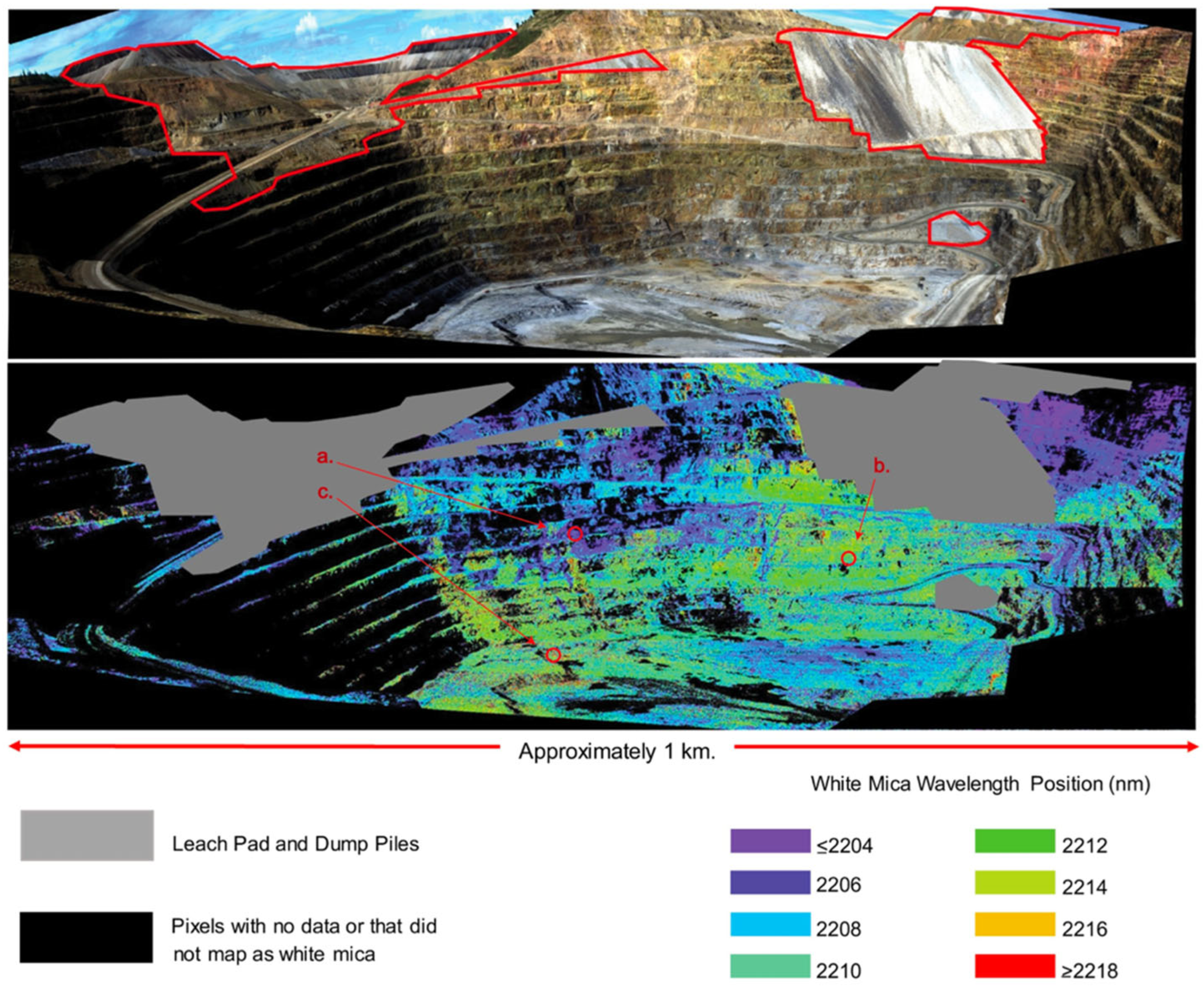
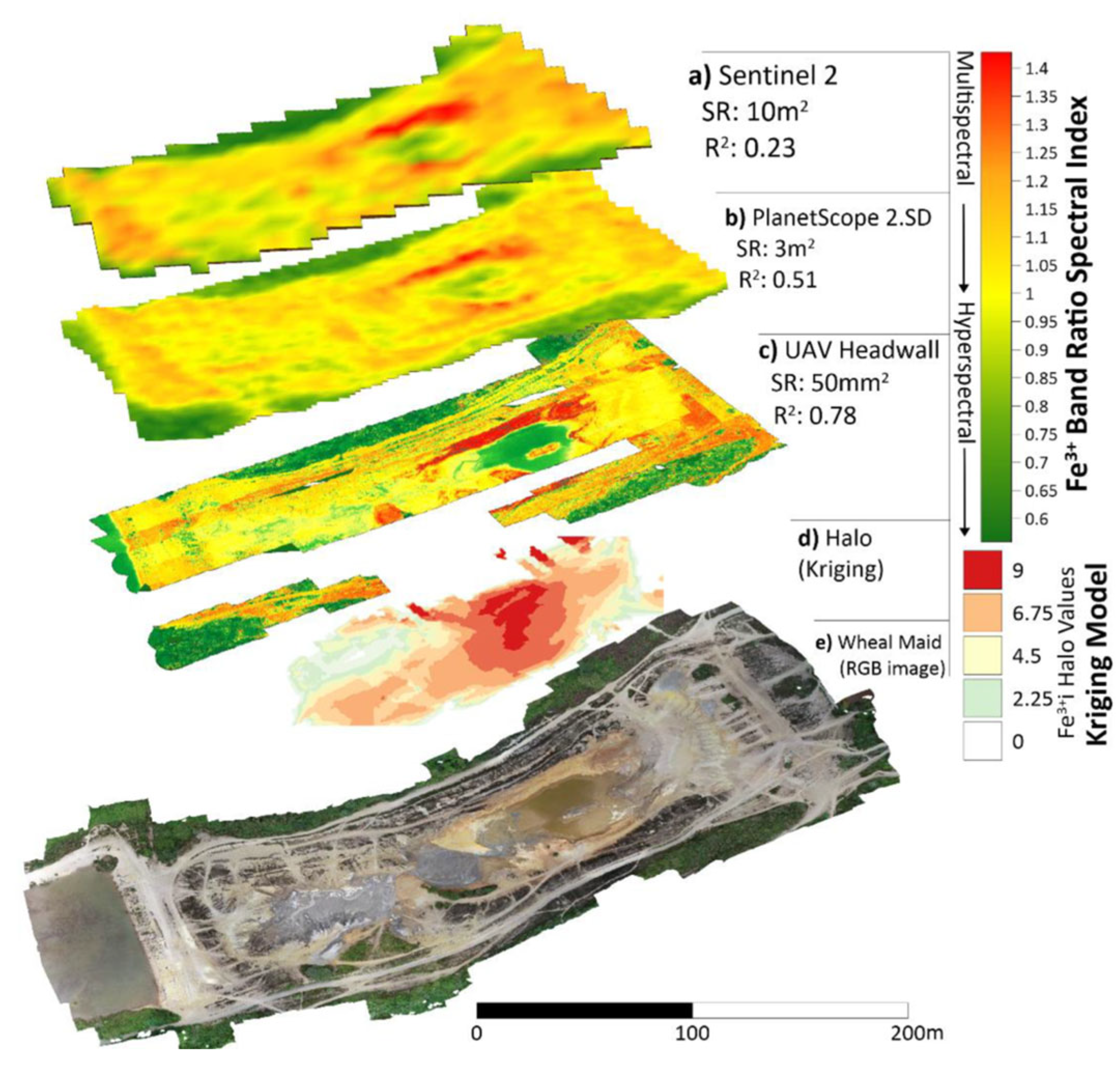
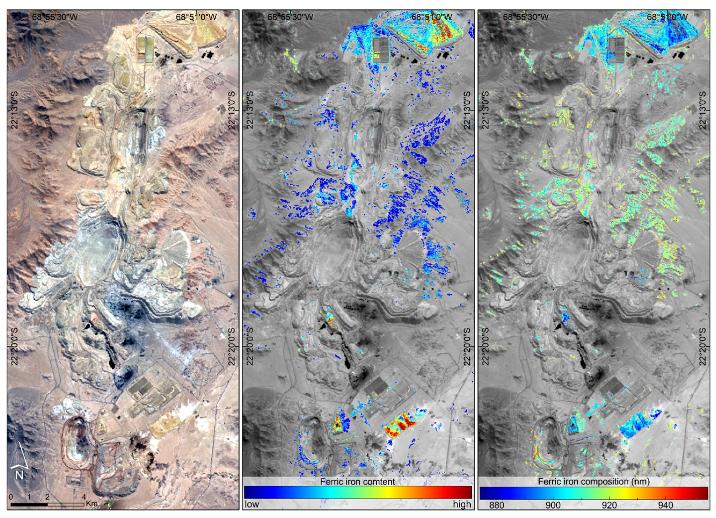
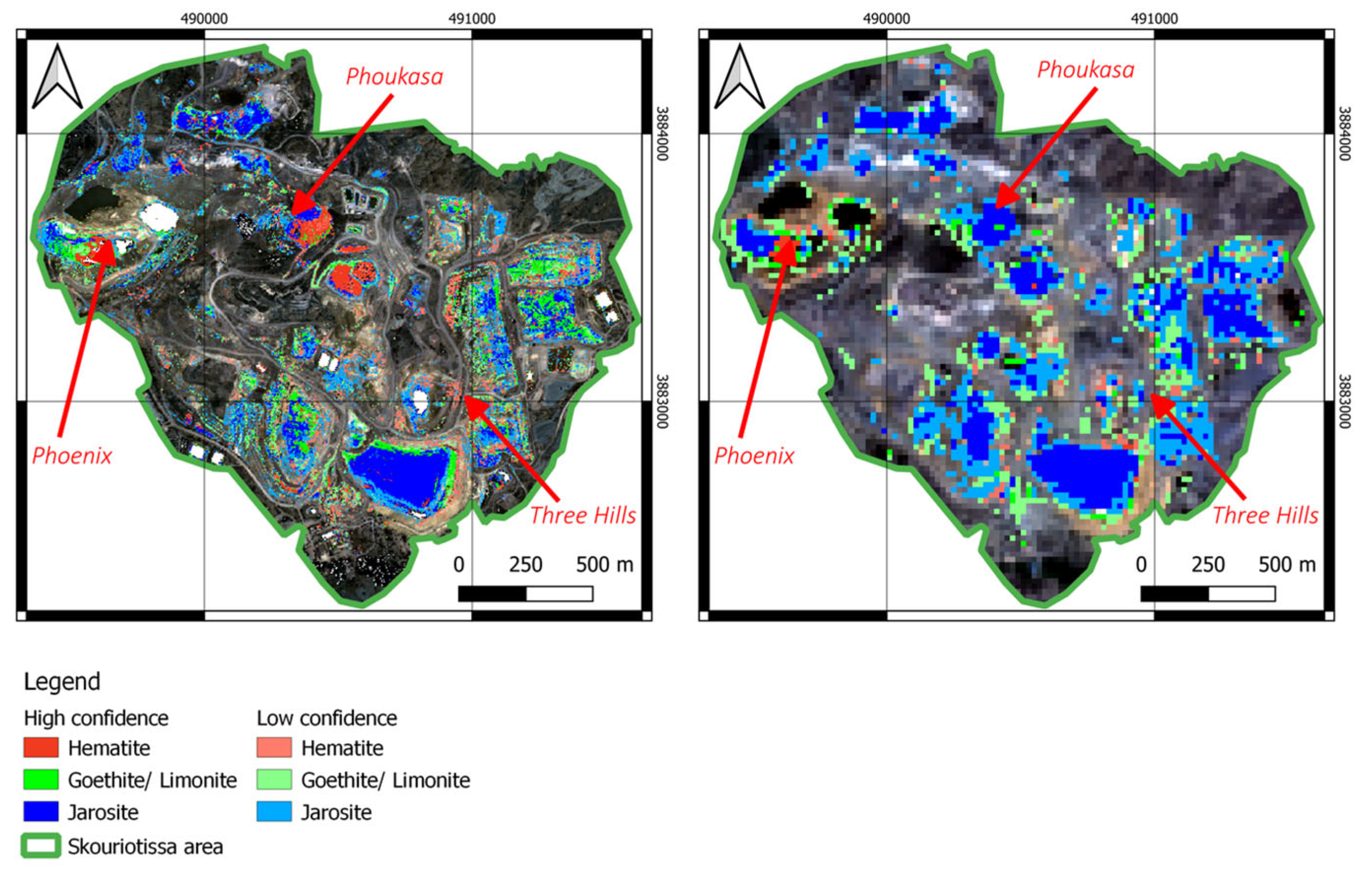
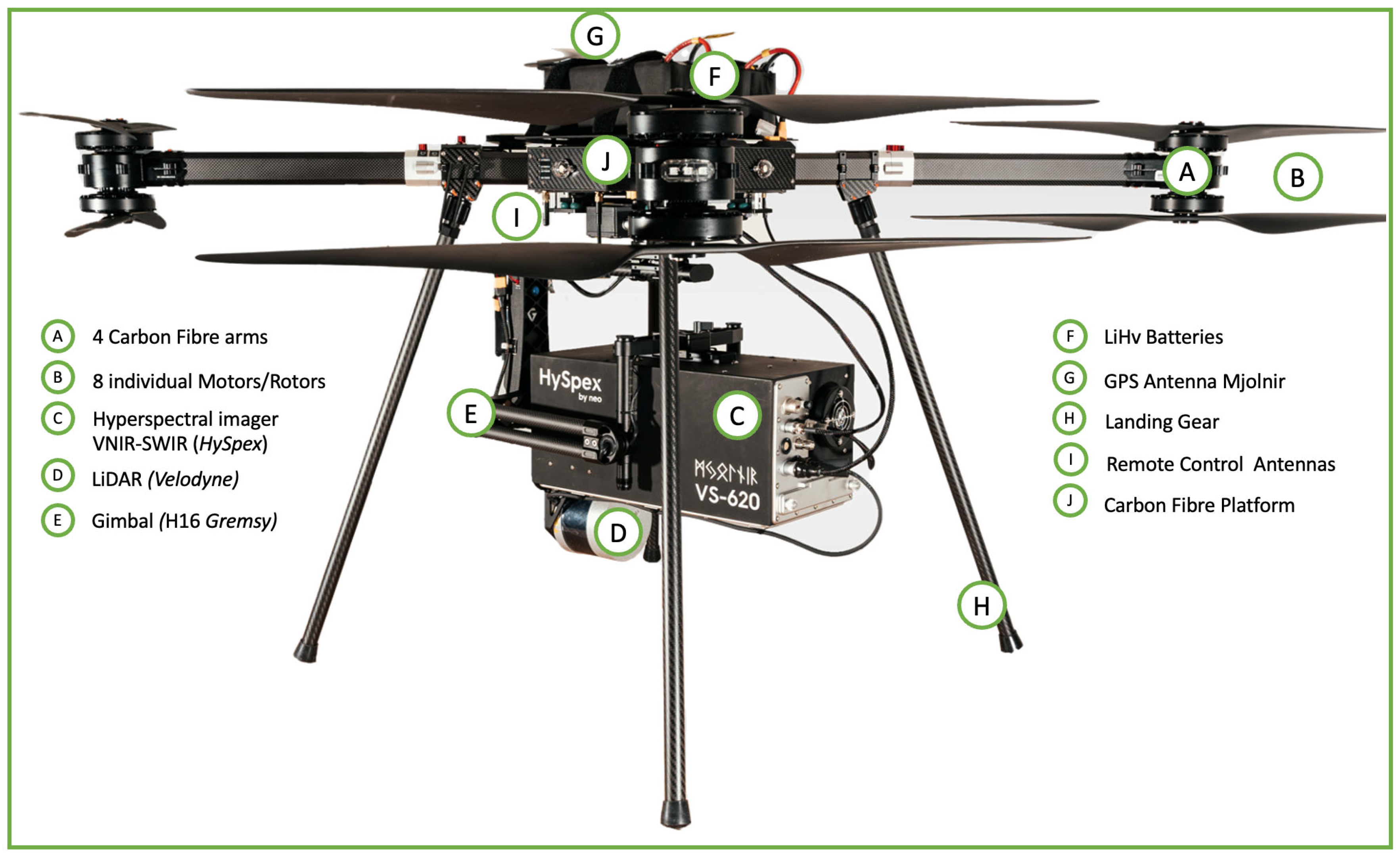
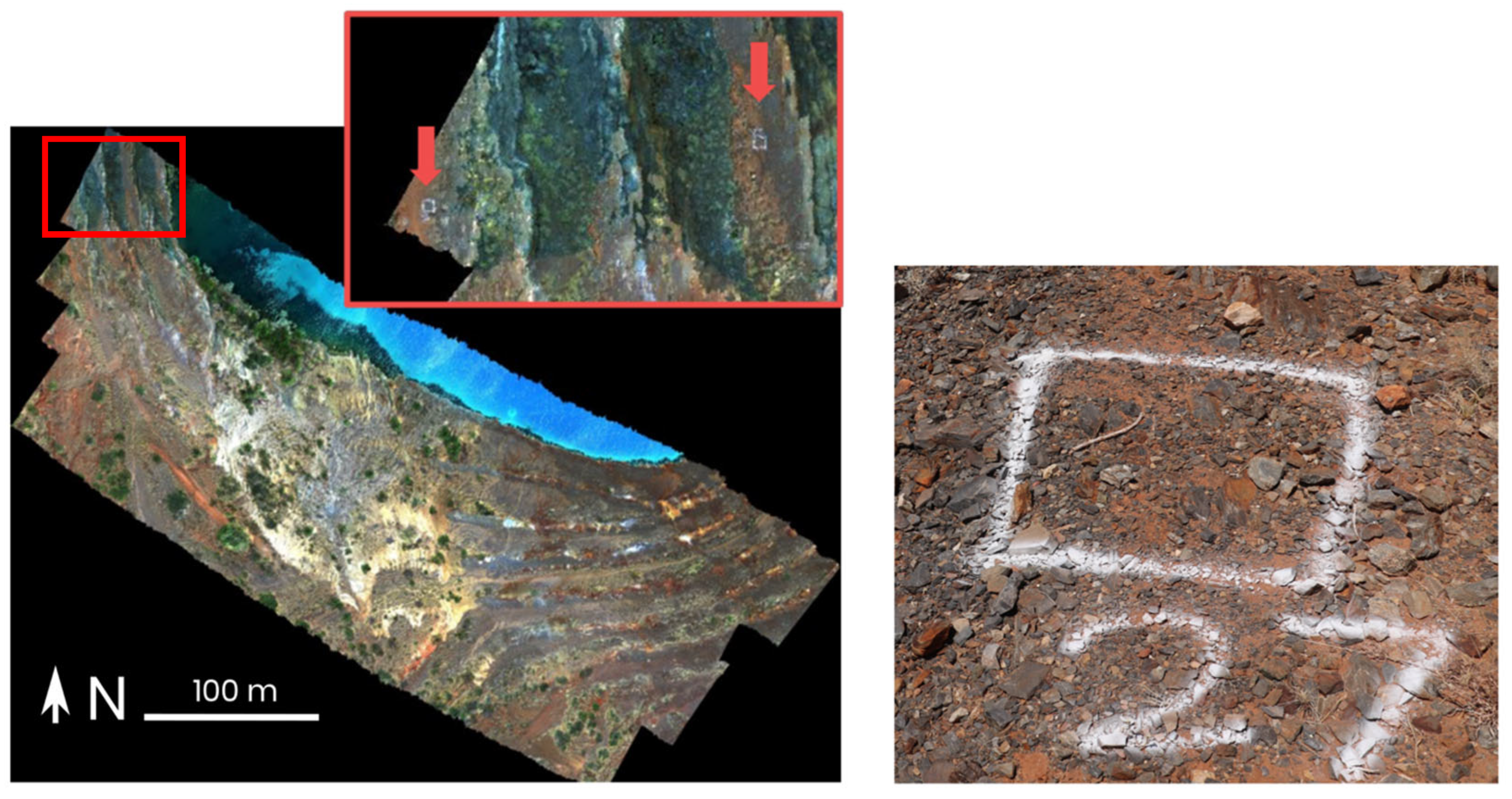
Name (Service Provider/Brand/Name of Instrument)Wavelength RangeType of Data AcquisitionSpectral Bands and SamplingSource (Accessed on DD/MM/YY)
NEO/HySpex
Mjolnir VS-620
VNIR (400–1000 nm)
SWIR (970–2500 nm)
Pushbroom200 bands @ 3 nm;
300 bands @ 5.1 nm
https://www.hyspex.com/hyspex-turnkey-solutions/uav/ (accessed on 1 March 2024)
Headwall Nano HPVNIR (400–1000 nm)340 bands @ 1.76 nmhttps://headwallphotonics.com/products/remote-sensing/nano-hp-400-1000nm-hyperspectral-imaging-package/ (accessed on 1 March 2024)
Headwall Micro 640SWIR (900–2500 nm)267 bands @ 6 nmhttps://headwallphotonics.com/products/remote-sensing/swir-640-900-2500nm-hyperspectral-imaging-package/ (accessed on 1 March 2024)
Headwall Co-Aligned HPVNIR (400–1000 nm)
SWIR (900–2500 nm
340 bands @ 1.76 nm;
267 bands @ 6 nm
https://headwallphotonics.com/products/remote-sensing/co-aligned-hp-400-2500nm-hyperspectral-imaging-package/ (accessed on 1 March 2024)
Specim AFX10VNIR (400–1000 nm)224 bands @ 2.68 nmhttps://www.specim.com/products/specim-afx10/ (accessed on 1 March 2024)
Specim AFX17VIS-NIR (400–1700 nm)224 bands @ 3.5 nmhttps://www.specim.com/products/specim-afx17/ (accessed on 1 March 2024)
Resonon Pika LVNIR (400–1000 nm)281 bands @ 2.7 nmhttps://resonon.com/Pika-L (accessed on 1 March 2024)
Resonon Pika IR-LNIR (925–1700 nm236 bands @ 5.9 nmhttps://resonon.com/Pika-IR-L (accessed on 1 March 2024)
BaySpec OCI-UAVVNIR (600–1000 nm)Pushbroom and snapshot100 bands @ 5 nmhttps://www.bayspec.com/news/bayspec-introduces-ultra-miniaturized-hyperspectral-imager/ (accessed on 1 March 2024)
Senop RikolaVNIR (500–900 nm)Frame-based snapshot50 bands @ 8 nmhttps://senop.fi/optics-imaging/hyperspectral-imaging/ (accessed on 1 March 2024)
Senop HSC-2VNIR (500–900 nm)up to 1000 freely selectable bands @ 6–18 nm,https://senop.fi/optics-imaging/hyperspectral-imaging/ (accessed on 1 March 2024)
Cubert GmbH ULTRIS X20UV-VNIR (350–1000 nm)Snapshot164 bands @ 4 nmhttps://cubert-hyperspectral.com/en/ultris-x20/ (accessed on 1 March 2024)
Telops Hyper-Cam Nano (announced April 2024)VIS–NIR (400–1700 nm)No information availableNo information availablehttps://www.exosens.com/products/high-performance-fast-cameras (accessed on 1 March 2024)
Haip Solutions—Black Bird 2VNIR (500–1000 nm)Hovering Linescanner100 bands @ 5 nmhttps://www.haip-solutions.com/hyperspectral-cameras/hyperspectral-camera-drone/
Disclaimer/Publisher’s Note: The statements, opinions and data contained in all publications are solely those of the individual author(s) and contributor(s) and not of MDPI and/or the editor(s). MDPI and/or the editor(s) disclaim responsibility for any injury to people or property resulting from any ideas, methods, instructions or products referred to in the content.

