1. Introduction
From 1991 to 2023, approximately 125,000 hectares of lignite mining operations in Germany have been renatured. The total land use of lignite mining since its beginnings amounts to around 3000 km
2 [
1]. With the forthcoming phase-out of lignite-fired power generation, significant portions of these areas will be rehabilitated, recultivated, and repurposed for various uses. A substantial portion of these areas comprises the inner dumps of opencast mines. Plans for these repurposed lands include agriculture, forestry, and lakes, as well as infrastructure for traffic and renewable energies (as seen in, e.g., [
2,
3,
4]).
The use of mine dump surfaces, such as for traffic or energy infrastructure construction, often begins before the dump has fully settled. A critical factor in future mine dump development is ground deformation, particularly the settlement behavior of the surface. This behavior is primarily defined by the indicators’ total amount of settlement and the time required for total subsidence to occur.
Settlement effects on open pit dumps can be categorized into self-settlement and load settlement. Load settlements are typically addressed in local geotechnical investigations during detailed construction design and are not the focus of this paper. The self-settlement of open pit dumps primarily results from the dump’s own weight, followed by the weathering and degradation of materials. This process begins immediately after dumping and predominantly occurs in the dewatered section of the dump. The rate of settlement decreases over time until it completely stops. Additional settlement occurs after dewatering measures end, as the resurgence of groundwater in the dump increases the bedding density of the loose rock, leading to sudden settlement effects or slumping [
5]. Moreover, the uplift and compression of the underlying geological layers also influence ground movements observed on the dump’s surface. Uplift is caused by the stress reduction due to the removal of overburden during mining, while compression results from the reloading of the open pit inner dump. This process is considered complete in dump areas sufficiently distant from the open pit [
6].
The self-settlement of open pit dumps has been the subject of research for many decades [
7,
8,
9,
10]. Factors influencing the settlement behavior are, among others, the distance to the slope, the time interval since dumping, the dump design and technology, the soil composition, the groundwater balance, and the relief of the underlying soil. Their complex interaction and the heterogeneity of the material within the dump make it very difficult to implement numerical or analytical solutions for predicting settlement that meet practical requirements. The number of parameters that such types of models require would exceed practicality; statistical inference from available data would make the process rather difficult. Therefore, empirical solutions have prevailed for the prediction of the self-settlement of open pit dumps. These are based on evaluations of in situ measurements, which allow a temporal extrapolation of the settlement behavior (as seen in, e.g., [
11]).
So far, documented evaluations have been largely based on settlement observations at fixed elevation points determined by geodetic leveling. Due to the low spatial density of these geodetic markers, only local statements can be derived. It is not possible to conduct spatial investigations on this basis. Likewise, the observation of settlements is limited to larger time intervals. A more detailed analysis with regard to the influencing factors on the basis of elevation is not possible, or only possible to a very limited extent.
With the development of satellite-based radar interferometry, a monitoring method is available that generates ground motion data that is very dense in area and time. In various applications, e.g., the European project i2Mon, it has been demonstrated that especially the Sentinel 1 sensor, in combination with the SBAS method, can be used for area monitoring on not yet overgrown open pit dumps [
12].
By combining a data-driven approach, using InSAR-generated high-resolution datasets, with model-driven methods such as inverse modeling and classic time–settlement models, the efficient monitoring and prediction of opencast mine dump settlements can be achieved. The question arises as to whether previously mentioned evaluation and forecasting models for subsidence on opencast mine dumps can also be applied to satellite-based radar data. The following question concerns the information potential that this data could provide: Can a large amount of time–settlement information available over a large area in conjunction with statistical/geostatistical evaluation lead to a more detailed forecasting approach? This article will specifically address the first question and demonstrate the potential for answering the second question through a specific case study.
The first part of this contribution presents established methods for predicting settlements. Radar interferometry as a comparatively new observation method is briefly described and its results are characterized with regard to the use for the description of movements on the surface of opencast mine dumps. This is followed by the exemplary application of the presented empirical prediction method to radar interferometric data. A spatial consideration of the results leads to the presentation of the potential of data-driven prediction of settlements in the temporal dimension as well as by transfer to neighboring, unobserved areas. The article concludes with the derivation of further investigation steps.
2. Materials and Methods
2.1. Time–Settlement Function
A reliable description of the time–settlement behavior should be based on the evaluation of in situ measurements on the surface of the dump. For practical reasons, these cannot be carried out starting directly from the time of dumping. Only a partial part of the settlement process over time can be observed. The indicators of practical relevance, i.e., ‘total settlement’ and the ‘time of decay’, should be derived from this by extrapolation. For this purpose, a model has to be established that describes the relation between timely progression and settlement behavior. A model-based description of the temporal settlement behavior
s(
t) has been the subject of different research works. In addition to hyperbolic and logarithmic functions, the approach using the exponential function was well-established in practice (as seen in, e.g., [
10]):
The parameters
smax describe the maximum amount of self-settlement and
c is the time development.
Figure 1 shows such a time–settlement function. It should be noted that the origin of the coordinate system coincides with the start of the observation. The parameter
smax(B) derived from this corresponds to the maximum amount of settlement in relation to the start of the observation. The total settlement
smax results from the sum of
smax(B) and the initial settlement
sA, which occurred between the dumping time and the start of observation. This period is also referred to as the lay time. A time–settlement function derived from the observation data, according to Equation (1), thus practically has the following form:
Based on this equation, the initial settlement
sA can be estimated using
with the lay time
Note that
t0 is a negative value. In the case of several dumping slices, the documented literature (e.g., [
11]) proposes the use of a thickness-weighted average lying time.
2.2. Satellite-Based Radar Interferometry
The method of satellite-based radar interferometry is well established in geomonitoring. For more than a decade, it has been successfully used to detect and characterize ground movements over large areas and in high temporal resolution [
13,
14,
15]. It is very well suited to monitoring large-scale and comparatively slow continuous ground movements and deformation processes in areas of mining. For example, the PSI evaluation of a stack of radar satellite images provides spatially densely arranged time series in high resolution. Detectable movement rates are in the range of 1 mm/a (as seen in, e.g., [
16]). The need for natural and artificial backscatterers makes the application of PSI evaluation particularly suitable for built-up areas with roofs or asphalt surfaces or similar. Rough mining dump surfaces initially seemed less suitable. However, various documented applications [
12,
17] have shown that the use of distributed scatterers (DSs) in combination with the SBAS method can provide reliable data on these surfaces, also using data from the Copernicus Sentinel 1 sensor. In addition, new evaluation methods also offer a higher point density. For example, the SqueeSAR method [
18] not only detects discrete backscatterers (permanent scatterers, PSs) but also distributed scatterers (DSs). By detecting PS and DS, the number of detected elements increases considerably.
These developments make it possible to generate a spatio-temporally high-resolution database of vertical, but also horizontal (limited to east–west direction), ground movement components on opencast mine dumps.
2.3. Parameter Estimation of the Time–Settlement Function Using Minimum Least Squares
The parameters of the time–settlement function are estimated as location-specific from the observed time series for each measurement point using a method of least squares (as seen in, e.g., [
19]). The parameter vector to be estimated contains the observed maximum settlement
smax(B) and the time parameter
c.
According to the method of minimum least squares, this vector can be calculated using
where
A is the deign matrix and
l is the vector of residual observations. The elements of the rows and columns of the design matrix
A can be derived according to
and
The index
i describes the line corresponding to the respective observed value in the time series. The parameters
smax(B)(0) and the time parameter
c(
0) are prior parameters to be estimated, summarized in the vector of prior parameters
x0. The vector of residual observations
l results from the following:
For this purpose, approximate observations L0 are to be calculated using approximation parameter vector x0 applied to Equation (2) and the actual observations L are reduced by these. To determine the final adjusted parameter vector, the result vector x (Equation (6)) has to be added to the prior parameter vector is x0.
The empirical covariance matrix is used to estimate the uncertainty of the estimated parameters. This results from the product of the empirical variance of the residuals
with the cofactor matrix of the adjusted parameters
:
with
and
Here, v is the vector of residuals between measured values and adjusted observations (adjusted model). Equation (11) is valid under the assumption of equally precise observations. The uncertainty of the estimated parameters refers to the elements of the main diagonal of the empirical covariance matrix.
2.4. Derivation of Reference Parameters
Reference parameters are introduced to compare the settlement behavior over time and to achieve the greatest possible general validity. On the one hand, it is recommended to standardize the absolute amount of the total settlement
smax by the thickness of the mine dump
M under consideration. This leads to deformation or relative total settlement [
11]:
Furthermore, a time value is introduced at which the x% of the total settlement or the observed settlement has occurred [
11]. This can be calculated using
Typical values for x are 95% or 99%. Depending on the reference time, the time of dumping or time of the start of observation, refers either to smax or smax(B).
2.5. Practical Considerations
According to [
11], the observation period of measuring points should be at least two years in order to be able to make the time–settlement curve sufficiently robust and thus enable a statistically reliable extrapolation. Furthermore, the location of the measuring points should be considered critically with regard to the position in relation to the crest lines of mine dump slopes and transition areas between natural and tilted subsoil.
Documented case studies comprise observation locations recorded by geometric levelling, which were also measured at comparatively long intervals. In contrast, satellite-based radar interferometry today offers a much more informative database. Ground movement data can be recorded at grid intervals of a few meters. The possibilities arising from this will be examined in the following section. A hypothesis can be formulated as follows:
The time–settlement behavior on opencast mine dumps can be characterized on an a spatially dense basis;
Based on this, locally differentiated and temporally more precise forecasts can be derived with regard to total settlement, residual settlement and the period until the final subsidence on the dump surface occurs;
Linking the areal data with information on geometry and dump structure, composition of the dump from soil groups, dumping technology, etc., allows further correlations to be formulated, which improve the process understanding of the settlement behavior and ultimately also forecast models.
It should be noted that independent of the advantages of InSAR monitoring, a network of geodetic levelling points should be maintained for comparison as a ground truth reference and to ensure reliable results.
3. Results
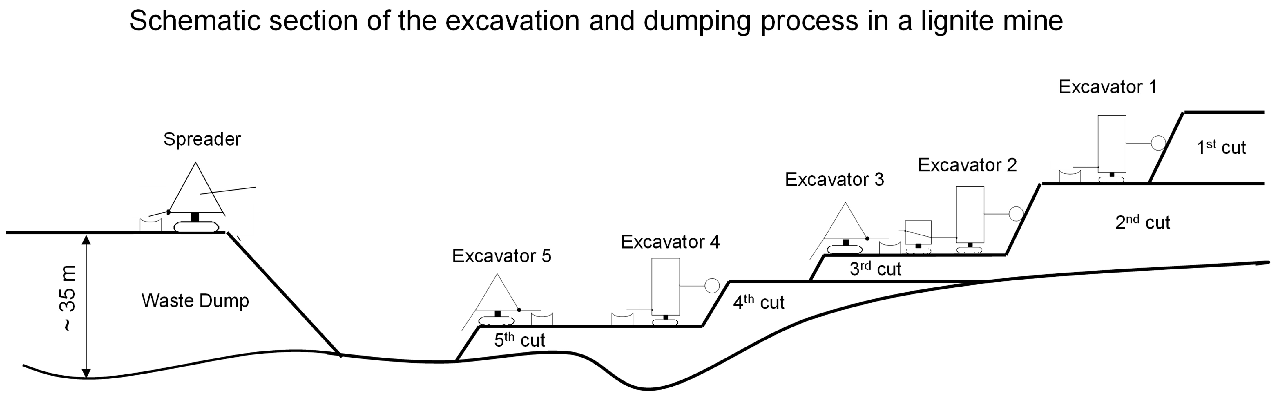
The case study considered is part of an internal dump in central Germany and has an area size of approx. 900 × 900 m. The dumping process by a spreader took place between the years 2013 and 2014.
Figure 2 shows a general cross-section of the geology, as well as the mining and dumping process. The thickness of the dump is on average 35 m. A detailed dump block model, which characterizes the composition of the soil at a resolution of 5 × 5 × 5 m is available. It includes a time stamp of the dumping [
20,
21] and can be used to reconstruct the dumping process over time. In general, the dumped material can be described as mixed soil, which contains different proportions of tertiary sands and clays.
3.1. Dataset
A ground movement monitoring dataset based on satellite-based radar interferometry with a spatial resolution of approx. 15 × 15 m and a temporal resolution of 3 days was used. It covers the period from January 2017 to December 2019. The dataset was generated by Airbus Defence and Space GmbH, Potsdam, for MIBRAG and made available for research purposes as part of the TRIM4PostMining R&D project at the TU Bergakademie Freiberg. All illustrations are based on these data (© Airbus Defence and Space GmbH, Potsdam, Germany).
3.2. Determination of the Time–Settlement Function Parameters
The determination of the parameters is illustrated using a single DS point.
Figure 3 shows the course of the radar interferometric elevation data and the model fitting. The DS point is located in the center of the dump area with a dump thickness of around 35 m. The adjustment of the model is based on data over a period of three years, starting on 1 January 2017. The parameters of the exponential subsidence function were estimated using the least squares method, in accordance with
Section 2.3.
Table 1 summarizes the parameters determined according to the procedure explained in
Section 2.2. When compared to other documented case studies, values derived for deformation and temporal behavior appear plausible.
The application of the presented method to all DS points allows a spatial view of the parameters of the settlement function.
Figure 4,
Figure 5 and
Figure 6 show the spatial distribution of the parameters
smax(
B)
, smax, and
c.
Figure 4 shows the maximum settlement starting from observation derived from the DS data. The values cover a range from 0 mm to −400 mm. The spatial distribution of the values appears plausible. In the west and north, the dump is constructed against grown ground, and the dump thickness increases in these areas towards the south and east. In the south, an area of very high amount of settlement is noticeable.
Figure 5 shows the maximum settlement starting from the dumping time point derived from the DS data. The values cover a range from 0 mm to −900 mm and were derived by taking into account the dumping time from the available dump model. In the central southern area, some DS points with a very high total settlement can be seen, which do not fit into the otherwise rather smooth spatial pattern. These are due to dumping times that deviate from the surrounding area and can be attributed to local locations where earthwork was subsequently performed on the dump. Irrespective of this, the spatial pattern of the settlement behavior seen in
Figure 4 is confirmed.
The spatial distribution of the time factor
c shown in
Figure 6 shows a differentiated behavior compared to the settlement amount. There is no direct correlation to the dump thickness. Areas are recognizable (e.g., the southeastern area) in which settlement occurred more quickly than in other areas. The reason for this could be the different composition of dump material. This needs to be confirmed in a future study.
The spatial distribution of the settlement relative to dump thickness is shown in
Figure 7. The spatial distribution of this parameter indicates the non-random influence of other factors. It can be assumed that, for example, the composition of the dump in terms of soil types, local hydrological characteristics, or the proximity to the top of the slope of the dump (the slope ratio) can affect the deformation locally. The detailed consideration of these factors is not part of this article but is a subject of our ongoing research.
3.3. Prediction of Settlement Behavior Utilizing the Derived Model
To predict the settlement behavior on the dump surface, the presented model with the spatially distributed derived parameters can be used. Two factors need to be distinguished, i.e., timely and spatial prediction. The time forecast aims to predict settlements to be expected in the future at observed locations. The spatial forecast aims to extrapolate the gained knowledge about the settlement behavior to other areas of the dump that have not yet been observed.
Figure 8 shows areas to showcase these aspects. The area marked in yellow corresponds to the area where observations are available. The area marked in green has not yet been observed. For this area, the settlement behavior shall be extrapolated.
3.3.1. Prediction of the Expected Future Settlement Behavior in the Observation Area
With the determined parameters of the time–settlement function derived for each DS point, the process is described not only for the observation period—assuming that the movement behavior does not change significantly, the model can also be used for temporal extrapolation.
The time–settlement function in combination with Equation (14) provides the estimate of the time until a fraction of the total settlement to be defined has decayed. A typical amount is, for example, 95%.
Figure 9 shows this prediction for the observed area. In the eastern part of the dump, the residual settlement time is about 70 to 100 months, which corresponds to about 6 to 8 years. In the western and southern part, the time to decay is 100 to 170 months, which corresponds to about 8 to 14 years.
Other model-based predictions are readily possible, such as a prediction of residual settlement or settlement that has occurred at any point in time, or estimating the time until an absolute amount of residual settlement remains, e.g., 50 mm.
3.3.2. Prediction of the Settlement Behavior Outside the Observation Area
To transfer the results from the observed area of the dump to other areas, the statistical indicators of the estimated parameters can be used. The time coefficient c and deformation ε are suitable for this purpose.
Figure 10 shows the frequency distribution of the deformation characteristics derived from all DS time series. The arithmetic mean of the deformation is 0.96% with a standard deviation of ±36%. Without any additional information and assuming that the dumping technology and composition of the dumping material do not change significantly, the mean value can be transferred to neighboring areas. This makes it possible to make a sufficiently good prediction with the uncertainty range of the standard deviation.
Figure 11 presents the frequency distribution of the time coefficient c. With a mean value of −0.03 1/month and a standard deviation of ±0.004 1/month, this coefficient shows little variation. This information can also be transferred to technologically comparable areas of the dump.
A more sophisticated approach is spatial extrapolation using, for example, simple kriging (as seen in, e.g., [
22]). To describe the spatial structure, a variogram has to be modelled using the spatially distributed parameters at DS locations. The application of a kriging operator on parameter deformation and the time coefficient for interpolation on a grid covering the area of spatial prediction allows us to describe spatial settlement behavior.
Figure 12 shows the example of the derived estimated maximum settlement
smax. In addition, the kriging operator enables the estimation of the variance describing the uncertainty of the settlement prediction, as shown in
Figure 13. The square root of the estimation variance is a standard deviation and can be used as an uncertainty interval.
3.4. Accuracy Considerations
3.4.1. Quality of the Model Fit
To assess the goodness of fit of the model for the observed data, the coefficient of determination
B was used (as seen in, e.g., [
19]).
This coefficient describes the proportion of the variance of the data that is explained by the model. With a value of
B = 0.97 for the DS point shown in
Figure 3, the model can be rated as a very good fit. The differences between the model and the observed value (residuals) are shown for the DS point considered in
Figure 14.
Table 2 summarizes the statistics of the residuals. Regarding the order of magnitude of the values presented in
Table 2, it can be seen that the deviations are negligible in terms of practical issues.
It is noticeable that the deviations shown in
Figure 14 are not purely random, but show a temporal autocorrelation. These phenomena can be explained by temporary influences of the InSAR data, e.g., by atmospheric processes (as seen in [
13]), as well as by the settlements themselves. The latter could be, for example, uplift phenomena caused by meteoric phenomena such as freezing or accelerated settlement phenomena caused by the infiltration of prolonged precipitation into the dump surface. Even if the explanation of these phenomena seems to be scientifically interesting, it is of no practical importance due to the very small amounts of movement and shall not be considered further here.
With an observation period of at least two to three years, as discussed in
Section 2.5, these effects can be filtered out and representative settlement model can be estimated. A discussion on the remaining uncertainty follows next.
3.4.2. Uncertainties in the Prognosis
Based on the results of the adjustment of observations, the uncertainties in the estimated parameters “total settlement”,
, and “time coefficient”,
, can be determined. For this purpose, the standard deviation of the adjusted parameters is used. These can be directly derived from the empirical covariance matrix (Equation (10)). If these uncertainties are related to the absolute value of the maximum settling and the time coefficient per observation point, the relative error is obtained.
Figure 15 and
Figure 16 show these in the observed area. For the maximum settlement, relative errors of 0.0% to 15.0% can be seen. For the time coefficient, the relative error ranges from between 0.0% and 3.5%.
The application of the law of error propagation law allows an estimation of the uncertainty of the settlement at any point in time
.
Formula (16), applied to an observed DS point, provides information about the uncertainty of the prognosis of the future settlement history at that location. With good model fit, this uncertainty is comparatively small.
Figure 16 shows in the left part the predicted course and the uncertainty for the previously discussed DS point. If Formula (16) is applied to areas of the dump area which have not been observed, the uncertainties take the values mentioned in
Section 3.3.2 for
smax = (0.96% ± 0.34%) × M and c = (−0.03 ± 0.004) 1/month. The right graph in
Figure 17 represents this case scenario. It should be emphasized that this uncertainty is very conservative and applies to areas which are far away from the observation points.
4. Discussion
Satellite-based radar interferometry provides highly detailed spatio-temporal ground motion data across large areas, which is particularly suited for monitoring open-pit mining dumps. When integrated with classical time–settlement models, these data reveal a strong fit, enabling the precise modeling of the self-settlement process in such dumps. Parameter estimation for time–settlement curves was implemented using the least squares method, which was coded in Python for this study [
23]. This method yields spatially dense time–settlement models, allowing the accurate prediction of settlement behavior. The predictions are largely data-driven, requiring minimal knowledge of the dump’s internal structure. Consequently, future settlements in observed dump areas can be forecast with high accuracy.
Moreover, these findings on settlement behavior can be extended to unobserved dump areas, within defined accuracy limits. This extrapolation assumes stationarity, meaning that the subsidence process remains spatially and temporally consistent within the system boundaries. Specifically, it assumes that the dump’s geological composition and the overall behavior of the settlement process do not significantly change. For spatially constrained lignite mines situated in a broader regional geological context, this assumption may hold but should be critically evaluated for each specific case.
Radar interferometry not only elucidates the spatial patterns of subsidence but also generates a comprehensive dataset for further exploration. Potential future studies could explore links between settlement behavior and factors such as dumping technology, geometric configuration, and material composition. Incorporating these factors into the models could improve predictions in unobserved areas.
Although the method demonstrated here applies to one specific case study, it can be generalized to model undisturbed settlement processes. However, when additional factors such as rising groundwater influence settlement behavior, alternative models, such as those accounting for slumping, should be considered to ensure accuracy.
5. Conclusions
This contribution presents an inverse modeling approach that utilizes the high spatio-temporal resolution of InSAR data for ground movement monitoring, enabling the data-driven predictions of settlement in waste dumps. The method was applied to a case study in central Germany, demonstrating that the settlement process can be effectively modeled, allowing both temporal and spatial predictions. Leveraging freely available Sentinel 1 data and their wide spatial coverage makes the method highly cost-efficient. It can also be executed without direct access to the dump site. With a spatial resolution of approximately 15 × 15 m, the approach provides relatively dense information. If higher spatial resolution is needed, alternative sensors like TerraSAR-X should be considered.
This method has certain limitations, such as the assumption of stationarity—requiring that the time–settlement process remains undisturbed—and that the geological composition of the waste dump remains generally unchanged. Additionally, the independent validation of InSAR results is necessary, with geodetic leveling required as a ground-truth reference.
This method could potentially be generalized to other mine dumps without significant adjustments. Moreover, it may be applicable to slope monitoring, particularly for slopes following an east–west (EW) direction, given InSAR’s limitation in detecting horizontal ground movements.
Author Contributions
Conceptualization, J.B. and N.M.; methodology, N.M.; software, J.B. and A.J.; formal analysis, N.M.; investigation, N.M.; writing—original draft preparation, N.M. and J.B.; writing—review and editing, J.B.; visualization, A.J.; supervision, J.B.; project administration, J.B.; funding acquisition, J.B. All authors have read and agreed to the published version of the manuscript.
Funding
The article was produced as part of the H2020—RFCS-funded project TRIM4PostMINING. The project received funding under a grant agreement.
Data Availability Statement
Data are not available publicly due to confidentiality reasons.
Conflicts of Interest
Author Natalie Merkel was employed by the company KODIAK GmbH. The remaining authors declare that the research was conducted in the absence of any commercial or financial relationships that could be construed as a potential conflict of interest.
References
- Statista Research Department. Braunkohlenbergbau: Rekultivierte Flächen nach Nutzungsart in Deutschland bis 2021. 2021. Available online: https://de.statista.com/statistik/daten/studie/184752/umfrage/braunkohlenbergbau-wieder-nutzbar-gemachte-flaechen-in-deutschland/ (accessed on 28 December 2022).
- Galiläer, P.; Bennewitz, T. Construction of interstate highways on mining dumps in the south of Leipzig. Straße Autob. 2008, 7, 394–402. (In German) [Google Scholar]
- Schröder, C.; Bürgl, K.; Annanias, Y.; Niekler, A.; Müller, L.; Wiegreffe, D.; Bender, C.; Mengs, C.; Scheuermann, G.; Heyer, G. Supporting land reuse of former open pit mining sites using text classification and active learning. arXiv 2021, arXiv:2105.05557. [Google Scholar]
- Geß, S. Construction on mining dumps—A challange with respect to geotechnical safety. In Proceedings of the 17. Tagung für Ingenieurgeologie und Forum Junge Ingenieurgeologen in Zittau, Zittau, Germany, 6–9 May 2009. (In German). [Google Scholar]
- Koner, R.; Chakravarty, D. Characterisation of overburden dump materials: A case study from the Wardha valley coal field. Bull. Eng. Geol. Environ. 2016, 75, 1311–1323. [Google Scholar] [CrossRef]
- Fenk, J. Effects on Stress Reductions in Subsurfce Soil. In Markscheidewesen; Deutscher Markscheider-Verein (DMV) e.V.; Springer: Peine, Germany, 2004 (2011); Volume 111, pp. 49–52. (In German) [Google Scholar]
- Dorschner, E. Settlement on Open Cast Dumps in Lignite Mines; Bergakademie Freiberg: Freiberg, Germany, 1965. (In German) [Google Scholar]
- Kothen, H.; Knufinke, H. Residual Settlement on Reclaimed Areas. Bankole 1990, 10, 24–29. (In German) [Google Scholar]
- Nehring, H. Monitoring on mine dump settlements in the rheinish lignite area. Braunkohle Wärme Energ. 1968, 20, 83–91. [Google Scholar]
- Toth, F. Investigation on the Sump Settlement Model in the Hambach Mine; Department of Mine Surveying and Geodesy, TU Bergakademie Freiberg: Freiberg, Germany, 2024; unpublished. [Google Scholar]
- Hallbauer, C. Geotechnical Principles for the Construction of Railroad Lines on Opencast Mine Dumps of Lignite Mining with Special Consideration of the Inherent Settlement Behavior; Fakultät für Technik und Naturwissenschaften, der Hochschule für Verkehrswesen, Friedrich List Dresden: Dresden, Germany, 1981; unpublished. [Google Scholar]
- Yang, C.H.; Stemmler, C.; Pakzad, K.; Zimmermann, K.; Müterthies, A. Integrated Mining Impact Monitoring (Eu-Project I 2 Mon) for Open-Pit and Underground Mines. Int. Arch. Photogramm. Remote Sens. Spat. Inf. Sci. 2022, 43, 367–372. [Google Scholar] [CrossRef]
- Hanssen, R.F. Radar Interferometry: Data Interpretation and Error Analysis; Kluwer Academic Publishers: Dordrecht, Germany, 2001; p. 328. ISBN 0-7923-6945-9. [Google Scholar]
- Wegmuller, U.; Walter, D.; Spreckels, V.; Werner, C.L. Nonuniform ground motion monitoring with TerraSAR-X persistent scatterer interferometry. IEEE Trans. Geosci. Remote Sens. 2009, 48, 895–904. [Google Scholar] [CrossRef]
- Grzempowski, P.; Badura, J.; Milczarek, W.; Blachowski, J.; Głowacki, T.; Zając, M. Determination of the Long-Term Ground Surface Displacements Using a PSI Technique—Case Study on Wrocław (Poland). Appl. Sci. 2020, 10, 3343. [Google Scholar] [CrossRef]
- John, A. Monitoring of Ground Movements Due to Mine Water Rise Using Satellite-Based Radar Interferometry—A Comprehensive Case Study for Low Movement Rates in the German Mining Area Lugau/Oelsnitz. Mining 2021, 1, 35–58. [Google Scholar] [CrossRef]
- Nádudvari, Á. Using radar interferometry and SBAS technique to detect surface subsidence relating to coal mining in Upper Silesia from 1993–2000 and 2003–2010. Environ. Socio-Econ. Stud. 2016, 4, 24–34. [Google Scholar] [CrossRef]
- Ferretti, A.; Fumagalli, A.; Novali, F.; Prati, C.; Rocca, F.; Rucci, A. A new algorithm for processing interferometric data-stacks: SqueeSAR. IEEE Trans. Geosci. Remote. Sens. 2011, 49, 3460–3470. [Google Scholar] [CrossRef]
- Niemeier, W. Adjustment of Observations—Methods for Statistical Analysis. In Ausgleichungsrechnung; Walter de Gruyter GmbH: Berlin, Germany, 2008. [Google Scholar] [CrossRef]
- Knipfer, A.; Kreßner, M. Results of the Validation Study for Geotechnical Stability Modelling Using the MIBRAG Dump Model. In Proceedings of the Altbergbaukolloquium 2022, TU Bergakademie Freiberg, Freiberg, Germany, 4–5 November 2022. [Google Scholar]
- Benndorf, J.; Restrepo, D.A.; Merkel, N.; John, A.; Buxton, M.; Guatame-Garcia, A.; Dalm, M.; de Waard, B.; Flores, H.; Möllerherm, S.; et al. TRIM4Post-Mining: Transition Information Modelling for Attractive Post-Mining Landscapes—A Conceptual Framework. Mining 2022, 2, 248–277. [Google Scholar] [CrossRef]
- Goovaerts, P. Geostatistics for Natural Resources Evaluation; Oxford University Press: Oxford, UK, 1997. [Google Scholar]
- Van Rossum, G.; Drake, F.L. Python 3 Reference Manual; CreateSpace: Scotts Valley, CA, USA, 2009. [Google Scholar]
Figure 1.
Exponential time–settlement function to characterize temporal self-settlement behavior.
Figure 1.
Exponential time–settlement function to characterize temporal self-settlement behavior.
Figure 2.
General cross-section of the case study showing the general geology and the mining technology on the left side and the dump on the right side (adapted from MIBRAG mbH).
Figure 2.
General cross-section of the case study showing the general geology and the mining technology on the left side and the dump on the right side (adapted from MIBRAG mbH).
Figure 3.
Fitting a settlement function (blue line) to radar data (orange line)(© Airbus Defence and Space GmbH, Germany).
Figure 3.
Fitting a settlement function (blue line) to radar data (orange line)(© Airbus Defence and Space GmbH, Germany).
Figure 4.
Spatial distribution of the parameter ‘maximum amount of settlement’, in accordance with the time of observation start smax(B) derived from the DS series.
Figure 4.
Spatial distribution of the parameter ‘maximum amount of settlement’, in accordance with the time of observation start smax(B) derived from the DS series.
Figure 5.
Spatial distribution of the parameter maximum amount of settlement according to the time of dumping, smax, derived from the DS series.
Figure 5.
Spatial distribution of the parameter maximum amount of settlement according to the time of dumping, smax, derived from the DS series.
Figure 6.
Spatial distribution of the time parameter c of the time–settlement function derived from the DS series.
Figure 6.
Spatial distribution of the time parameter c of the time–settlement function derived from the DS series.
Figure 7.
The spatial distribution of the deformation (maximum amount of settlement relative to dump thickness) in the studied area.
Figure 7.
The spatial distribution of the deformation (maximum amount of settlement relative to dump thickness) in the studied area.
Figure 8.
Definition of the areas of time and spatial prediction in the case study.
Figure 8.
Definition of the areas of time and spatial prediction in the case study.
Figure 9.
Time to reach 95% of total settlement.
Figure 9.
Time to reach 95% of total settlement.
Figure 10.
Frequency distribution of the parameter deformation per DS point in the studied area.
Figure 10.
Frequency distribution of the parameter deformation per DS point in the studied area.
Figure 11.
Frequency distribution of the parameter time coefficient per DS point in the studied area.
Figure 11.
Frequency distribution of the parameter time coefficient per DS point in the studied area.
Figure 12.
Prediction of the maximum settlement in a non-observed area.
Figure 12.
Prediction of the maximum settlement in a non-observed area.
Figure 13.
Uncertainty in the estimated maximum settlement.
Figure 13.
Uncertainty in the estimated maximum settlement.
Figure 14.
Residuals between model and observations for the selected DS point.
Figure 14.
Residuals between model and observations for the selected DS point.
Figure 15.
Areal distribution of the relative error of the total settlement.
Figure 15.
Areal distribution of the relative error of the total settlement.
Figure 16.
Areal distribution of the relative error of the time coefficient.
Figure 16.
Areal distribution of the relative error of the time coefficient.
Figure 17.
Predicted time–settlement curves as solid blue lines with uncertainty band (standard deviation) as dashed lines in green (lower limit) and gray (upper limit) for an observed DS point (left) and an unobserved point on the dump (right).
Figure 17.
Predicted time–settlement curves as solid blue lines with uncertainty band (standard deviation) as dashed lines in green (lower limit) and gray (upper limit) for an observed DS point (left) and an unobserved point on the dump (right).
Table 1.
Summary of the comparison parameters determined for the considered DS point.
Table 1.
Summary of the comparison parameters determined for the considered DS point.
| | Smax(B) in mm | Time of Dumping | SA in mm | Smax in mm | Thickness in m | in % | c in
1/day | t95 in months |
|---|
| DS point | 102 | 18 February 2014 | 194 | 296 | 35 | 0.86 | 0.0010 | 99 |
Table 2.
Deviations between the model and observations in mm.
Table 2.
Deviations between the model and observations in mm.
| | Minimum | Maximum | Mean | Standard Deviation |
|---|
| DS Point | −3.7 | 3.3 | −0.3 | 1.2 |
| Disclaimer/Publisher’s Note: The statements, opinions and data contained in all publications are solely those of the individual author(s) and contributor(s) and not of MDPI and/or the editor(s). MDPI and/or the editor(s) disclaim responsibility for any injury to people or property resulting from any ideas, methods, instructions or products referred to in the content. |
© 2024 by the authors. Licensee MDPI, Basel, Switzerland. This article is an open access article distributed under the terms and conditions of the Creative Commons Attribution (CC BY) license (https://creativecommons.org/licenses/by/4.0/).


