Environmental and Work Factors That Drive Fatigue of Individual Haul Truck Drivers

Abstract

Many factors influence the fatigue state of human beings, and fatigue has a significant adverse effect on the health and safety of the haulage operators in the mine. Among various fatigue monitoring systems in mine operations, currently, the Percentage of Eye Closure (PERCLOS) is common. However, work and other environmental factors influence the fatigue state of haul truck drivers; PERCLOS systems do not consider these factors in their modeling of fatigue. Therefore, modeling work and environmental factors’ impact on individual operations fatigue state could yield interesting insights into managing fatigue. This study provides an approach of using operational data sets to find the leading indicators of the operators’ fatigue. A machine learning algorithm is used to model the fatigue of the individual. eXtreme Gradient Boosting (XGBoost) algorithm is chosen for this model because of its efficiency, accuracy, and feasibility, which integrates multiple tree models and has stronger interpretability. A significant number of negative and positive samples are created from the available data to increase the number of datasets. Then, the results are compared with other existing models. A selected algorithm, along with a big data set was able to create a comprehensive model. The model was able to find the importance of the individual factors along with work and environmental factors among operational data sets.

1. Introduction

Fatigue is an occupational hazard and can be attributed to the health and safety of the worker. It affects the health and safety of both the employees and their colleagues adversely. Fatigue is a complex phenomenon that can be associated with many factors. Fatigue can be defined as a state of feeling tired, weary, or sleepy that results from prolonged physical or mental work, extended periods of anxiety, exposure to harsh environments, or lack of sleep [1]. Fatigue varies from weakened function of alertness during tasks to drowsiness, micro-sleep or completely falling asleep. It can affect worker performance and impair their mental alertness, which can cause dangerous errors [1]. Fatigue presents several challenges for the mining industry. Various accidents have been reported at mine operations, which could be associated with the loss of control due to the fatigue and sleepiness of mineworkers [2]. The mining industry is certainly not alone in facing the challenge of addressing worker fatigue. In fact, many of the characteristics of fatigue in the mining industry mirror the similarities of fatigue in other industries. Hence, any fatigue management applications, training, or interventions from other industries can be borrowed and applied to mining. However, some have argued that mining, in particular, is especially susceptible to increases in the presence of fatigue due to the multifaceted combination of factors in mining environments associated with fatigue: dim lighting; limited visual acuity; hot temperatures; loud noise; highly repetitive, sustained, and monotonous tasks; shiftwork; long work hours; long commute times due to mine site remoteness; early morning awakenings; and generally poor sleep habits [3]. Although the full burden of fatigue on mineworkers has not yet been measured, some technologies can monitor operator fatigue, such as the video-based technology, percentage of eyelid closure over the pupil over time (PERCLOS) system, and Electroencephalography (EEG) cap. While such technologies can detect the fatigue of the operator, they do not necessarily prevent or mitigate fatigue from happening [3]. These technologies have their pros and cons. Video-based technology (PERCLOS) uses eyelid closure as the main measure to detect driver fatigue. However, it has some drawbacks that limit its success, such as darkness limitations and practical hurdles like the distraction of the drivers [4]. On the other hand, the EEG cap uses electrodes to get the signal from the brain and translate it to the status of the driver fatigue. These electrodes and caps have been shown to cause discomfort for drivers, limiting their widespread adoption [5]. Therefore, they are not suitable for long-term monitoring. There is another technology called WOMBATT (Worldwide Online Monitoring By Alerting Tired Travelers), can determine a person’s level of fatigue by analyzing a recording voice [6]. PERCLOS, EEG, WOMBATT and other technologies can detect fatigue, but they cannot recognize factors that affect fatigue such as work-demand factors.

The Job Demand-Resources model (JDR) of worker stress and health shows that too much job demand and not enough resources can result in injuries due to physiological and physical costs [3]. The core part of the JDR model is related to risk factors associated with job stress. These factors can be classified into two general categories, job demands and job resources [7,8,9]. Job demands refer to the physical, psychological, social, or organizational aspects of the job that require physical and psychological effort or skills. However, job demands are not necessarily negative; they may turn into job stressors when those demands require high effort from the employee, which is hard to recover [7]. Job resources refer to the physical, psychological, social, or organizational aspects of the job that are functional in achieving work goals, decreasing job demands, or stimulating personal growth, learning, and development [7,8,9].

2. Previous Studies

Fitness for duty in mining is an important issue which is affected by individual’s physical and psychological fitness. Fatigue is one of the driver of fitness for duty in mining, which greatly is caused by excessive work hours and shiftwork [10,11]. Fatigue in the workplace often results in a reduction in worker performance. Fatigue must be controlled and managed since it causes significant short-term and long-term risks [12,13,14,15]. Other than the health and safety consequences on workers, fatigue can result in damage or loss of valuable mine equipment like haul trucks. So, the mining industry measures operational risk losses to estimate capital allocation and manage operational risks [16,17].

Drews et al. (2020) studied fatigue in the mining industry and mentioned that fatigue in the mining industry is different from other industries because of the specific environmental factors in the mining industry [18]. They also provided some other factors that drive fatigue like repetitive and monotonous tasks, long work hours, shiftwork, sleep deprivation, dim lighting, limited visual acuity, hot temperatures, and loud noise [18]. Multiple psychological and physiological issues impacted the fatigue of the workers, which makes fatigue management difficult. Some technologies can monitor drivers’ fatigue, such as tracking eye movement and head orientation (PERCLOS) or hard hats with electroencephalogram (EEG) activity tracking, with their pros and cons. However, considering these technologies, other studies show that there is no obvious approach to control and mitigate the fatigue of workers in mine operations [3].

Machine learning (ML) can be used to predict leading indicators and help management make appropriate decisions [19,20]. ML is flexible to operate without any statistical assumptions. It also is able to identify any relationships within the phenomena and issues [19,21,22]. Previous study offers that finding leading indicators to predict fatigue in the mining industry can be useful [18]. Due to the complexity of fatigue, using machine learning (ML) algorithms on the real-time data captured from the existed technologies can be helpful to model fatigue. Such a model could identify predictive elements of workers’ fatigue. Some studies are done with the collected data to predict fatigue [18]. However, a comprehensive study using a wider range of available data sets can find more possible independent variables in the model to find top predictive factors. If these factors can be used as fatigue predictive elements, they will enhance safety and health decisions in an earlier time in the fatigue cycle.

In an earlier study done by E. Talebi et al. (2021), machine learning (ML) models were created using aggregated operational data sets from a mine [23]. The findings of that study confirm that fatigue is caused by a wide variety of factors, which are very difficult to quantify. Fatigue prediction is a matter of predicting the complex interactions between human behavior and the changing work environments at mine operations [23]. The model outcome had a low R² value that captures relationships that quantify a relatively high amount of variance in a complex relationship. This high amount of variance is likely largely due to the difficulty of generalizing a model that can predict fatigue due to the complex psychological and physiological factors associated with fatigue at the group level. Only operational data and weather data are utilized in these models aggregated at the mine level [23].

The machine learning model selected for that analysis was a random forest (RF) regression algorithm. This algorithm was chosen because it can be applied well to a wide variety of problems with a rapid speed of training. This analytical tool shows what features of the model have higher effects on the predictions of the model and estimates how marginal changes in those features impact these predicted outcomes [23].

The model output identifies the variables that have the highest impact on all fatigue events. The previous model results offer some interesting insights into the factors that potentially cause fatigue. It shows that while it is not surprising that shift type (night or day) causes fatigue, it is interesting that maintenance processes such as unscheduled downtime and production rates, as well as other operational variables, can affect fatigue among haul truck drivers. Having identified these additional predictors for fatigue, these indicators can be used by managers to prioritize safety management efforts. However, this model was aggregated and averaged out at the mine level. Would a model at a lower level of granularity, say, at the individual level, rather than aggregated at the mine level yield better results? This was the primary difference and guiding research question for the model presented in this paper.

XGBoost algorithm is applied to data to model fatigue. This algorithm is used because it has more power to handle complicated relations. XGBoost is a powerful machine learning (ML) algorithm that has shown strong power to pick up patterns in the data and automatically tune learnable parameters. What is novel in this study compared to the previous study is a higher score of the model to predict fatigue.

3. Case Study

3.1. Data Description

This study used approximately four years of data from a single, large, operating surface mine.

Table 1. Data sets details.

Data Source	Key Factors	Date Range
Fatigue monitoring	Micro-sleeps (low and critical fatigue)	2016–2020
Time and attendance	Hours worked, overtime, etc.	2016–2020
Fleet management system (production and status)	Production cycles, down equipment, delayed equipment, etc.	2016–2020

shows a brief overview of the data sets that were used for modeling fatigue with details of the types of information and the range of dates. The site utilized a PERCLOS monitoring system, which used cameras to track and monitor the eye movements of haul truck drivers to model and detect fatigue. When the camera detected certain eye movements, eye closure, or blinking, the PERCLOS system can determine fatigue based on a preset model. In a situation when the eyes were closed for more than 3 s, the system alerted operators, supervisors, and dispatchers for more action. Data captured from the system was categorized based on the type of event. If the event was a micro-sleep, which was an actual fatigue event, it would be categorized as a low or critical fatigue event. Previous studies by the authors showed that fatigue events captured by fatigue monitoring systems are important indicators of fatigue [10]. Therefore, micro-sleep data was used to model fatigue for this study.

More details of fatigue events are shown in

Table 2. Count and percentage of fatigue event by type.

Fatigue Event Review Type	Number of Fatigue Events	Percentage of Fatigue
Low Fatigue	741	69%
Critical Fatigue	332	31%

. This table demonstrates the number of events by type of fatigue events and the percentage of these fatigue events for comparison. The data shows more low fatigue compared to critical fatigue, representing 69% of the fatigue events that were captured by the system. All fatigue events are reviewed after recording from the fatigue monitoring system, and critical fatigue events are the ones when operators have micro-sleep, while low fatigue events are the ones that just show drowsiness.

Data from the fleet management system (FMS) tracked the production and status of equipment. It offers a good perspective on the job demands of haul truck drivers throughout the shift. Status event or status of the equipment can be used to determine if a piece of equipment is down for maintenance, in production activity, in standby mode, or ready for production. This information can be used to find the status of the haul truck at the time of proceeding the fatigue events. Other information in the FMS database included the load cycle data. A production cycle showed the load and dump cycles of a truck. Detailed steps were also provided, such as loading, dumping, running empty, running loaded, etc., are shown. The most important data for this study was the production cycle state of the truck when fatigue events happened.

Time and attendance data are provided to show hours worked by employees. The mine used a swipe-in/swipe-out time keeping system to process and load into a time and attendance database. A data set of attendance from this database was used to measure worked hours and overtime of the employees.

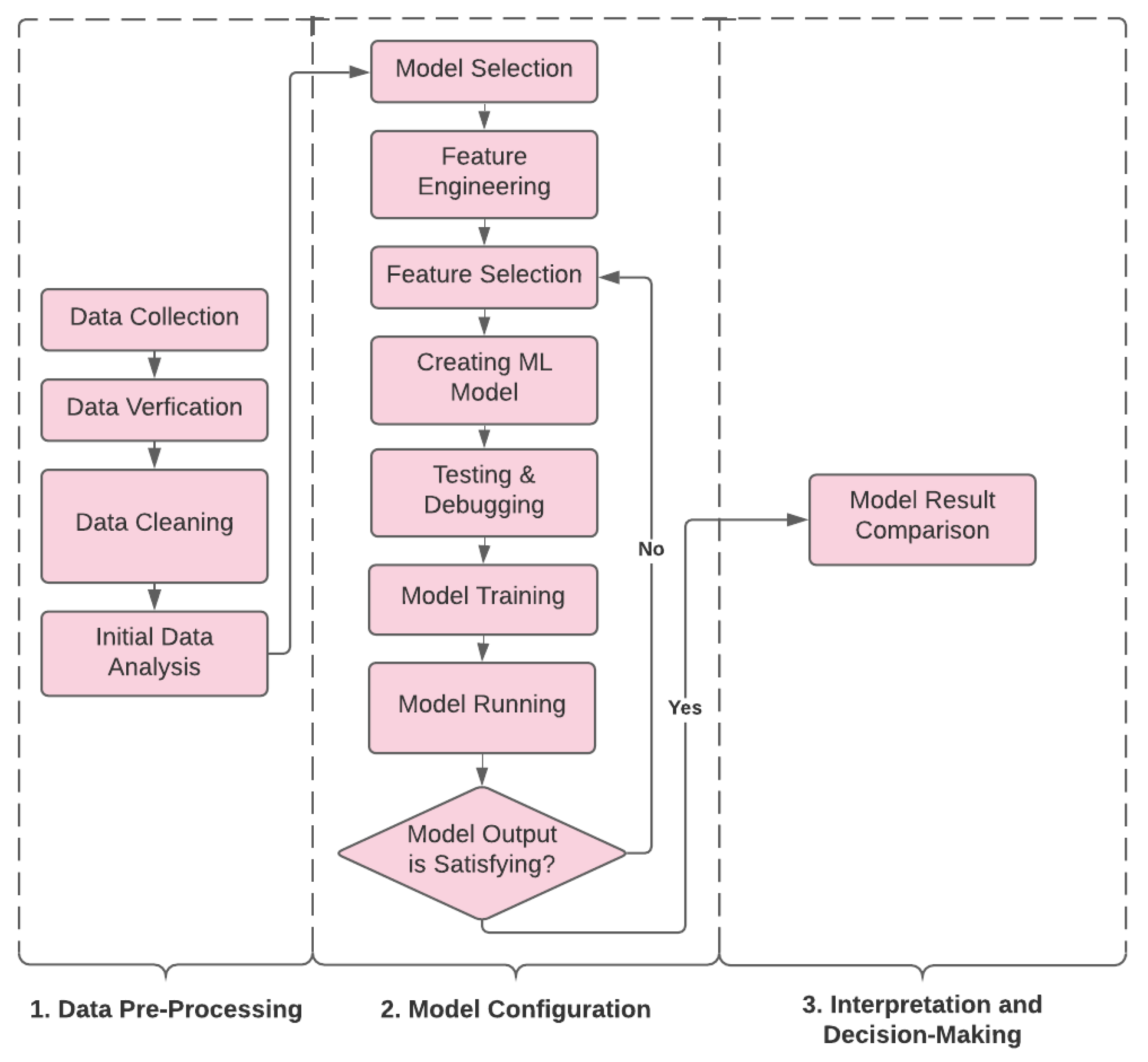
3.2. Data Pre-Processing

For the application of machine learning algorithms, data must be pre-processed in a mathematically feasible format. Therefore, data needs to be pre-processed to make it appropriate for the application of the modeling. Data pre-processing techniques included data reduction, data projection, and missing-data treatment. In data reduction, the size of the datasets decreases by means of feature selection. Data projection intends to transform all features into a conformed format and range. Missing-data treatments include deleting missing values and replacing them with the estimates if needed. Therefore, data needs to be pre-processed to make it appropriate for the application of the modeling.

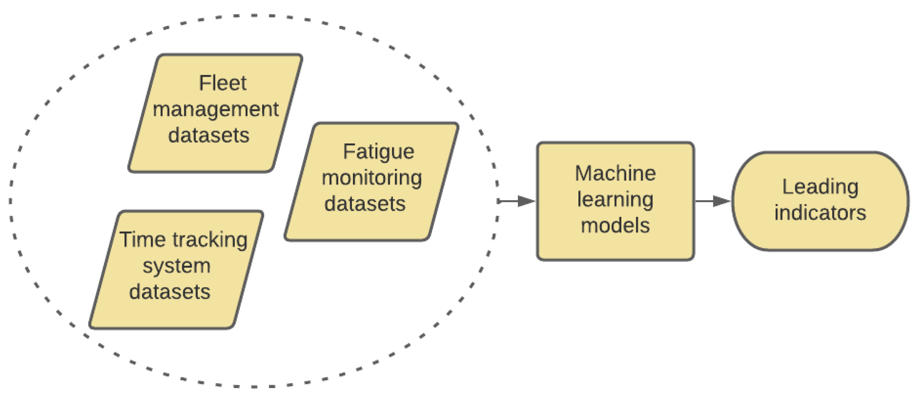
3.2.1. Data Integration

Each data set was linked to the fatigue monitoring data set based on a unique key. The FMS system separates equipment status and states. These tables also had to be integrated into a complex join. Data from FMS system, including status events of the equipment, were joined to the fatigue data by using a unique key. In order to have a categorized model, positive and negative samples are created from the fatigue monitoring data set, which are from the time operators were fatigued or not. After creating samples, other data from the attendance database such as overtime, worked hours and number of cycles from the Load-Dump cycles, were attached to them. In addition, the state of the haul truck at the time of the fatigue is integrated into the samples from the Load-Dump cycles data set. Finally, positive and negative samples are integrated together for the purpose of the model.

3.2.2. Data Cleaning

All of the datasets were cleaned, and missing data removed prior to input to the model. The process of cleaning data included correcting data types, removing incorrect, duplicate, incomplete, and corrupted data. The next step is handling missing values, like replacing them with anticipated data or dropping out the whole row from the data. In some cases, unwanted data has to be dropped from the data. In addition, the type of the data sets may need to be updated. Finally, multiple datasets should be merged.

In this study, missing data either was filled out with the estimated value, or the whole rows of them were dropped. Missing values can be handled by deleting the rows having null values. The rows which are having one or more column values as null can be dropped. In the case that we want to keep the row, Random Forest algorithm is used to fill out the missing values. It looks at the same data and predicts the missing value. Data are trained by the rows that have all values and predict values for the rows we have missing values. In order to join dump and load data, load IDs were created, which were comprised of shift index, shovel ID, Truck ID and arrive time. Some of these arrive times were missing; in which case an estimate was used based on the load-cycle data at the closest date and time. In the loads-dumps data set, almost 500,000 records were missing. Moreover, some of the data types and formats were changed for modeling purposes. Additionally, unwanted, duplicated, corrupted, and incorrect data were omitted from the data source.

3.2.3. Negative and Positive Samples

In this section, the process of how samples are created is explained. In this study, the categorical machine learning (ML) model is used. It means that data includes different data categories, which are positive and negative samples. The model predicts if the data is related to the positive sample, which means fatigue happened, or negative samples, which are related to the time without fatigue. Positive samples are derived from the fatigue monitoring data sets when a fatigue event is flagged by the system.

Negative samples were made from time frame when fatigue events did not happen. This sampling was done for each employee and equipment. In the process of data engineering, fatigue data is merged with status event data. Two factors are used for making negative samples. First, in order to find the number of samples, we looked at the ratio of the time frame that fatigue did not happen during a shift time for each employee. Second, we looked at each status event in a shift in a way that we have at least one sample for each status event. Therefore, these negative samples are created in an acceptable proportion ratio for the time frame that fatigue did not happen in a shift time and for each status event.

After these samples are created, other variables like time and attendance data, number of cycles, and overtime are merged with these samples. Moreover, other feature engineering is done for these samples. Finally, negative and positive samples are combined to have a big data set for the purpose of making the model. More details of what is done on the data in this process are explained in the feature engineering section.

3.2.4. Feature Engineering

Features are the numerical or categorical variables from the data sets that can determine the model prediction. They are independent, and ideally, there is little to no correlation between the features. Feature engineering has a vital role in data analysis and machine learning. Feature engineering meets a need for the generation and selection of useful features. It includes different steps of engineering as will be explained. Feature transformation, feature generation, and feature extraction are about making a feature from existing features [24]. Feature selection is about selecting a small set of features from the datasets to make it computationally feasible to use in a certain algorithm. Feature analysis and evaluation are the processes of evaluating the usefulness of the features, which is usually a part of feature selection [24].

In this study, all datasets are engineered in an appropriate way to be used in an XGBoost algorithm [25]. Fatigue data provided from the fatigue monitoring system were reviewed and divided into different categories. Among them, micro-sleeps and drowsiness were identified as the fatigue events of workers with low and critical fatigue levels. They were dependent variables of the model. All other available data like fleet management data, production cycles, and time and attendance were modeled as predictors and independent variables of the model. All features and variables used in different iterations of the modeling are shown in

Table 3. List of the variables based on the data source.

Data Source	Variables	Data Type and Example Data
Time and attendance	Employee ID	Integer (5 to 89,021)
	Common Equipment ID	Integer (205 to 841)
	Year	Integer (2014 to 2020)
	Month	Integer (1 to 12)
	Week	Integer (1 to 54)
	Day	Integer (1 to 31)
	Day of week	Integer (1 to 7)
	Day of year	Integer (1 to 366)
	Shift is end of month	Categorical Integer (0 and 1)
	Shift is start of month	Categorical Integer (0 and 1)
	Shift is end of quarter	Categorical Integer (0 and 1)
	Shift is start of quarter	Categorical Integer (0 and 1)
	Shift is end of year	Categorical Integer (0 and 1)
	Shift is start of year	Categorical Integer (0 and 1)
	Worked hour	Integer (0 to 13)
	Overtime	Integer (0 to 1)
	Overtime of previous shift	Integer (0 to 1)
Fleet management system (production and status)	Status—Delay Status—Down Status—Ready Status—Standby Number of cycles Number of cycles of previous shift Work Type Scheduled Work type Unscheduled Fleet_HTE—KOM960 Fleet_HTE—LEB282 Fleet_HTM—CAT793 Reason Description (Included of 70 different variables) State of Truck—Empty Driving State of Truck—Full Driving State of Truck—Loading State of Truck—None State of Truck—In Queue Waiting for Loading State of Truck—Spotting for Load Status Event Duration	Categorical Integer (0 and 1) Categorical Integer (0 and 1) Categorical Integer (0 and 1) Categorical Integer (0 and 1) Integer (1 to 121) Integer (1 to 121) Categorical Integer (0 and 1) Categorical Integer (0 and 1) Categorical Integer (0 and 1) Categorical Integer (0 and 1) Categorical Integer (0 and 1) Categorical Integer (0 and 1) Categorical Integer (0 and 1) Categorical Integer (0 and 1) Categorical Integer (0 and 1) Categorical Integer (0 and 1) Categorical Integer (0 and 1) Categorical Integer (0 and 1) Integer (2 to 167,932)
Fatigue monitoring system	Is Fatigue	Categorical Integer (0 to 1)

.

3.2.5. Features

This model was aggregated at the individual level (haul truck operators), with positive and negative samples as it is explained before. Since this model is a categorical model, a dependent variable is added to the data to show if a row of data is related to the fatigue event or not (True or False). Therefore, data are categorized into positive and negative samples. Positive samples are the rows of input data of the model that show actual fatigue events. Negative samples are the rows of data that are not fatigue events.

All the features were created for both positive and negative samples. Two different features were provided from the time and attendance data sets, overtime of current or previous shift and worked hours of the same shift for each sample. Moreover, some variables like day, week, month, and year were built from the attendance datasets. Loads and dumps data were part of the fleet management data represented by the load-dump cycle of the haul truck. They were used to create a feature of the number of cycles for the current shift and previous shift. Another feature that was provided from the cycle data is the states of the haul truck for each positive and negative sample. They were categorized into Queue Waiting for Load, Spotting for Load, Loading, Full Driving, Dumping, and Empty Driving. Status events datasets are used to find the status of the haul truck for the samples, such as Unscheduled work, Scheduled work, Ready, Delay, Down, Standby, and Event duration.

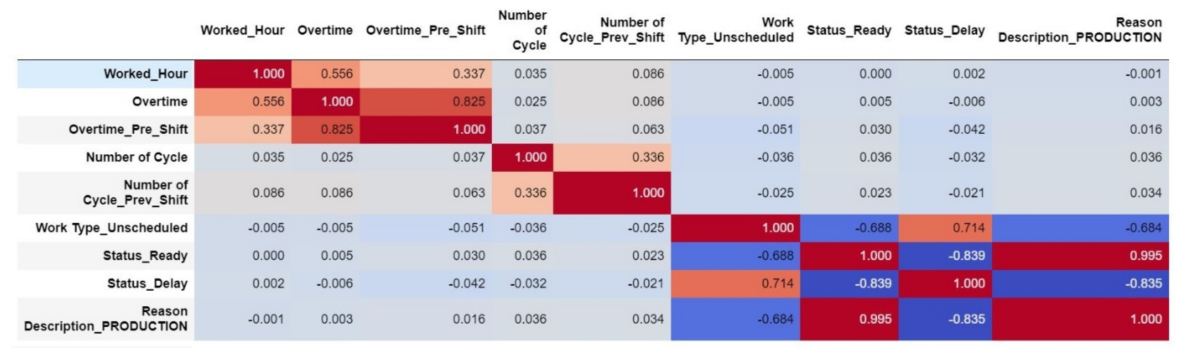
3.3. Data Visualization

Before creating any machine learning model and after data cleaning, it is necessary to do exploratory analysis. First, data should be examined before training the model. The Pandas library in Python was used to load data into a DataFrame structure for further manipulation. Then, some basic statistical analyses were generated, for example, the distribution of each countable variable (Figure 1). Other analyses produced linear correlations to observe the relationship between independent variables. Figure 2 displays the significant correlation of the variables.

As Figure 1 shows, 75% of the employees have 0.5 to 1.5 h of overtime, which can be seen from the worked hour data as well. On the other hand, the average number of cycles from the previous shift is almost 20 for most of the data. It also shows the right-skewed distribution, which identifies that most of the data have more than 50 cycles of the previous shift. Same data as overtime data from the worked hour graph shows that more than 75% of employees worked more than 12 h a shift. Other graphs display which day, month, and year have the higher rate of fatigue. The last graph shows which equipment ID has a higher rate of fatigue compared to others. Figure 2 demonstrates that some of the independent variables have a positive or negative correlation with more than R² = 0.7, which has darker red or blue color. Therefore, one of them is removed from the model to reduce the possibility of overfitting.

4. Methodology

Over the past several years, the UMODEL lab at University of Utah’s mining engineering department has been studying and modeling mine workforce fatigue. The approach has been examining fatigue through direct surveys of crews, developing tracking technology, and modeling fatigue using operational technology. This study investigates a model of the fatigue of individuals based on job demands and environmental factors. Therefore, it uses a machine learning (ML) algorithm applied to data from a surface mine to identify indicators of fatigue in operational datasets. The process and steps of this study are provided in Figure 3.

4.1. Modeling Approach

In general, there are three types of Machine Learning (ML) algorithms: supervised learning, unsupervised learning, and reinforcement learning. This study involves supervised learning, which includes a target variable (dependent variable) and a given set of predictors (independent variables or features) [25]. Dependent variables are predicted by the independent variables. An algorithm that maps inputs to desired outputs will be made with these independent variables. After the model is created, the training process continues until there is a satisfactory level of accuracy in the model [25]. Some of the examples of supervised learning consist of regression, decision tree, Random Forest (RF), K-Nearest Neighbour (KNN), logistic regression, etc. The algorithm used in this study is called eXtreme Gradient Boosting (XGBoost), which is an optimized distributed gradient boosting library [25]. It is designed to be highly efficient, flexible, and portable. It accomplishes machine learning algorithms under the Gradient Boosting framework. Gradient boosting gives a prediction model in the form of an ensemble of weak prediction models, which are typically decision trees. XGBoost algorithm provides a parallel tree boosting that can run them at the same time and solve many data science problems fast and accurately.

The fundamental idea of boosting is to integrate hundreds of simple trees with low accuracy to make a more accurate model. Every iteration will generate a new tree for the model. There are thousands of methods to generate a new tree. A common method is called the Gradient Boosting Machine [25]. It uses gradient descent to make the new tree based on previous trees. For this purpose, the objective function should be derived toward the minimum gradient direction.

XGBoost Algorithm

XGBoost model is a learning framework based on Boosting Tree models. XGBoost is based on gradient boosted decision trees designed for speed and performance. It has a strong expansion and flexibility and integrates multiple tree models to build a stronger ML model. Additionally, XGBoost uses a variety of methods to avoid overfitting [26].

In this study, the following parameters, known as hyperparameters, were adjusted to make the XGBoost model perform at its best:

• n_estimators: is the number of iterations in training. A very small n_estimators can result in underfitting, which diminishes the learning ability of the model. However, very large n_estimators will cause overfitting, which is not good either [26].
• min_child_weight: identifies the summation of sample weight of the smallest leaf nodes to prevent overfitting.
• max_depth: is the maximum depth of the tree. The bigger depth of the tree makes the tree model more complex and the fitting ability stronger. However, the model is more likely to overfit.
• subsample: is the sampling rate of all training samples.
• colsample_bytree: is the feature sampling rate when constructing each tree. In this task, this is equivalent to the sampling rate of the landmark gene.
• learning_rate: is a tuning parameter in an algorithm that defines the weight at each step while moving toward a minimum of a loss function. It is a very important parameter that needs to be adjusted in every algorithm. It greatly affects the model performance. To make the model more robust, we can decrease the weight of each step.

4.2. Model

For this study, different iterations of the model were conducted using available data subsets as dependent variables. The machine learning procedure diagram is displayed in Figure 4. All of the features (independent variables) were created from the available data sets for each individual. The dependent variable predicts true fatigue events from non-fatigue events. True fatigue events are classified as positive and non-fatigue events are considered negative. All independent variables in these models, also known as features, are representations of some of the mine’s operation data sets. These features contain values such as the status of the haul truck in the operation cycle, over time, and the working hours of the operator (see Table 3).

Data were divided into two sets: 80% constituted the training data set, and 20% constituted the validation data set. The purpose of these models was to determine the features that can predict fatigue to maximize model scores. In these models, only data subsets with micro-sleeps were modeled. From 209,710 possible events, only 1073 contained micro-sleep with critical and low fatigue reviews in the data sets to train and validate the XGBoost algorithm. After initial data exploratory analysis, this study refined models to predict operator fatigue. Then, possible iterations to choose the best features were conducted to predict fatigue and the possibility of including all available feature sets that drive fatigue. Data for these models were constrained to the number of days contained in the fatigue data. Thus, the models were created using data from 7 November 2014 to 23 June 2020.

After engineering data, data should be numeric for applying the selected algorithm. Therefore, every feature is checked, and its format is changed to be numeric. All of the categorical features are used to make several features with 0 and 1 values as they can be appropriate for this model. The status events and production datasets create over fifty numerical variables, including status, reason description, work type, and the state of the haul truck in the time of fatigue.

In order to get the best possible results out of the selected algorithm and leverage the maximum power of the algorithm, hyperparameters should be tuned. This selected algorithm provides an extensive range of hyperparameters. XGBoost is a powerful machine learning (ML) algorithm that has shown strong performance at picking up patterns in the data by automatically tuning thousands of learnable parameters. In tree-based models, like XGBoost, the learnable parameters are the choice of decision variables at each node, creating more design decisions and, as a result, a wider range of hyperparameters. These parameters were specified by hand to the algorithm and fixed throughout a training phase. As mentioned earlier, for this model, there are hyperparameters including maximum depth of the tree, number of trees to grow, number of variables to consider when building each tree, minimum number of samples on a leaf and fraction of observations used to build a tree. These are some of the model parameters used in this study: learning rate: 0.05, maximum depth of tree: 5, number of trees: 100, minimum child weight: 500, fraction of observations used to build a tree (subsample): 1.

4.2.1. Model Iterations

For the first iteration of the modeling, all the available features were used to model fatigue. Variables for the second, third and fourth iterations of modeling are determined by results from the first iteration. Two top features from the first model iteration are the number of cycles and overtime of the employees. In order to see the effect of other features, they are removed for the second iteration of the modeling. Another top feature of the first model was employee ID. It shows that some individuals have a higher rate of fatigue compared to others. Therefore, two different models were created based on the employee ID: employees with higher rates of fatigue and employees with lower rates of fatigue. Results from both models demonstrate that different indicators affect fatigue of these two groups.

4.2.2. Model Evaluation

After data training and model debugging, each model result was interpreted, and if the result is accepted, the model is evaluated. Different approaches are available for evaluating the model. One way of the model evaluation is the model score or R². This score is usually from the validation data set. The higher the model score, the better the model performs. Next for each tree-based algorithm is Gini index. The Gini index calculates the degree of probability of a specific variable that is wrongly being classified when chosen randomly for each tree, which works on categorical variables. The degree of Gini index varies from 0 to 1:

• Where 0 describes that all the elements be allied to a certain class.
• The Gini index of value as 1 denotes that all the elements are randomly distributed across various classes.
• A value of 0.5 shows the elements are uniformly distributed into some classes.

The next method of model evaluation, which is used here, is the confusion matrix. Since this model used classification predictions, there are four types of outcomes that could occur, which are often plotted on a confusion matrix as an outcome of the model.

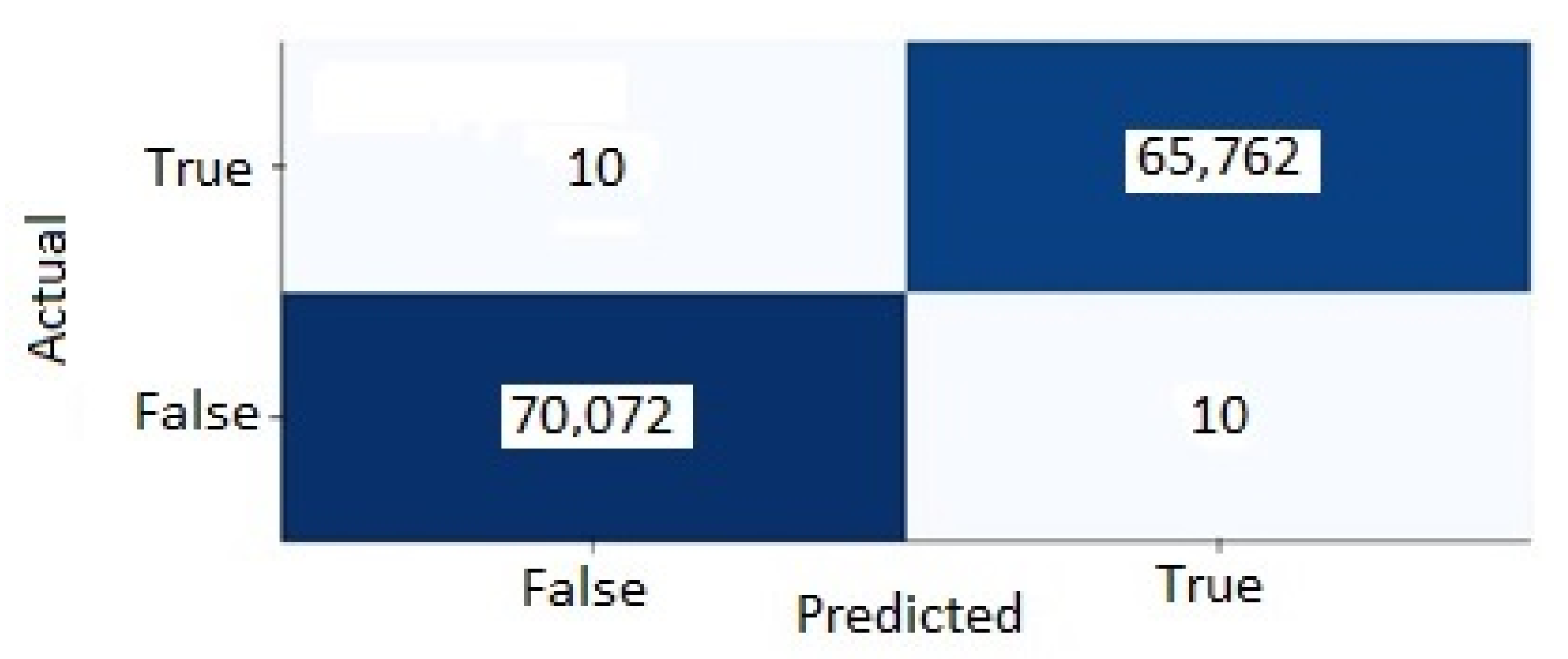
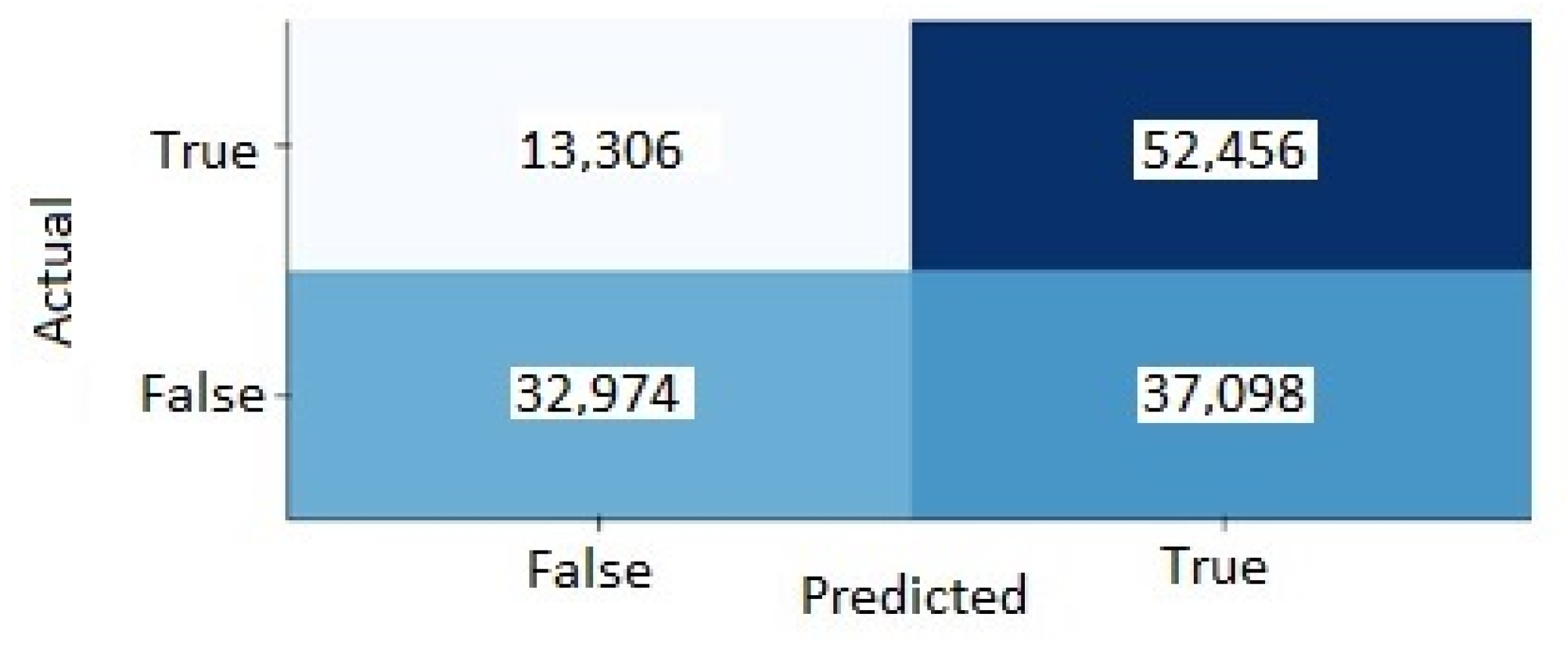
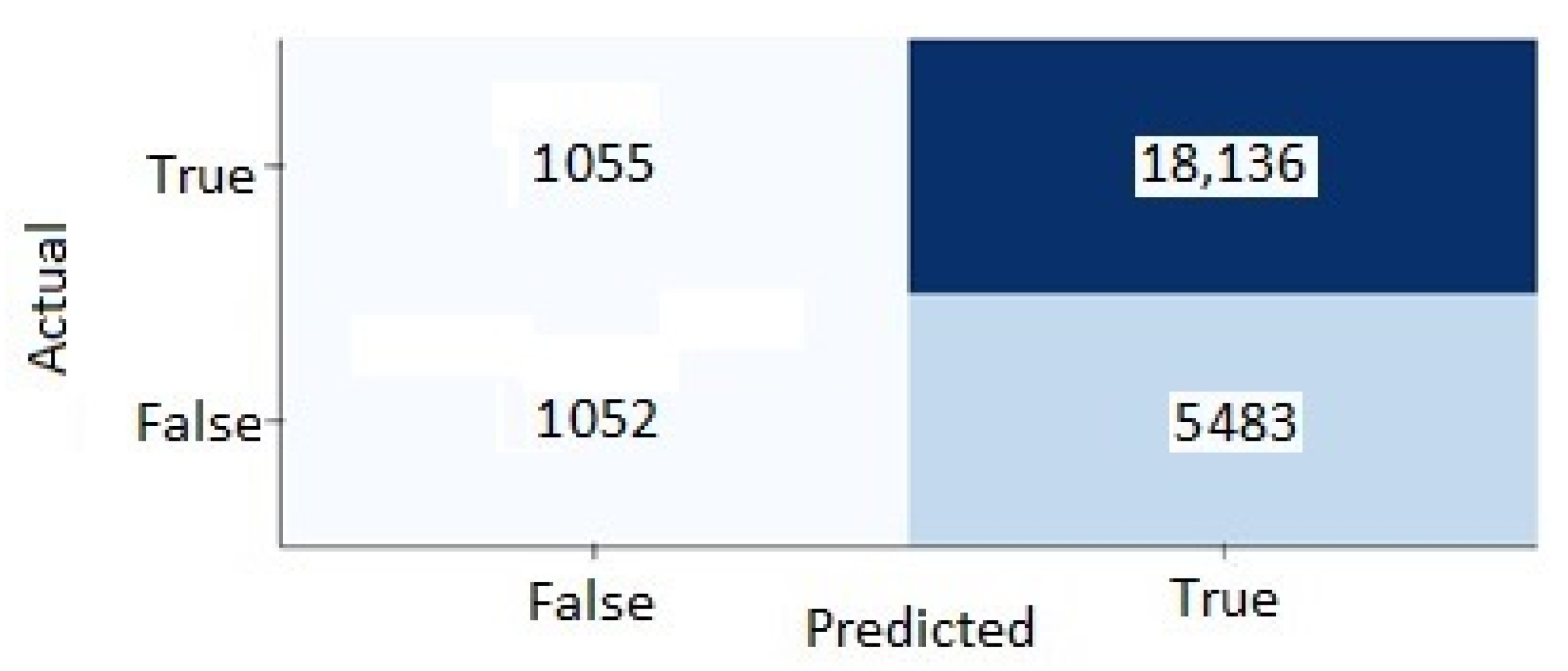
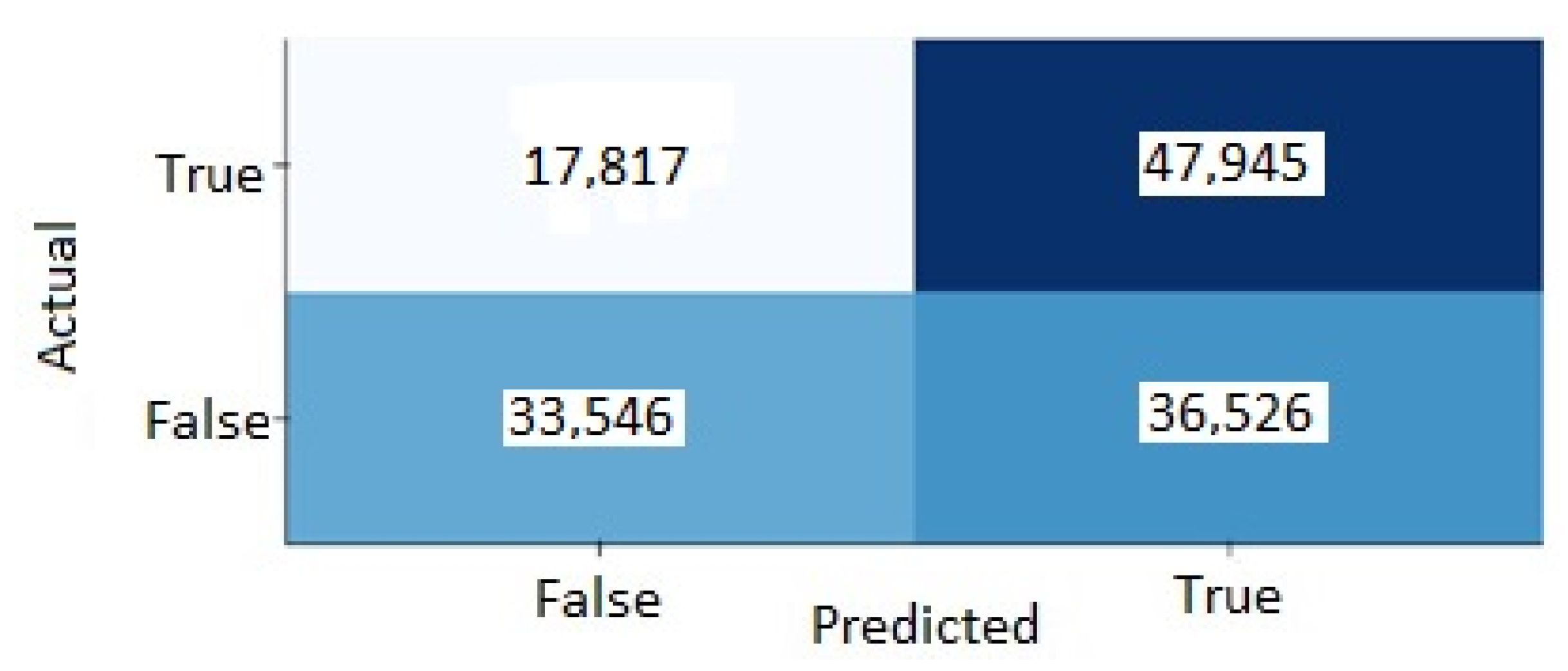
• True positives: when the model predicts a fatigue event which is an actual fatigue event in the data sets.
• True negatives: when the model predicts that an event is not fatigue and it is not an actual fatigue event in the data sets.
• False positives: when the model predicts a fatigue event that is not an actual fatigue event in the data sets.
• False negatives: when the model predicts that an event is not fatigue and it is an actual fatigue event in the data sets.

5. Results

5.1. Model Results

Different iterations of the model were created, and five of them were selected as they performed better. All of these model iterations work well as their scores are acceptable. The first model with all of the features works great. It shows that employee ID, event duration, worked hour, number of cycles from the previous shift, shift index, day, day of year, day of week, and overtime of the previous shift have the biggest effect on the fatigue of the haul truck operators. It shows that some individuals have a higher rate of fatigue compared to others, as the top feature of the model shows. Crews seem to have outliers that are the main drivers of fatigue events [6]. Another parameter from this model is overtime from the previous shift, which denotes more fatigue happened for employees who have more overtime from the previous shift. Moreover, it demonstrates that the state of the haul truck categorized to such as empty-driving and full-driving can drive fatigue of the operator. All the top features are displayed in

Table 4. Model performance results.

Model	Independent Variables	Score	Top Features
First model	Employee ID Common Equipment ID Year Month Week Day Day of week Day of year Shift is end of month Shift is start of month Shift is end of quarter Shift is start of quarter Shift is end of year Shift is start of year Worked hour Overtime of previous shift Status—Down Status—Standby Number of cycles of previous shift Work Type Scheduled Work type Unscheduled Fleet_HTE—KOM960 Fleet_HTE—LEB282 Fleet_HTM—CAT793 Reason Description (Included of 70 different variables) State of Truck—Empty Driving State of Truck—Full Driving State of Truck—Loading State of Truck—None State of Truck—In Queue Waiting for Loading State of Truck—Spotting for Load Status Event Duration	0.98	Employee ID Event Duration Worked Hour Number of Cycle Previous Shift Shift Index Day Day of year Day of week Overtime Previous Shift Common Equipment ID Is Quarter End Shovel Machine Month Week State Truck Full Driving State Truck Empty Driving
Second model	Employee ID Common Equipment ID Year Month Week Day Day of week Day of year Shift is end of month Shift is start of month Shift is end of quarter Shift is start of quarter Shift is end of year Shift is start of year Worked hour Overtime Status—Down Status—Standby Number of cycles Work Type Scheduled Work type Unscheduled Fleet_HTE—KOM960 Fleet_HTE—LEB282 Fleet_HTM—CAT793 Reason Description (Included of 70 different variables) State of Truck—Empty Driving State of Truck—Full Driving State of Truck—Loading State of Truck—None State of Truck—In Queue Waiting for Loading State of Truck—Spotting for Load Status Event Duration	0.83	Employee ID Shift Index Event Duration Number of Cycle Common Equipment ID Worked Hour Day of Year Week Work Type Unscheduled Shovel Machine Work Type Scheduled Day of Week Day State Truck Full Driving State Truck Empty Driving Fleet HTE—KOM960 State Truck Queue Waiting for Load Fleet HTE—CAT793 Fleet HTE—LEB282 Year
Third model	Employee ID Common Equipment ID Year Month Week Day Day of week Day of year Shift is end of month Shift is start of month Shift is end of quarter Shift is start of quarter Shift is end of year Shift is start of year Worked hour Status—Down Status—Standby Work Type Scheduled Work type Unscheduled Fleet_HTE—KOM960 Fleet_HTE—LEB282 Fleet_HTM—CAT793 Reason Description (Included of 70 different variables) State of Truck—Empty Driving State of Truck—Full Driving State of Truck—Loading State of Truck—None State of Truck—In Queue Waiting for Loading State of Truck—Spotting for Load Status Event Duration	0.82	Employee ID Shift Index Event Duration Worked Hour Common Equipment ID Day of Year Week Shovel Machine Day Day of Week Work Type Unscheduled Work Type Scheduled State Truck Full Driving Fleet HTE—KOM960 State Truck Empty Driving State Truck Queue Waiting for Load Year Fleet HTE—LEB282 Fleet HTE—CAT793 Month
Fourth model (With employees with a higher rate of fatigue)	Common Equipment ID Year Month Week Day Day of week Day of year Shift is end of month Shift is start of month Shift is end of quarter Shift is start of quarter Shift is end of year Shift is start of year Worked hour Status—Down Status—Standby Work Type Scheduled Work type Unscheduled Fleet_HTE—KOM960 Fleet_HTE—LEB282 Fleet_HTM—CAT793 Reason Description (Included of 70 different variables) State of Truck—Empty Driving State of Truck—Full Driving State of Truck—Loading State of Truck—None State of Truck—In Queue Waiting for Loading State of Truck—Spotting for Load Status Event Duration	0.83	Shift Index Common Equipment ID Event Duration Day Worked Hour Day of year Shovel Machine Day of Week State Truck Full Driving Week State Truck Empty Driving Year Month State Truck Queue Waiting for Load Fleet HTE—KOM960 Work Type Unscheduled Is Month End
Fifth model (With employees with a lower rate of fatigue)	Common Equipment ID Year Month Week Day Day of week Day of year Shift is end of month Shift is start of month Shift is end of quarter Shift is start of quarter Shift is end of year Shift is start of year Worked hour Status—Down Status—Standby Work Type Scheduled Work type Unscheduled Fleet_HTE—KOM960 Fleet_HTE—LEB282 Fleet_HTM—CAT793 Reason Description (Included of 70 different variables) State of Truck—Empty Driving State of Truck—Full Driving State of Truck—Loading State of Truck—None State of Truck—In Queue Waiting for Loading State of Truck—Spotting for Load Status Event Duration	0.82	Shift Index Event Duration Shovel Machine Day of year Worked Hour Common Equipment ID Day Day of Week Work Type Unscheduled Week Work Type Scheduled State Truck Full Driving State Truck Empty Driving Fleet HTE—KOM960 Fleet HTE—LEB282 State Truck Loading State Truck Queue Waiting for Load Month Fleet HTE—CAT793 Is Month End

.

For the second iteration of the model, the number of cycles and overtime of the employee from the previous shift substitutes with the number of cycles and overtime of the same shift. The same result as the previous model shows that employee ID has the highest effect on fatigue. Some of the other top features of this model are shift index, event duration, number of cycles, common equipment ID, worked hour, day of year, week, work type unscheduled, and shovel machine.

After analyzing two first model outcomes, to see the effect of the top features on the model prediction, some of them are removed from the data set to run the third step of the modeling. Hence, the third model was created with all features except the number of cycles and overtime of the previous shift and the same shift. The top feature of the third model is employee ID, which shows the same information as the two first models. Other topmost features are shift index, event duration, worked hours, and equipment ID. It shows that some specific fleets have a higher rate of fatigue compared to others. Overall, it shows other important features from the model like day, week, work type, and state of the haul truck are more effective on fatigue.

A top feature of the first three models is employee ID. Therefore, to see the effect of employee ID on the model prediction, we decided to create the fourth and fifth steps of the modeling for two groups of employees with a higher and lower rate of fatigue. The fourth model also performs well for employees with a higher rate of fatigue. It shows that top features are included in the status shift index, followed by the equipment ID, event duration, day, worked hour, day of year, shovel machine, day of week. It also demonstrates that the state of haul truck of full driving has a higher effect compared to empty driving.

Another iteration of the model was conducted for the employees with a lower rate of fatigue. Model outcome shows that shift index event duration, shovel machine, day of year, and worked hours, followed by equipment ID, day, day of week, work type unscheduled, and week have effects on the fatigue. Other top features of this model are the state of haul trucks and also shows that some fleets have higher fatigue compared to others. In Table 4, the results of the best-performed model are displayed. Later, a comparison of the model iterations is presented.

All the model outputs illustrate that the state of the haul truck can increase the fatigue of the operators. Among all the different states of the haul truck, empty driving has a greater impact, which is not surprising since the truck needs to be moving for the system to work. Another observation from the models is that, after empty driving, full driving also has an effect on the fatigue of the operators. It may be because of the monotonous task while driving to the destination of dumping of loading. It also may be due to long-distance driving.

5.2. Gini Index

The Gini index or Gini coefficient computes the degree of probability of a specific variable that is wrongly being classified when chosen randomly. The Gini index estimates the amount of probability of a specific feature that is incorrectly classified when selected randomly in the decision tree. If all the elements are linked with a single class, then it can be called pure. The Gini index varies between values 0 and 1, where 0 identifies the purity of classification, and all the elements belong to a specified class or only one class exists there, and 1 expresses the random distribution of elements across different classes. Additionally, the value of 0.5 shows an equal distribution of elements over some classes. In every decision tree algorithm, Gini index can help to find the best-chosen samples for the best-performed tree. The best-chosen samples for the decision tree for each iteration of the models are shown in

Table 5. Gini index of the models.

Model	Gini Index
First model	0
Second model	0.46
Third model	0.48
Fourth model	0.37
Fifth model	0.47

. Gini index is the evaluation method during the process of the model training; however, a confusion matrix is calculated after the model is made.

5.3. Confusion Matrix

Confusion matrices demonstrate counts from predicted and actual values. It shows the score of the model and how accurate the model predicted testing data. In the confusion matrix, there are four different values. The output TN means True Negative, which shows the number of negative samples classified by the model accurately. Likewise, TP stands for True Positive, indicating the number of positive samples predicted by the model accurately. FP shows False Positive values, the number of actual negative examples classified by the model as positive. FN stands for False Negatives value, which is the number of actual positive samples classified by the model as negative. Figure 5, Figure 6, Figure 7, Figure 8 and Figure 9 represent the confusion matrices of all four model iterations. One of the commonly used metrics for classification models is accuracy. The accuracy of the model can be calculated by summation of accurate prediction over a summation of all classified samples in the confusion matrix, as Equation (1) shows.

Table 6. Model accuracy.

Model	Accuracy
First model	0.99
Second model	0.63
Third model	0.60
Fourth model	0.74
Fifth model	0.60

represents the accuracy of the models.

$$(\frac{TN+TP}{TN+TP+FP+FN}),$$

(1)

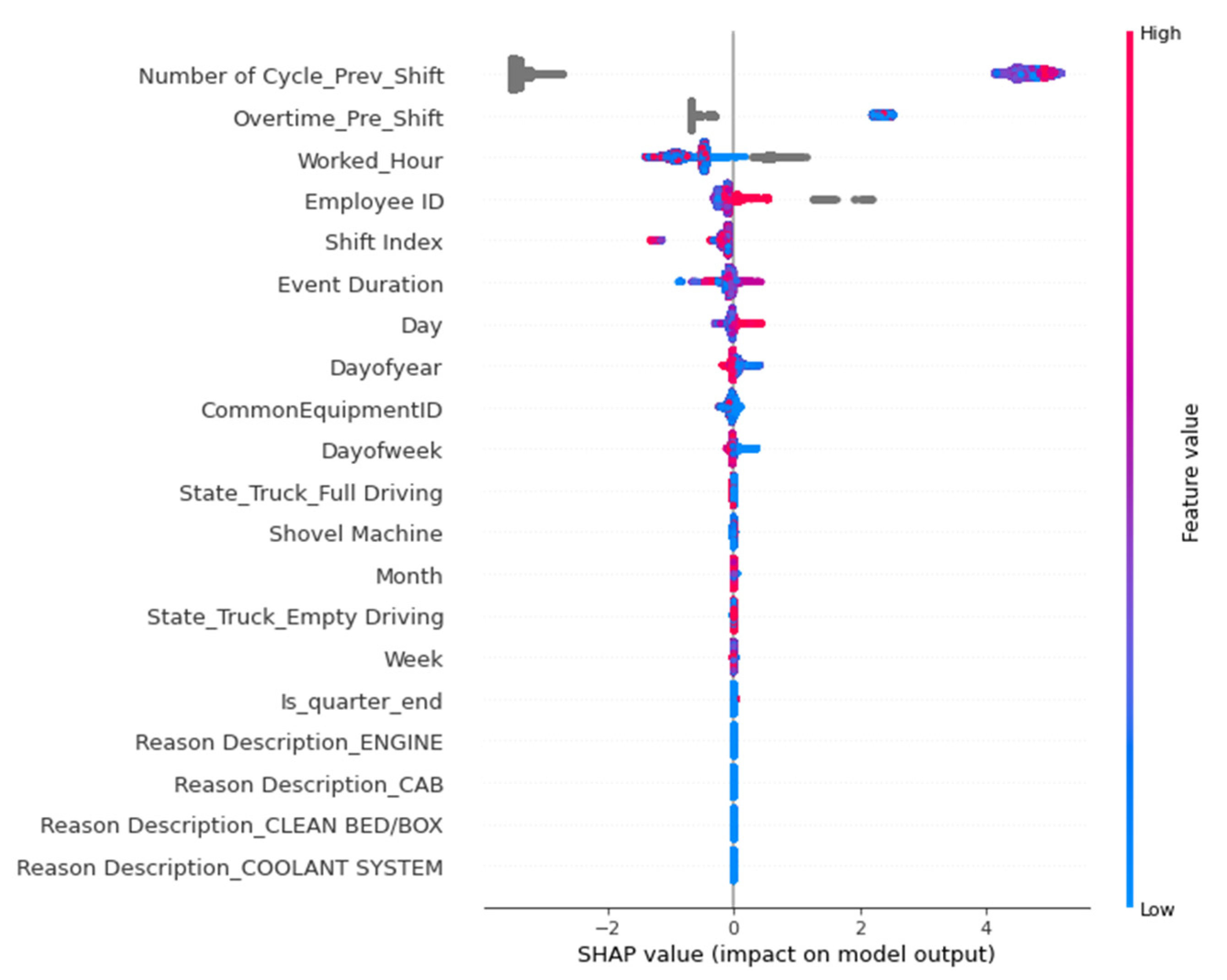
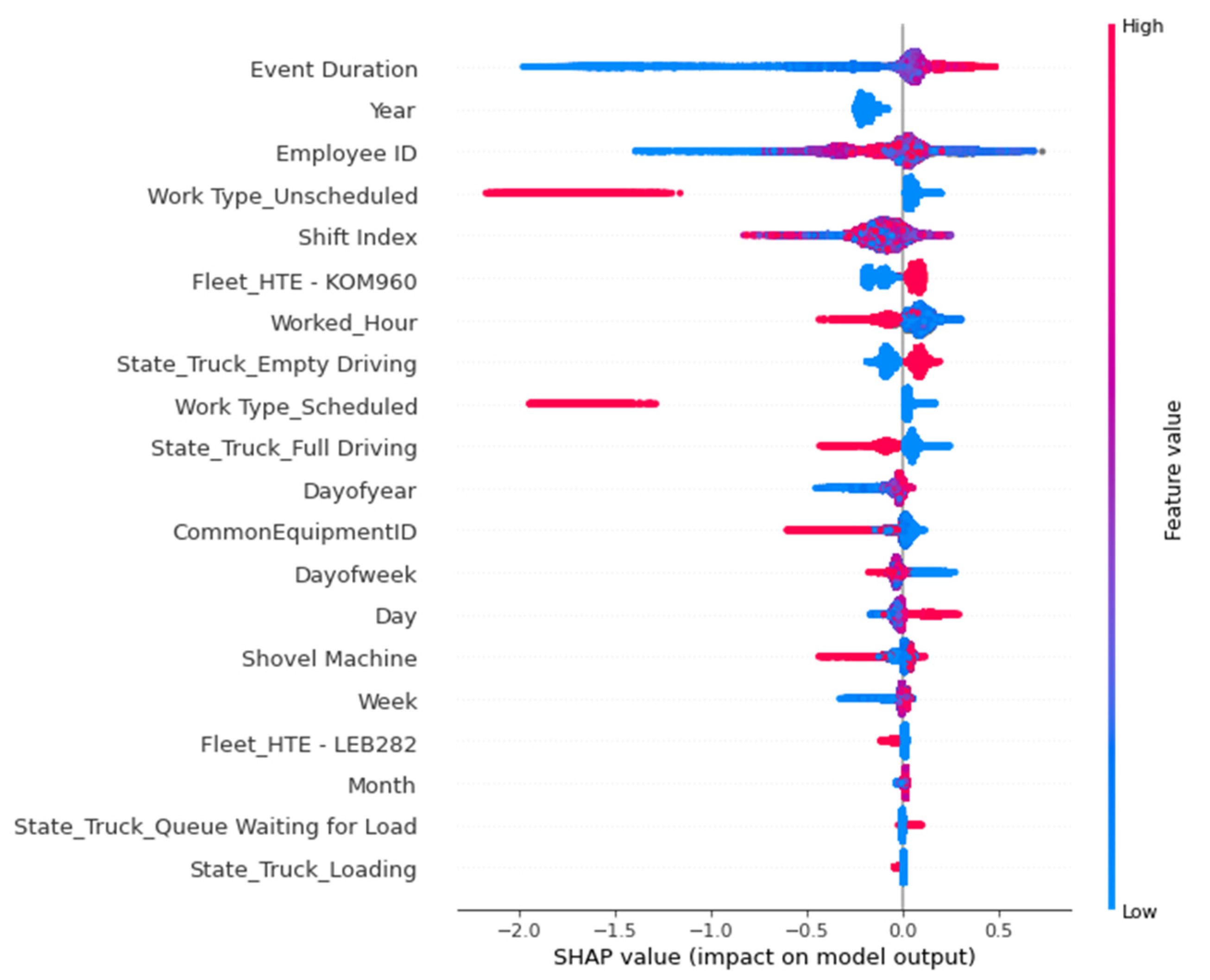
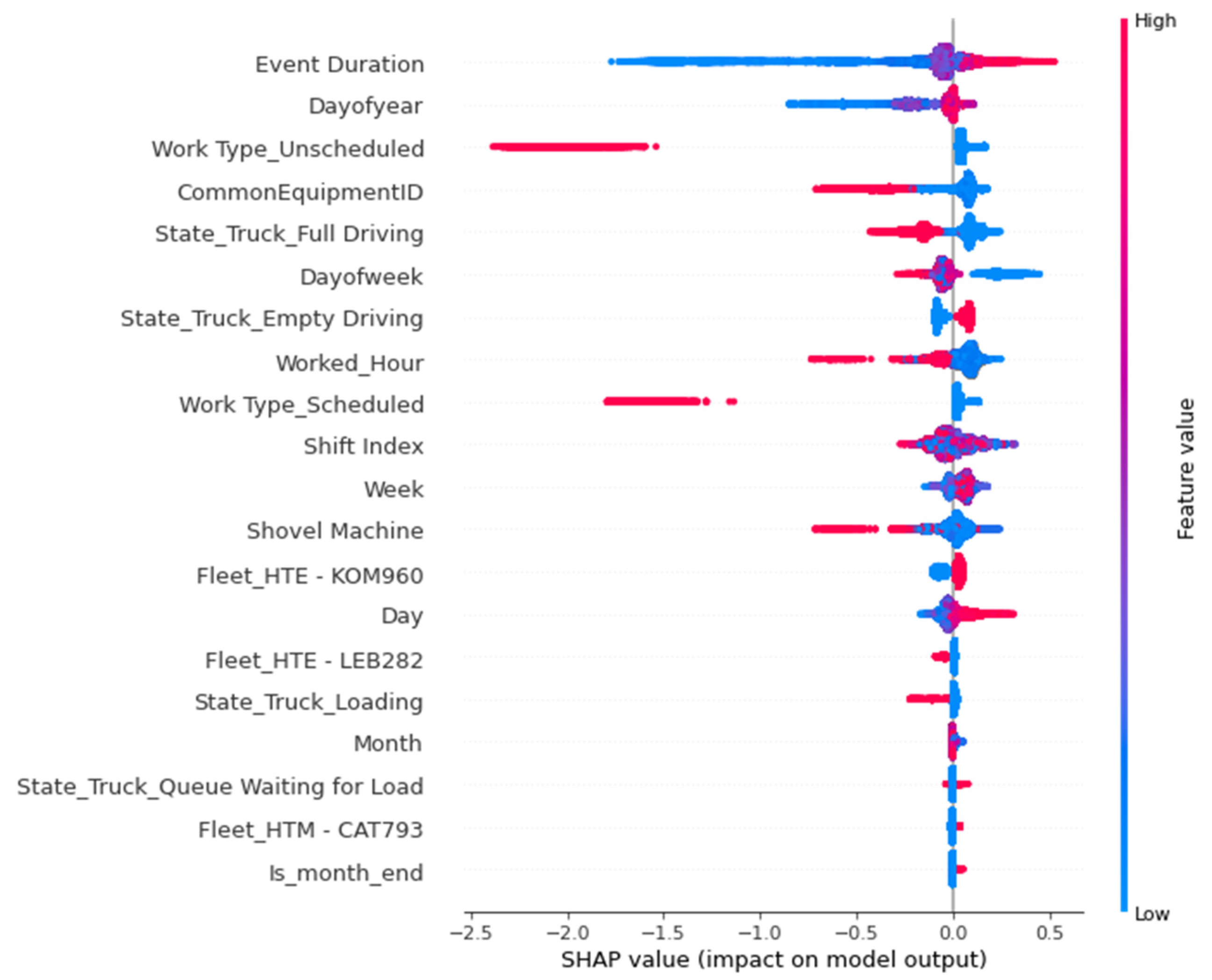
5.4. SHAP Values of the Models

SHAP values are based on Shapley values, a concept coming from game theory. This game theory requires a game and some players. Here, in the machine learning model, the game reproduces the outcome of the model, and the players are the features included in the model. Shapley quantifies the contribution of each player to the game, and the contribution of each feature brings to the prediction of the model. In fact, SHAP is about the local interpretability of a predictive model. Therefore, SHAP values of the five different iterations of the models are provided in Figure 10, Figure 11, Figure 12, Figure 13 and Figure 14.

They show the feature value on the model and the SHAP value of each value of the features. Red presents the higher value of the feature, and blue presents the lower value of the feature. For instance, the employee ID with the higher value positively impacts the model output. Adversely, unscheduled work type negatively impacts the fatigue model output, which means that a higher value of the unscheduled work type increases the fatigue of the operator. Another interesting finding from the SHAP value plot is that in the case of driving with a full haul truck, a higher value has a negative effect on the fatigue model output. Therefore, these plots can be utilized to interpret the result of the model in detail and in a more nuanced way.

5.5. Model Iterations Comparison

As discussed previously, several different model iterations were created to explore which features have the higher effects on fatigue. Five different iterations are provided for comparison. Details of them are provided in

Table 7. Comparison of the models.

Model	Top Feature	Score	Percentage of Samples That Predicted Correctly
First model	Employee ID	0.99	100%
Second model	Employee ID	0.83	63%
Third model	Employee ID	0.82	60%
Fourth model	Shift Index	0.83	74%
Fifth model	Shift Index	0.82	60%

for comparison. For the first iteration, all of the available engineered features such as the number of cycles and overtime of the previous shift are used. This model has a score of 0.98. Figure 4 displays the confusion matrix of the models, which shows that the model works decently. As it illustrates, only 20 samples are not predicted correctly. It shows that employee ID has the highest effect on fatigue. Employee ID illustrates that each individual has a different rate of fatigue events. Moreover, it shows employee ID, event duration, worked hours, and shift index has effects on the fatigue of the individuals. It also shows that the number of cycles of the previous shift has an effect on fatigue. For the second iteration, the same features are used, except the number of cycles and overtime from the previous shift are dropped from the model, and instead, those features from the same shift are used. However, the score of the model is lower, and it demonstrates the same top features as the first model, with employee ID having the highest effect on the model.

For the third model iteration, employee ID and for the fourth and fifth models, shift index is a top feature. The second, third, fourth, and fifth models are not performing well as the first model, but they demonstrate other important features of the model. For example, event duration, shovel machine, equipment ID, and day are the features that model outcome shows as top features. The confusion matrix for these models shows that the model has some errors in predicting fatigue in these models. The second model has a significant error in predicting samples, 13,306 and 37,098, respectively true and false samples are predicted wrong by the model. The third model could not predict 17,817 true samples and 36,526 false samples correctly. The fourth model also predicted 1055 and 5483 true and false samples wrong. In the last model, 26,657 and 17,242 true and false samples are predicted wrong. As the confusion matrix represents, fatigue is predicted by the second, third, and fourth models mostly when a sample is a fatigue event, which means they are positive samples. However, the fifth model predicts better when the sample is not a fatigue event, which means that samples are negative samples.

6. Discussion

The model output identifies the variables that have the greatest impact on all fatigue events.

Table 8. Top features by data classification.

Data Category	Feature Rank	Feature
Time and attendance	1	Employee ID
	3	Worked Hour
	5	Shift index
	6	Day
	7	Day of year
	8	Day of Week
	9	Overtime Previous Shift
	11	Is quarter end
	13	Month
	14	Week
Fleet management system (production and status)	2	Event Duration
	4	Number of Cycle Previous Shift
	10	Common Equipment ID
	12	Shovel Machine
	15	State Truck Full Driving
	16	State Truck Empty Driving

illustrates the most important features and their data sources from the best-performed model (first model). The model results admit current understanding of fatigue, at the same time providing some interesting new insights into work and environmental factors that potentially cause fatigue for individuals. Fatigue events are clustered consistently within a group of individuals. Since the model outcome represents employee ID as one of the top factors, we can conclude that individual factors greatly affect fatigue. Based on the study by Drews F. (2020), this can be because of different factors like individual sleep efficiency, clinical conditions, life and event stressors, and personality factors [18]. From the model outcome and as it is expected, each individual has a different rate of fatigue.

Drews F. (2020) conceptual fatigue model examines previous shift factors that have effects on the sleep history and, finally, fatigue of the individual [18]. It also represents work demand as a big factor of fatigue, which has physiological and psychological impacts on the individual. A similar result from this study outcome shows that overtime work and the number of cycles of the previous shift highly impact fatigue. The number of cycles and overtime show the burden of the work demand for the operators. Similarly, the state of the haul truck driver is another factor that drives fatigue. They demonstrated the state of the haul truck in the load-dump cycle when fatigue happened. Another finding from these models shows that the shift index is a factor that drives fatigue, which shows fatigue rate is higher in some specific shifts. Additionally, the outcome from the models shows that full-driving and empty-driving have a higher fatigue rate than other states, which full-driving affects fatigue more compared to empty-driving. It can be because of the monotonous task for a long time compared to when they dumped, loaded, or waited in a queue. Moreover, model results offer that some specific work types, like unscheduled ones, increase the rate of fatigue. It implies that any unscheduled tasks like delays in the cycles make the operator more vulnerable to fatigue due to waiting time. It also shows that cycles after that will have a higher risk of fatigue. Other variables from the model are shovel machine, equipment ID, day, week, month, and is the end of the month, which suggest a pattern in the fatigue time for individuals. As the model shows, the higher duration of the fatigue event, the more fatigue event happens for the operator, which shows a more serious issue.

Results from the model with higher rates of fatigue and lower rates of fatigue demonstrate that different indicators affect the fatigue of these two groups. In addition, they display that some fleets have a higher rate of fatigue compared to other fleets. These models also show that unscheduled work type has a higher impact on the fatigue of the employees with a higher rate of fatigue.

These outcomes can help the health and safety managers understand the magnitude of the mine site’s fatigue issues. Looking at the significant effect of the individual factors on fatigue and work environment factors propose more attention to individuals by the health and safety managers. The model can be used to justify targeted fatigue training for each individual that has a higher fatigue risk to take care of their individual factors like sleep quantity and quality. Another approach would be providing insight to managers and supervisors to target more flexible interventions (shift schedule, breaks, etc.) for individuals with a higher rate of fatigue or a greater fatigue duration. Supervisors can have more targeted engagement with operators during monotonous tasks like empty haul state. The number of cycles shows if they worked the whole shift or had some equipment downtime. The high number of cycles shows high work-demand during the shift. Similarly, overtime shows the burden of the work, which even asks for work after the shift ends. From the health and safety perspective, they can manage to support and check individuals with a lower rate of break. Another issue is the delay in production, which supervisors can manage by being alert to check these operators more often.

These model outcomes proved that factors that drive fatigue for each individual are different, and the mining industry needs to have individualized flexibility of health and safety programs versus a common general program or a tool to detect fatigue. Current fatigue monitoring systems are not able to consider these individual differences in a comprehensive way. A more comprehensive fatigue monitoring and prediction program can likely prevent the consequences earlier than lagging systems. Looking at the individual’s condition is very important and helpful in improving health and safety situations. Moreover, work demand is another factor that health and safety programs could look at to control fatigue. Such as having specific controls and supervision in a time of higher work demand.

7. Conclusions

Although this study tries to show the application of machine learning algorithms in health and safety management mining operations, its finding helps to understand the individual’s fatigue. This finding, along with a previous study from the authors, confirms that fatigue is caused by a wide variety of individual and work environmental factors. Some of them are easy to quantify, and some are difficult. Since fatigue is the complex interaction between human behavior and the dynamic work mines environment, it is tough to make a comprehensive model that shows all of the variables driving the fatigue of each individual. Previous models examined the issues at an aggregated level using operational data sets; this study clearly shows individualized factors from the operational data sets that have effects on the individual’s fatigue.

As it is mentioned before, JDR model is related to risk factors associated with job stress, such as job demands and job resources [8]. Our model uses these job demands factors that could contribute to physical or physiological stressors for the operators like the number of cycles, overtime, worked hours, and other production variables, etc. However, this model is limited by the available variables from the data sets, it would be helpful to add other job-related factors for the next study, like off days and any break time for the operators. In addition, other personal factors like sleep duration, efficiency, exercise, food and drink consumption would also aid in developing a more comprehensive understanding of fatigue risk for individuals.

All developed models have a high score greater than 0.8, but the first iteration has the highest score by far. However, this model is used for guiding other iterations of the additional models. These subsequent models did not achieve as high a score as the initial model. Findings of the first model show that fatigue is clustered around certain Individual’s and factors from the previous shift are very important. The important point is how to find these factors from the available data. It is recommended for the next research to use individual factors like fitness, sleep history, commute hours, diet, and other individual factors to explore more possible indicators of fatigue. Another recommendation is to use the Neural Network model to understand the combination of the parameters that have effects on the individual’s fatigue.

References

1. Sadeghniiat-Haghighi, K.; Yazdi, Z. Fatigue management in the workplace. Ind. Psychiatry J. 2015, 24, 12. [Google Scholar] [PubMed]
2. Halvani, G.H.; Zare, M.; Mirmohammadi, S.J. The relation between shift work, sleepiness, fatigue and accidents in Iranian Industrial Mining Group workers. Ind. Health 2009, 47, 134–138. [Google Scholar] [CrossRef] [PubMed]
3. Bauerle, T.; Dugdale, Z.; Poplin, G. Mineworker fatigue: A review of what we know and future directions. Min. Eng. 2018, 70, 33. [Google Scholar] [PubMed]
4. Qing, W.; BingXi, S.; Bin, X.; Junjie, Z. A perclos-based driver fatigue recognition application for smart vehicle space. In Proceeding of the 2010 Third International Symposium on Information Processing, Qingdao, China, 15–17 October 2010. [Google Scholar]
5. Wang, L.F.; Liu, J.Q.; Yang, B.; Yang, C.S. PDMS-based low cost flexible dry electrode for long-term EEG measurement. IEEE Sens. J. 2012, 12, 2898–2904. [Google Scholar] [CrossRef]
6. Prediction and Management of Fatigue with Voice Analysis. Available online: https://wombatt.net/ (accessed on 15 July 2022).
7. Bakker, A.B.; Demerouti, E. The Job Demands-Resources model: State of the art. J. Manag. Psychol. 2007, 22, 309–328. [Google Scholar] [CrossRef]
8. Bakker, A.B.; Demerouti, E.; De Boer, E.; Schaufeli, W.B. Job demands and job resources as predictors of absence duration and frequency. J. Vocat. Behav. 2003, 62, 341–356. [Google Scholar] [CrossRef]
9. Demerouti, E.; Bakker, A.B.; Nachreiner, F.; Schaufeli, W.B. The job demands-resources model of burnout. J. Appl. Psychol. 2001, 86, 499. [Google Scholar] [CrossRef] [PubMed]
10. Briggs, C.; Nolan, J.; Heiler, K. Fitness for Duty in the Australian Mining Industry: Emerging Legal and Industrial Issues; Australian Centre for Industrial Relations Research and Teaching: Sydney, Australia, 2001; pp. 1–52. ISBN 186487421X. [Google Scholar]
11. Parker, T.W.; Warringham, C. Fitness for work in mining: Not a ‘one size fits all’ approach. In Proceedings of the Queensland Mining Industry Health & Safety Conference, Casino, Australia, 4–7 August 2004. [Google Scholar]
12. Hutchinson, B. Fatigue Management in Mining–Time to Wake up and Act. Optimize Consulting. 2014. Available online: http://www.tmsconsulting.com.au/basic-fatigue-management-in-mining/ (accessed on 20 January 2020).
13. Pelders, J.; Nelson, G. Contributors to Fatigue of Mine Workers in the South African Gold and Platinum Sector. Saf. Health Work 2019, 10, 188–195. [Google Scholar] [CrossRef] [PubMed]
14. Cavuoto, L.; Megahed, F. Understanding fatigue and the implications for worker safety. In Proceedings of the ASSE Professional Development Conference and Exposition 2016, Atlanta, GA, USA, 26–29 June 2016. [Google Scholar]
15. Talebi, E.; Roghanchi, P.; Abbasi, B. Heat management in mining industry: Personal risk factors, mitigation practices, and industry actions. In Proceedings of the 17th North American Mine Ventilation Symposium, Montreal, QU, Canada, 28 April–1 May 2019. [Google Scholar]
16. Tufano, P. Who manages risk? An empirical examination of risk management practices in the gold mining company. J. Financ. 1996, 51, 1097–1137. [Google Scholar] [CrossRef]
17. Wegerich, S.W.; Wolosewicz, A.; Xu, X.; Herzog, J.P.; Pipke, R.M. Automated Model Configuration and Deployment System for Equipment Health Monitoring. U.S. Patent 7,640,145 B2, 29 December 2009. [Google Scholar]
18. Drews, F.A.; Rogers, W.P.; Talebi, E.; Lee, S. The Experience and Management of Fatigue: A Study of Mine Haulage Operators. Min. Metall. Explor. 2020, 37, 1837–1846. [Google Scholar] [CrossRef]
19. Hallowell, M.R.; Hinze, J.W.; Baud, K.C.; Wehle, A. Proactive construction safety control: Measuring, monitoring, and responding to safety leading indicators. J. Constr. Eng. Manag. 2013, 139, 04013010. [Google Scholar] [CrossRef]
20. Tixier, A.J.P.; Hallowell, M.R.; Rajagopalan, B.; Bowman, D. Application of machine learning to construction injury prediction. Autom. Constr. 2016, 69, 102–114. [Google Scholar] [CrossRef]
21. Thibaud, M.; Chi, H.; Zhou, W.; Piramuthu, S. Internet of Things (IoT) in high-risk Environment, Health and Safety (EHS) industries: A comprehensive review. Decis. Support Syst. 2018, 108, 79–95. [Google Scholar] [CrossRef]
22. Lingard, H.; Hallowell, M.; Salas, R.; Pirzadeh, P. Leading or lagging? Temporal analysis of safety indicators on a large infrastructure construction project. Saf. Sci. 2017, 91, 206–220. [Google Scholar] [CrossRef]
23. Talebi, E.; Rogers, W.P.; Morgan, T.; Drews, F.A. Modeling mine workforce fatigue: Finding leading indicators of fatigue in operational data sets. Minerals 2021, 11, 621. [Google Scholar] [CrossRef]
24. Dong, G.; Liu, H. (Eds.) Feature Engineering for Machine Learning and Data Analytics; CRC Press: Boca Raton, FL, USA, 2018; pp. 2–9. [Google Scholar]
25. Zhang, L.; Zhan, C. Machine learning in rock facies classification: An application of XGBoost. In Proceedings of the International Geophysical Conference, Qingdao, China, 17–20 April 2017. [Google Scholar]
26. Li, W.; Yin, Y.; Quan, X.; Zhang, H. Gene expression value prediction based on XGBoost algorithm. Front. Genet. 2019, 10, 1077. [Google Scholar] [CrossRef] [PubMed] [Green Version]
Figure 1. Distribution of the variables.
Mining 02 00029 g001
Figure 2. Correlation of the variables.
Mining 02 00029 g002
Figure 3. Process of study.
Mining 02 00029 g003
Figure 4. Machine learning model procedure diagram to predict fatigue.
Mining 02 00029 g004
Figure 5. Confusion matrix of the first model.
Mining 02 00029 g005
Figure 6. Confusion matrix of the second model.
Mining 02 00029 g006
Figure 7. Confusion matrix of the third model.
Mining 02 00029 g007
Figure 8. Confusion matrix of the fourth model.
Mining 02 00029 g008
Figure 9. Confusion matrix of the fifth model.
Mining 02 00029 g009
Figure 10. SHAP value of the first model.
Mining 02 00029 g010
Figure 11. SHAP value of the second model.
Mining 02 00029 g011
Figure 12. SHAP value of the third model.
Mining 02 00029 g012
Figure 13. SHAP value of the fourth model.
Mining 02 00029 g013
Figure 14. SHAP value of the fifth model.
Mining 02 00029 g014