Low Cost Edge-Based Image Interpolation Method Using First- and Second-Order Edge Detector Information

Abstract

Image interpolation plays an important role in many computer vision and image processing tasks, such as image resizing, denoising, and restoration. Most traditional interpolation algorithms work on the time domain and deal with all image regions in a similar manner and do not differentiate between edges and smooth areas, resulting in blurring effects. To achieve high efficiency, all these methods are complex and time-consuming. To tackle these challenges, this work offers a low-cost image interpolation algorithm and a high-quality image-scaling method. The algorithm starts by applying edge detection operators to estimate detailed sub-bands that are required by the inverse WT to construct high-quality scaled images with low-cost calculations. The algorithm is evaluated on twenty different datasets including 5500 images overall. The results indicate the high restoration quality of the proposed algorithm compared to state-of-the-art techniques. The proposed algorithm achieved the highest average SSIM and PSNR values of $0.998$ and 50 dB, respectively. Moreover, the rational cost of the proposed work was reduced to $1.75$ compared to the highest existing method with a rational cost of 8437.

1. Introduction

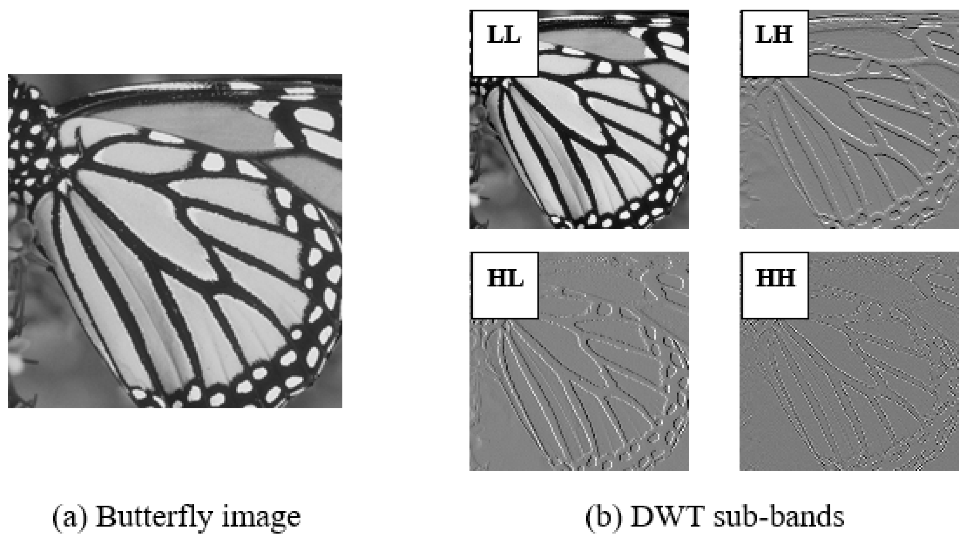
Image enlargement based on interpolation can be defined as the process of employing information from a small-sized image to generate a large-sized image by exploiting the correlation among neighboring pixels. Most image interpolation methods face two fundamental issues: (1) the involvement of errors and (2) image degradation during the enlargement process. The possible reason for these issues could be attributed to the fact that most of these methods similarly treat all image regions. Another reason could belong to the image-capturing process. This process involves sampling the source image into discrete points, which could result in losing some image information, particularly fine details. Theoretically, the interpolation process could not introduce new actual information into the image. Therefore, one of the possible solutions to address the previous issues is by introducing additional contextual information about the image. Most interpolation methods occur in the spatial domain. Therefore, any error would have a cumulative positive value, which is a possible reason for the first issue. Furthermore, these methods utilize relatively smooth functions that are incapable of reconstructing sharp edges and fine details, which is a possible cause for the second issue. On the other hand, when the image is processed in the spectral domain, any error would be distributed across the entire image region. Consequently, some errors may be less prominent at some points while being amplified at others. Ultimately, the final accumulated errors would be less in the spectral domain than in the spatial domain. The discrete wavelet transform (DWT) is a popular transformation that is employed to represent an image in the spectral domain. The DWT offers several useful features, such as multi-scale representation, sparsity representation, and adaptability. It has also been applied successfully in many image processing and computer vision problems, such as recognition [1,2,3], fusion [4], denoising [5], super-resolution [6], and edge detection [7]. The image is represented in this transform using four primary sub-bands. These sub-bands are denoted as LL, LH, HL, and HH. Figure 1 showcases the sub-bands obtained from applying the DWT to a butterfly image. From this figure, we can notice the relationship between the LL sub-band and the original image. This relationship can take the form of compression or expansion. In more detail, the LL sub-band can be employed to reconstruct a large-size version of the original image using the additional information contained in the remaining sub-bands (i.e., LH, HL, and HH) during the calculation of the inverse wavelet transform. If we assume that a low-size image represents the LL sub-band of a large-size image, the information in the remaining sub-bands should be provided to rebuild the large-size image. In this work, we use a simple edge detector to estimate the information in the LH, HL, and HH sub-bands. A list of contributions is given in the following points:

• This work introduces a simple method of interpolation for image enlargement based on edge detection and the DWT.
• The edge detection operators are exploited to estimate the information in the high-frequency sub-bands (i.e., LH, HL, and HH) of the DWT.
• The enlargement process is implemented by combining the first-order and second-order edge detectors with a small-sized image using the inverse wavelet transform to produce a large-sized image.
• Large-scale evaluations were applied on 20 different datasets, which were included in 11 databases comprising a total of 5500 different types of images, using the proposed work and the state-of-the-art work.

The remainder of the paper is organized as follows: Section 2 describes the mathematical equations and the principles of the DWT and edge detection. Section 3 depicts the important stages of the proposed enlargement process. Section 4 displays the important analyses and experiments. Finally, Section 5 summarizes the main findings of the experiments, the limitations of the current work, and the proposed future works.

2. Related Work

Several traditional interpolation algorithms are built for upscaling images, such as bilinear, bicubic, B-spline [8], and Lanczos [9]. Bilinear interpolates the values of the missing pixels using a linear function with four points. Bicubic interpolates the values using a cubic function with 16 points. B-spline implements interpolation using a piecewise curve. Lanczos uses a nonlinear sinc function to implement image interpolation. Two typical kernel sizes are used with Lanczos interpolation, which are 2 and 3. The main principle of these algorithms is to apply the convolution operation without regard to local region characteristics. To cope with the limitations of the traditional algorithms, several edge-guided image interpolation techniques that are related to the field of the proposed method are introduced. In ref. [10], a new edge-directed interpolation algorithm, namely NEDI, is developed. A hybrid scheme that combines bilinear and adaptive interpolation is implemented based on whether the current pixel represents an edge or not. Directional Filtering and Data Fusion are combined to develop a nonlinear interpolation algorithm [11]. The interpolation is implemented along two orthogonal directions using the neighborhood values of the missing pixels. The final value is obtained using linear minimum mean square estimation. An improved new edge direction (iNEDI) technique [12] has been developed to improve the quality of NEDI. This technique employed a dynamic window training size to cope with the sizes of the edges. However, the complexity of both algorithms is still high. Taylor series approximation is adopted in ref. [13] to calculate an interpolation process along four directions. For each point, four values are estimated and then combined to calculate a new interpolated value. The combination is adapted according to the orientation of a local edge. In ref. [14], the DWT and the discrete cosine transform (DCT) are integrated to build an interpolation algorithm for upscaling purposes. In this algorithm, the high-frequency components of the DWT are interpolated in the DCT. Aguerrebere, et al. [15] utilized a Gaussian mixture model (GMM) in a Bayesian framework for image restoration. The GMM was employed to model image patches. The proposed approach was adapted for missing data problems such as interpolation, zooming, and inpainting. An optimized image interpolation algorithm is suggested in refs. [16,17]. The interpolation process is implemented using the cubic trigonometric B-spline technique. The parameters of this technique are optimized using a genetic algorithm. Khalaf, et al. [18] introduced a new image interpolation algorithm to enhance the quality of JPEG compressed images. The algorithm starts by employing a smoothing filter to shrink and stretch images. A hyperbolic tangent function is then utilized to remove the effect of the resulting artifacts. A symmetric hyperbolic tangent function was then used as a curve-fitting function to overcome the blocking effects and edge degradation of the reconstructed image in ref. [19]. The discrete sine transform (DST) [20] is employed for image interpolation. A preprocessing step is implemented to obtain sharp interpolated images by upscaling and downscaling the LR image to calculate the error. The resulting error is added to the LR image. The algorithm called edge slope tracing (EST) is employed in ref. [21] for image interpolation. EST is utilized to predict the current slope from the adjacent slopes. To further improve the interpolation results, postprocessing operations, including two-way interpolation and thin edge correction, were used. In ref. [22], the interpolation of missing pixels in images is estimated using a rational bi-quartic spline algorithm with six parameters. Khan, et al. [23] utilized edge and gradient maps in image interpolation to reduce the effect of blurring and artifacts. An efficient hysteresis thresholding is introduced to build an edge map. Interpolation is then conducted on low-resolution edge maps to produce their corresponding high-resolution (HR) edge maps. In ref. [24], preprocessing steps are implemented before image interpolation to improve the quality of the reconstructed images. First, the unsharp mask is applied to a low-resolution (LR) image. Then, the blurred image is subtracted from the LR image to obtain a sharper image. Later, the resulting image is upscaled using the B-spline interpolation algorithm. Finally, the edges of the upscaled image are expanded to restore fine details. Regional gradient estimation is employed for edge detection in ref. [25]. A diffusion process is then applied to the detected edges. Next, the edge pixels are interpolated using a 1D directional filter, while the remaining pixels are interpolated using a directionless filter. The method in ref. [26] introduced a new interpolation algorithm for image upscaling using the hidden Markov model (HMM) and the hierarchical Dirichlet process (HDP). The HMM models the inter-scale dependencies of three consecutive levels of the DWT sub-bands of the LR image and its corresponding upscaled image, while the prior observation of the HMM is generated using the HDP. The proposed algorithm upscales images by a factor of 4. Spiking neural networks are employed in ref. [27] to detect image edges. A 1D directional filter is then utilized to interpolate edgy pixels, while the bicubic interpolation algorithm is utilized to interpolate the remaining pixels. A nonlinear scheme based on a pixel similarity technique is employed in ref. [28] to detect edges. Afterwards, a conditional interpolation process is implemented such that the edgy pixels are interpolated by applying 1D cubic interpolation and non-edgy pixels are interpolated by applying bicubic interpolation. A new postprocessing operation to mitigate the effect of blurring after image upscaling is implemented in ref. [29]. At the beginning, the primary interpolation operation is implemented using the Lanczos algorithm. Afterward, the edges of the interpolated image are highlighted using an adaptive sharpening process, and the smooth regions are smoothed using an anisotropic diffusion filter. To enhance the final interpolation results, residual-based restoration is implemented to enhance the quality of the undetected edges in the previous step. This technique involves many sophisticated operations. More related works use a lightweight approach termed fuzzy rough feature selection-based ANFIS interpolation (FRFS-ANFISI) [30] or use deep feature extraction modules for reconstruction networks based on feature reuse and structural reparameterization [31], or they utilize a multi-scale adaptive modulation network (MAMN), which mainly consists of a series of multi-scale adaptive modulation blocks (MAMBs). Each block combines a multi-scale adaptive modulation layer (MAML), a local detail extraction layer (LDEL), and two Swin Transformer Layers (STLs) [32]. Finally, more related works can be found in refs. [33,34,35]. All the described works are based on statistical and probabilistic techniques or deep learning models that involve several complex processes, which need many calculations to implement image interpolation. Consequently, the present work introduces a simple two-stage interpolation algorithm.

3. Mathematical Background

3.1. Discrete Wavelet Transform (DWT)

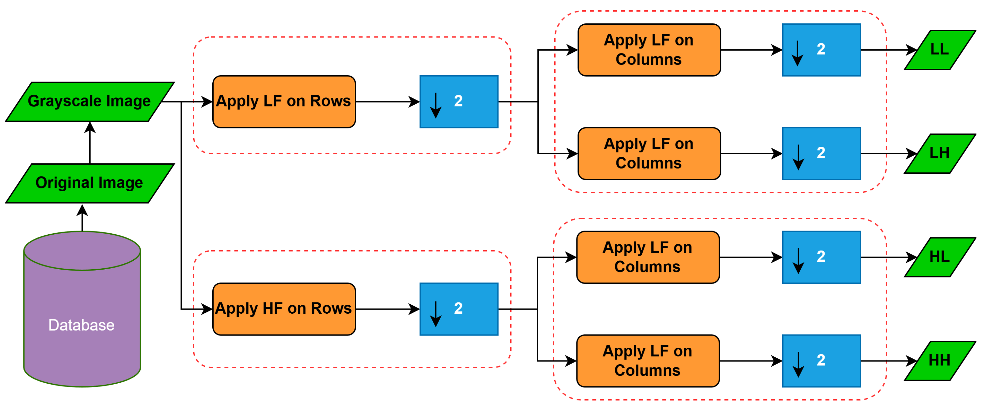
The DWT [36] provides a mathematical tool to manipulate signals at multiple resolutions. The DWT has several other useful properties, such as time and frequency localization, energy compactness, and sparse and hierarchical representation. The DWT can decompose digital images into approximate (low-frequency) and detailed (high-frequency) coefficients using two filters: high-pass (HF) and low-pass (LF). The result of 2D decomposition yields four sub-bands: LL, LH, HL, and HH. The low-frequency information is stored in the LL sub-band, while the high-frequency information is stored in the LH, HL, and HH sub-bands. These four sub-bands can be obtained by applying the LF and HF filters on image rows and columns as demonstrated in Figure 2.

As demonstrated in this figure, the size of the original image decreases to half when the LF and HF filters are applied to the image (the LF and HF filters could be applied on columns, then on rows, which makes no difference since the operation is reciprocal). The size of the resulting sub-bands is half that of the original image. The LF and HF coefficients are defined when the wavelet basis function (wavelet family) is determined. Several wavelet functions are available in the literature. Other wavelet functions were used, and the best wavelet function has been selected according to the best reported results, which were obtained using the Haar function. It is straightforward and computationally efficient. The coefficients of the LF and HF of the Haar wavelet function are given below.

$$LF={\displaystyle \frac{1}{2}}\left[\begin{array}{c}11\end{array}\right]$$

(1)

$$HF={\displaystyle \frac{1}{2}}\left[\begin{array}{c}1-1\end{array}\right]$$

(2)

In the case of digital images, it is essential that the values of 1/2 are used to ensure that the pixel values of the resulting image fall within the range of [0, 255]. The mathematical representations of the LL, LH, HL, and HH of the image using the 2D Haar filter are given below.

$$LL[i,j]={\displaystyle \frac{1}{4}}(F[i,2j]+F[i,2j+1]+F[2i,j]+F[2i+1,j])$$

(3)

$$LH[i,j]={\displaystyle \frac{1}{4}}(F[i,2j]+F[i,2j+1]-F[2i,j]-F[2i+1,j])$$

(4)

$$HL[i,j]={\displaystyle \frac{1}{4}}(F[i,2j]-F[i,2j+1]+F[2i,j]+F[2i+1,j])$$

(5)

$$HH[i,j]={\displaystyle \frac{1}{4}}(F[i,2j]-F[i,2j+1]-F[2i,j]-F[2i+1,j])$$

(6)

where F is a $2D$ image, $i=0,1,2,\dots R/2$, $j=0,1,2,\dots C/2$, and $R\times C$ is the image dimension.

3.2. First- and Second-Order Edge Detector

In this work, we derive simple first- and second-order edge detectors. The derivation is two-fold: (1) it should require a minimum number of mathematical operations and (2) it should be proportional to the type of the wavelet function. Besides, we adopt the Haar wavelet function due to its simplicity and efficiency, depending on the results of applying different wavelet functions. Figure 3 demonstrates the process of deriving the first-order (horizontal and vertical masks) and the second-order edge detector masks. In this figure, we assume that the white area is assigned a value of 1 and the black area is assigned a value of −1, while the value of 0 is assigned to the transition area (barrier) from black to white or vice versa.

The edge masks derived in Figure 3 represent the simplest form to estimate the image derivatives that involve a small number of mathematical operations. The horizontal edges are produced by convolving the image with the mask ${\partial }_y$, the vertical edges are produced by convolving the image with the mask ${\partial }_x$, while the second-order edges are obtained using the mask ${\partial }_x$${\partial }_y$. The values of the masks are given below.

$${\partial }_x={\displaystyle \frac{1}{2}}\left[\begin{array}{c}10-1\end{array}\right]$$

(7)

$${\partial }_y={\displaystyle \frac{1}{2}}\left[\begin{array}{c}\hfill 1\\ \hfill 0\\ \hfill -1\end{array}\right]$$

(8)

$${\partial }_x{\partial }_y={\displaystyle \frac{1}{4}}\left[\begin{array}{ccc}\hfill 1& \hfill 0& \hfill -1\\ \hfill 0& \hfill 0& \hfill 0\\ \hfill -1& \hfill 0& \hfill 1\end{array}\right]$$

(9)

3.3. Relationship Between DWT and Edge Detection

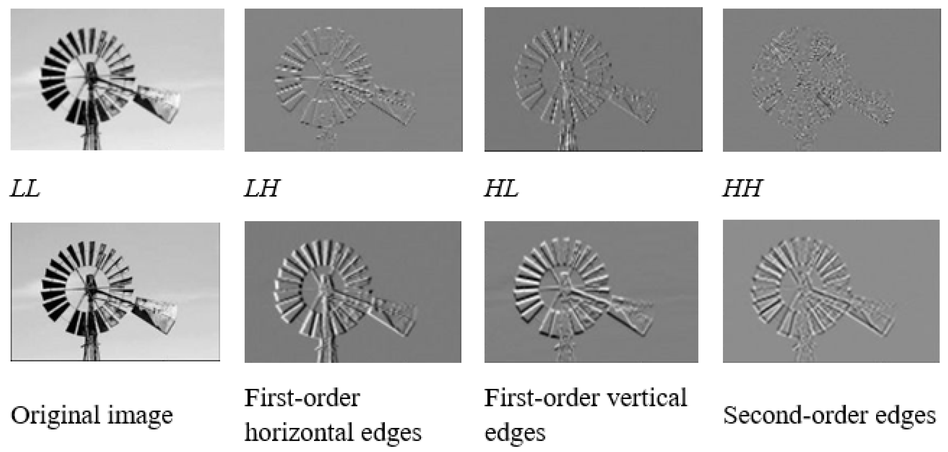
The relationship between the DWT sub-bands, namely the first-order and second-order image edge detectors, for instance, the Sobel filter, is shown in Figure 3. This figure displays the results of applying the first level of the 2D DWT (first row) and the results of edge detection using the first-order and second-order masks (second row).

The information in the LH sub-band highlights the values of the pixels at the horizontal edges, while the information in the HL sub-band highlights the values of the pixels at the vertical edges. On the other hand, the HH sub-band could be approximated when the horizontal and vertical edge detection masks are applied serially on images (second-order mask). The horizontal, vertical, and second-order edge detectors, derived in Section 3.2, are employed in this work to mimic the LH, HL, and HH sub-bands of the DWT. It should be emphasized that the edge detector masks are derived with respect to the Haar wavelet functions. However, applying these masks to the image alone can produce the information in the high-frequency sub-bands accurately as the Haar wavelet functions employ an implicit division factor of 4, whereas the proposed masks yield a maximum value of 2. Therefore, a normalization factor of 8 should be applied with the first-order masks and 64 with the second-order mask. Moreover, the process of enlargement to produce the SR image from the LR image involves two steps. The first step comprises applying masks ${\partial }_x$, ${\partial }_y$, and ${\partial }_v={\partial }_x$${\partial }_y$ separately on the LR image to estimate the approximate LH, HL, and HH sub-bands, respectively. This step can be described mathematically as

$$LH={\displaystyle \frac{{\partial }_x\otimes LR}{F}}$$

(10)

$$HL={\displaystyle \frac{{\partial }_y\otimes LR}{F}}$$

(11)

$$HH={\displaystyle \frac{{\partial }_v\otimes LR}{F^2}}$$

(12)

where ⊗ is the convolution operator, and $F$ is the normalization factor. The second step comprises the calculation of the inverse wavelet transform using the LR images and the estimated LH, HL, and HH sub-bands as follows:

$$M_{2i,2j}=L{R}_{i,j}+H{L}_{i,j}+L{H}_{i,j}+H{H}_{i,j}$$

(13)

$$M_{2i,2j+1}=L{R}_{i,j}+H{L}_{i,j}-L{H}_{i,j}-H{H}_{i,j}$$

(14)

$$M_{2i+1,2j}=L{R}_{i,j}-H{L}_{i,j}+L{H}_{i,j}-H{H}_{i,j}$$

(15)

$$M_{2i+1,2j+1}=L{R}_{i,j}-H{L}_{i,j}-L{H}_{i,j}+H{H}_{i,j}$$

(16)

where M is the HR image, and $i=0,1,2,\dots R-1$, $j=0,1,2,\dots C-1=0$, $R\times C$ is the size of the LR image.

4. Methodology

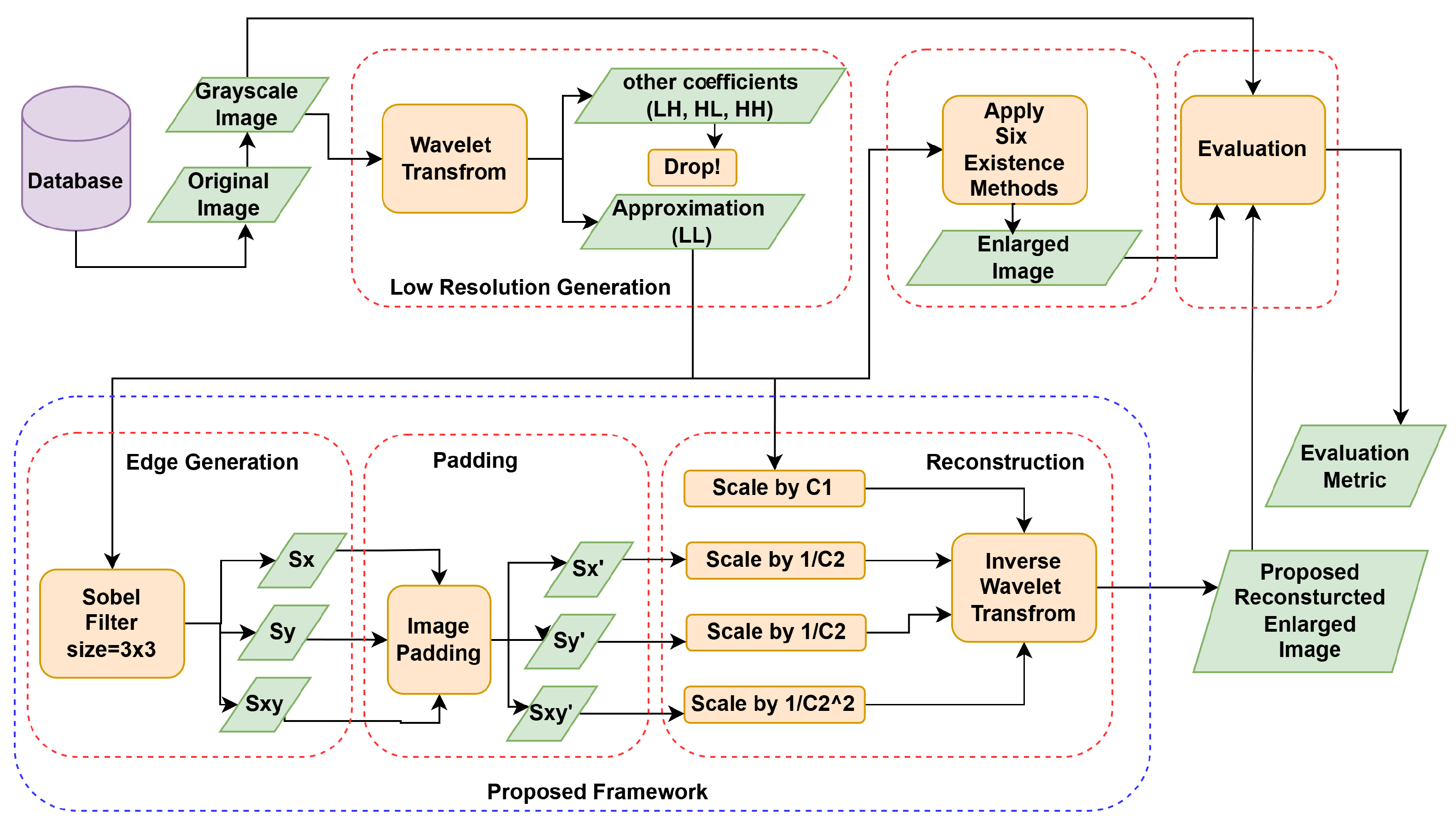
The proposed work in this paper consists of two preprocessing stages, which are image conversion and low-resolution generation. Moreover, there are four main stages, namely edge generation, image padding, image reconstruction, and the final evaluation, as shown in Figure 4.

4.1. Preprocessing

The preprocessing stage starts by converting the input image into a gray-level image, then generating a low-resolution image from the LL sub-band of the DWT; see Figure 4. Moreover, the other bands of the DWT were dropped since the proposed method is based on assuming that the $LR$ image (original) represents the LL sub-band of the DWT, while the corresponding super-resolution (SR) version can be built using the inverse DWT. The calculation of the inverse DWT requires the information in the four sub-bands of the DWT. Therefore, the missing information in the $LH$, $HL$, and $HH$ sub-bands should be provided. In this work, the mechanism of this scheme is aimed to mimic the information in the high-frequency sub-bands of the DWT using the first- and second-order edge detectors.

4.2. Proposed Work

The proposed method represents an enhanced version of the bilinear interpolation algorithm with the aim of recovering high-frequency information (e.g., edges and texture) using the inverse DWT. The first main stage in the proposed scheme is edge detection, as shown in Figure 4. In this stage, the Sobel filter of size $3\times 3$ is applied on the LL sub-band image of the DWT, which was obtained from preprocessing, since the LL sub-band represents the LR image. However, other filter sizes were used; the best fitter size was selected experimentally. Consequently, three images were obtained, namely Sx, Sy, and Sxy, which represent the horizontal direction, vertical direction, and diagonal direction edges, respectively. The size of the resulting images from the previous process is changed due to applying the mentioned filter. To address this issue, a padding operation is employed to produce the images Sx’, Sy’, and Sxy’. Moreover, the reconstruction process is implemented by scaling the LL sub-band by $C1=2$ factor and scaling the padded images Sx’ and Sy’ by $C2=4$ factor. Moreover, the Sxy’ image is scaled by ($1/C{2}^2$). In this trend, the resulting scaled images are applied to the inverse wavelet transform to produce the final reconstructed image. After that, the reconstructed (enlarged) image is evaluated with the original image using different image metrics, which are mentioned in the next section. Additionally, the original image is enlarged using the traditional interpolation methods, such as bilinear, bicubic, and Lanczos3, to compare the proposed work with the state-of-the-art works, as presented in the next section.

5. Results

The visual quality of the SR images produced by the proposed algorithm is assessed using some widely employed IQA metrics, such as mean squared error (MSE), peak signal-to-noise ratio (PSNR), and the structural similarity index (SSIM) [27,28,29]. On the other hand, edge-based IQA metrics such as gradient conduction mean square error (GCMSE) and non-shift edge-based ratio (NSER) are considered to measure the edge and structural properties of the resulting image [33].

The experiment was implemented on the 14 most frequently used images in the field of image interpolation (in addition to 20 datasets for which the results are shown at the end of this section), which are: Pepper ($256\times 256$), Baboon ($256\times 256$), Barbara ($512\times 512$), Boats ($512\times 512$), Cameraman ($256\times 256$), Airplane ($512\times 512$), House ($256\times 256$), Butterfly ($256\times 256$), Wheel ($512\times 512$), Fence ($768\times 512$), Bike ($232\times 348$), Stars ($183\times 275$), Lena ($512\times 512$), and Monarch ($512\times 768$) [20,24,26,27,28,29,33].

The MSE, GCMSE, and NSER are used to measure the quality of the proposed algorithm in comparison with traditional interpolation methods such as bilinear, bicubic, and Lanczo for scaling factor ($\times 2$), as shown in

Table 1. The ×2 results of MSE, GCMSE and NSER. Bold indicates the best; underline is the second-best.

ID	Image Name	Image Size	Metric	Proposed	Bilinear	Bicubic	Lanczos3
1	Pepper	256 × 256	MSE	55.043	77.408	55.92	53.316
			GCMSE	59.194	75.732	58.617	57.058
			NSER	0.910	0.891	0.906	0.909
2	Baboon	256 × 256	MSE	131.936	162.999	138.12	136.685
			GCMSE	33.619	43.282	37.311	36.581
			NSER	0.881	0.863	0.876	0.877
3	Barbara	512 × 512	MSE	172.589	202.075	186.143	189.704
			GCMSE	764.877	829.103	836.275	863.727
			NSER	0.839	0.804	0.824	0.825
4	Boats	512 × 512	MSE	59.64	80.701	61.053	59.17
			GCMSE	271.342	374.217	283.976	273.114
			NSER	0.912	0.897	0.910	0.911
5	Cameraman	256 × 256	MSE	200.575	255.824	207.811	204.051
			GCMSE	538.856	675.385	565.806	554.041
			NSER	0.888	0.868	0.882	0.883
6	Airplane	512 × 512	MSE	45.456	63.247	44.006	42.494
			GCMSE	267.767	299.926	242.888	240.487
			NSER	0.915	0.899	0.913	0.914
7	House	256 × 256	MSE	51.815	65.914	51.472	51.216
			GCMSE	68.486	75.121	61.816	62.203
			NSER	0.895	0.879	0.888	0.886
8	Butterfly	256 × 256	MSE	136.174	217.243	139.053	130.794
			GCMSE	130.591	176.805	117.299	113.912
			NSER	0.931	0.904	0.927	0.932
9	Wheel	512 × 512	MSE	448.587	555.676	467.884	463.535
			GCMSE	4151.25	5159.393	4394.124	4338.737
			NSER	0.878	0.855	0.870	0.872
10	Fence	768 × 512	MSE	105.76	136.976	110.682	108.349
			GCMSE	590.768	790.84	625.268	605.346
			NSER	0.893	0.879	0.891	0.893
11	Bike	232 × 348	MSE	176.495	237.406	181.881	176.896
			GCMSE	184.272	240.511	191.617	187.087
			NSER	0.911	0.892	0.908	0.910
12	Stars	183 × 275	MSE	181.899	242.796	189.275	185.075
			GCMSE	329.113	412.421	334.661	328.005
			NSER	0.909	0.886	0.903	0.907
13	Lena	512 × 512	MSE	26.300	39.041	26.808	25.454
			GCMSE	64.099	89.086	56.507	53.897
			NSER	0.935	0.913	0.933	0.937
14	Monarch	512 × 768	MSE	38.284	61.625	39.021	36.567
			GCMSE	658.228	910.622	600.864	578.999
			NSER	0.934	0.908	0.93	0.935
Average MSE				130.754	171.352	135.652	133.093
Average GCMSE				579.462	725.175	600.502	592.371
Average NSER				0.902	0.881	0.897	0.899

. For the MSE results, the proposed method averaged $130.753$, whereas the bilinear, bicubic, and Lanczo methods averaged $171.352$, $135.652$, and $133.093$, respectively. For the GCMSE, which is a modified version of MSE that measures the difference between the edge and non-edge pixels, the proposed method averaged $579.461$, whereas the bilinear, bicubic, and Lanczo methods averaged $725.175$, $600.502$, and $592.371$, respectively. For the NSER results, the proposed method averaged $0.902404$, whereas the bilinear, bicubic, and Lanczo methods averaged $0.881404$, $0.897188$, and $0.899436$, respectively. The output images using the proposed method mostly yield either the best or second-best for the MSE, GCMSE, and NSER metrics for every single image. The high NSER value for most of the test images using the proposed method certainly highlights the ability of the proposed algorithm to be reasonably compatible across the board. The Lanczos method produces comparable MSE and GCMSE for some images because of its function, which has some malformation effect on the edges.

Table 2. The ×4 results of MSE, GCMSE, and NSER. Bold is the best; underline is the second-best.

ID	Image Name	Image Size	Metric	Proposed	Bilinear	Bicubic	Lanczos3
1	Pepper	256 × 256	MSE	170.227	242.505	173.551	168.408
			GCMSE	130.148	145.524	129.832	127.519
			NSER	0.68	0.646	0.656	0.668
2	Baboon	256 × 256	MSE	264.868	307.184	271.191	269.211
			GCMSE	60.088	62.325	61.216	60.977
			NSER	0.662	0.642	0.657	0.661
3	Barbara	512 × 512	MSE	278.219	314.13	281.094	278.685
			GCMSE	915.300	927.438	919.082	918.801
			NSER	0.587	0.56175	0.582	0.591
4	Boats	512 × 512	MSE	172.02	219.989	178.118	175.484
			GCMSE	631.393	718.339	653.725	643.355
			NSER	0.693	0.6675	0.674	0.678
5	Cameraman	256 × 256	MSE	459.309	558.434	473.546	469.411
			GCMSE	971.002	1038.102	997.438	991.507
			NSER	0.661	0.616	0.626	0.633
6	Airplane	512 × 512	MSE	146.523	201.999	149.562	146.268
			GCMSE	525.075	566.199	509.145	506.059
			NSER	0.681	0.663	0.67	0.677
7	House	256 × 256	MSE	140.811	189.492	140.651	137.297
			GCMSE	124.749	136.362	120.682	120.122
			NSER	0.652	0.638	0.644	0.650
8	Butterfly	256× 256	MSE	499.735	760.644	510.891	495.950
			GCMSE	328.854	387.509	316.901	310.568
			NSER	0.701	0.636	0.654	0.663
9	Wheel	512 × 512	MSE	918.359	1082.018	939.687	931.865
			GCMSE	7014.315	7966.385	7267.618	7204.739
			NSER	0.656	0.618	0.626	0.629
10	Fence	768 × 512	MSE	275.759	317.858	286.958	287.475
			GCMSE	1367.616	1477.285	1415.000	1414.097
			NSER	0.609	0.581	0.587	0.590
11	Bike	232 × 348	MSE	451.693	577.965	462.939	454.911
			GCMSE	360.097	407.412	365.891	361.537
			NSER	0.691	0.674	0.682	0.685
12	Stars	183 × 275	MSE	460.101	593.359	473.02	466.248
			GCMSE	625.459	688.218	630.015	623.350
			NSER	0.680	0.639	0.651	0.654
13	Lena	512 × 512	MSE	83.704	120.095	86.298	84.030
			GCMSE	179.415	208.997	171.827	169.264
			NSER	0.713	0.670	0.693	0.705
14	Monarch	512 × 768	MSE	143.758	220.12	147.001	142.986
			GCMSE	1713.510	2010.890	1659.277	1630.07
			NSER	0.707	0.647	0.669	0.676
Average MSE				318.935	407.556	326.751	322.016
Average GCMSE				1067.644	1195.785	1086.975	1077.283
Average NSER				0.670	0.636	0.648	0.654

shows the results of these metrics, but this time for scaling factor $\times 4$. Similarly, the averaged results of the proposed algorithm are better than the results of bilinear, bicubic, and Lanczo interpolation. The high NSER value of the proposed method indicates that the image quality is the best for human visual perception also with scaling factor $\times 4$, especially in terms of edge perception.

Furthermore, PSNR and SSIM are employed to evaluate the quality of the resulting images against selected references [19,24,26,27,28,33,37].

Table 3. The PSNR and SSIM results of the proposed method compared to different methods (the bolded values are the best, whereas the underlined values are the second-best).

ID	Image Name	Size	Proposed	Ref. [24]	Ref. [23]	Ref. [25]	Ref. [17]	Ref. [21] (GEI)	Ref. [30]	Ref. [34]
1	Pepper	256 × 256	34.949	31.120	32.210	33.350	35.540	30.810	34.886	27.820
			0.973	0.928	0.878	0.939	0.968	0.903	0.891	0.890
2	Baboon	256 × 256	30.936	22.82	23.29	23.54	26.46	22.59	29.831	27.77
			0.857	0.940	0.689	0.971	0.817	0.917	0.714	0.74
3	Barbara	512 × 512	32.616	24.25		24.93		24.01	32.465	32.860
			0.868	0.939		0.970		0.912	0.836	0.85
4	Boats	512 × 512	33.562	29.71	33.160	32.05		29.42
			0.916	0.896	0.871	0.919		0.879
5	Cameraman	256 × 256	32.891	26.09	26.34	27.040		25.83
			0.895	0.898	0.782	0.948		0.873
6	Airplane	512 × 512	35.987	26.88	35.520	28.54		26.61
			0.965	0.959	0.946	0.968		0.941
7	House	256 × 256	34.970	33.170		35.380		32.840
			0.922	0.896		0.899		0.878
8	Butterfly	256 × 256	32.352	29.55	30.2	30.96		29.26	32.284	28.06
			0.963	0.999	0.942	0.998		0.976	0.905	0.780
9	Wheel	512 × 512	31.373	21.53		22.530		21.32
			0.859	0.899		0.909		0.867
10	Fence	768 × 512	32.871	26.01		27.830		25.75
			0.897	0.789		0.812		0.772
11	Bike	232 × 348	31.090	26.6		27.380		25.85
			0.913	0.907		0.921		0.879
12	Stars	183 × 275	34.293	34.670		37.450		34.33
			0.951	0.976		0.998		0.961
13	Lena	512 × 512	35.535		34.25		35.270		34.854	34.9
			0.932		0.914		0.957		0.899	0.91
14	Monarch	512 × 768	36.946		30.99		36.08		36.373	27.46
			0.976		0.874		0.965		0.952	0.95

displays the comparison results of the proposed algorithm with these references in terms of PSNR and SSIM. For 10 out of the 14 test images, the proposed method achieves the highest PSNR values, while, for three images of the remaining four, it attains the second-highest PSNR. These results indicate that the proposed algorithm can be considered as a competitive approach in terms of minimum noise production and good image edge preservation.

To provide a broader evaluation, in addition to the commonly used standard benchmark test images, we applied our proposed method on some datasets with diverse characteristics that are widely utilized in image interpolation and high-resolution research, which are: Set5, Set14, BSD100, and Urban100. They were compared with the most applicable interpolation techniques, which are bilinear and bicubic methods, and some state-of-the-art image super-resolution reconstruction methods, including ANFIS $KAZ{E}_{P}S{O}_{4}1$ [30], FS2R-L [31], MAMN [32], MOION [34], and MADNet [35], by objective evaluation metrics (PSNR and SSIM).

Table 4. PSNR and SSIM comparison with other references for different datasets (×2).

Dataset	Bilinear	Bicubic	Ref. [32]	Ref. [31]	Ref. [29]	Ref. [28]	Ref. [27]	Proposed
			MADNet	MOION	MAMN	FS2R-L	ANFIS
Set 5	34.304	35.200	37.850	38.160	38.120	37.790	35.120	35.343
	0.941	0.959	0.960	0.962	0.961	0.963	0.952	0.962
Set 14	32.819	33.321	33.380	33.920	33.810	33.300	30.810	33.498
	0.881	0.913	0.916	0.920	0.919	0.922	0.906	0.921
BSD100	32.617	33.027	32.040	32.320	32.280	31.907	30.840	33.168
	0.901	0.852	0.8979	0.901	0.901	0.906	0.886	0.892
Urban100	32.119	32.344	31.620	32.690	32.360	31.220	28.830	32.535
	0.856	0.892	0.923	0.934	0.930	0.924	0.892	0.903

displays the comparison of the reconstruction results for scaling factor ×2.

From Table 4, the results demonstrate that the proposed method is strongly competitive on the BSD100 dataset and achieves the second-highest PSNR value on the Urban100 dataset. Furthermore, the proposed method obtains the second-best SSIM value on both Set5 and Set14 datasets, although it maintains low computational complexity. On the other hand,

Table 5. PSNR and SSIM comparison with other references for different datasets (×4).

Dataset	Bilinear	Bicubic	Ref. [32]	Ref. [31]	Ref. [29]	Ref. [28]	Ref. [27]	Proposed
			MADNet	MOION	MAMN	FS2R-L	ANFIS
Set 5	31.526	32.338	31.95	32.51	32.35	32.01		32.478
	0.818	0.877	0.8917	0.898	0.896	0.902		0.885
Set 14	30.974	31.451	28.44	28.85	28.81	28.56		31.572
	0.713	0.7819	0.778	0.788	0.786	0.797		0.798
BSDS100	31.102	31.458	27.47	27.72	27.7	27.55		31.539
	0.667	0.736	0.7327	0.742	0.739	0.753		0.755
Urban100	30.617	30.968	25.76	26.55	26.39	25.87		31.066
	0.672	0.743	0.775	0.801	0.793	0.792		0.762

displays a comparison of reconstruction results for a scaling factor of ×4. The proposed method outperforms both traditional interpolation techniques and state-of-the-art methods in terms of the PSNR metric on the Set14, BSD100, and Urban100 datasets and achieves the second-highest value on the Set5 dataset. Moreover, the proposed method obtains the highest SSIM value for Set14 and BSD100 and the second-highest value on the Set5 dataset, which indicates good preservation of image edges with minimal structural loss.

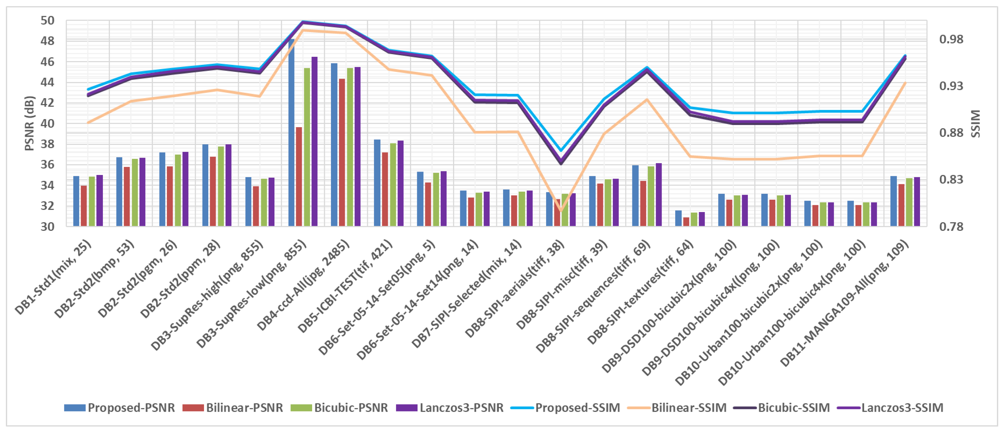
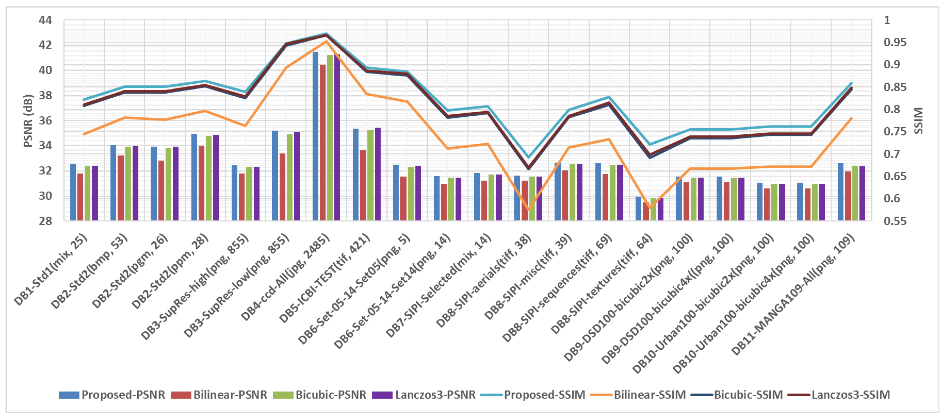
Moreover, an additional evaluation is conducted on 20 datasets included in the 11 databases with an overall 5500 images. The evaluation uses two main metrics, namely PSNR and SSIM, for ×2 results, as shown in Figure 5.

Moreover, an additional evaluation is conducted on 20 datasets included in the 11 overall databases. The evaluation uses two main metrics, namely PSNR and SSIM, for ×4 results, as shown in Figure 6. The reported results for ×2 and ×4 show the superiority of the proposed work over the existence methods.

6. Discussion

The quality of the proposed interpolation algorithm is compared to that of its counterparts (bilinear, bicubic, and Lanczos3). It can be observed that the proposed algorithm produces superior visual quality compared to traditional interpolation methods (bilinear, bicubic, and Lanczos3). The possible reasons for these results are: (1) we employed simple steps to estimate the high-frequency sub-bands of the DWT and (2) we utilized the Haar wavelet, which is one of the simplest functions, in the reconstruction process. By employing more advanced techniques and sophisticated wavelet functions, the results of the interpolation would be improved. The importance of the proposed algorithm is highlighted in

Table 6. The total cost of interpolation algorithms.

Method	Add/Sub	Shift	Mult/Div	Sin	Total Cost in Clock Cycles	Rational Cost
Bilinear	4	4	0	0	64	1
Bicubic	57	22	47	0	6836	106.8
Lancsoz3	47	32	86	24	539,984	8437
Proposed	11	3	0	0	112	1.75

, which demonstrates the computational cost of each algorithm. First, the computational cost of each mathematical and logical operation per pixel is estimated. The approximate cost is calculated by determining the number of cycles required to complete each operation, i.e., latency (in clock cycles). To calculate the total cost of the clock cycle, the addition and subtraction (Add/Sub) require eight clocks. The shift operation (equivalent to multiplication or division by a power of 2) requires eight clocks. The multiplication and division require 64–200 clocks (average 132 clocks). The complex sine function requires approximately 14,925–29,344 clocks (an average of 22,000 clocks) [38,39]. To simplify the comparison, the cost of the bilinear method, which is the cheapest one, is considered equal to 1, and then the rational cost is recalculated for the other methods, as listed in the last column of Table 6.

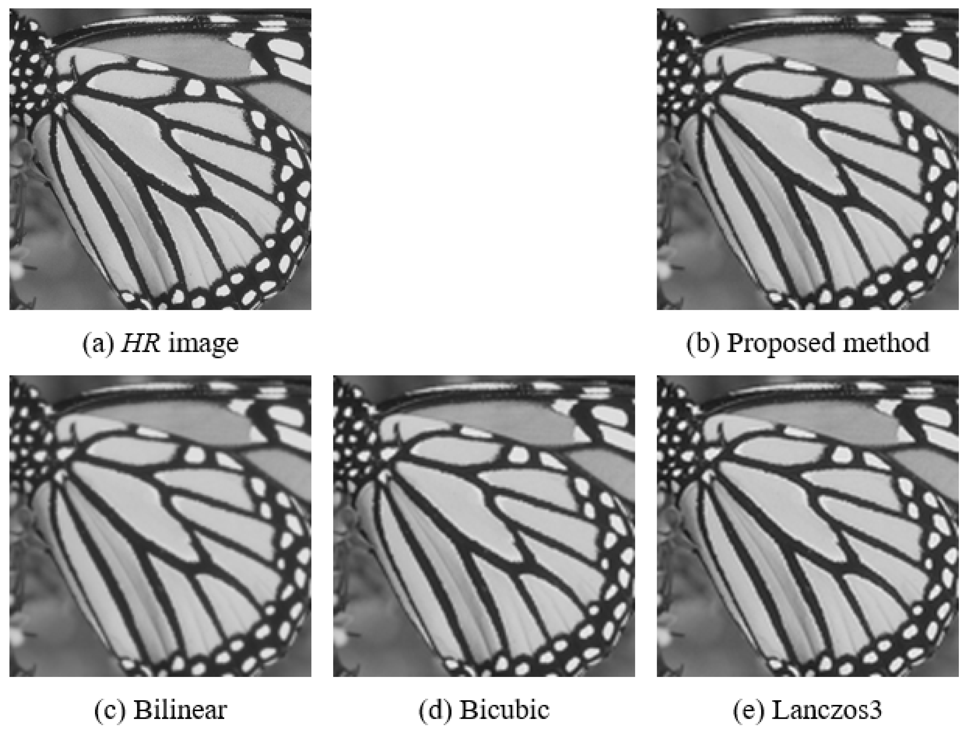
As shown in Table 6, the bilinear algorithm has the lowest cost, while its reconstruction quality is modest. Our proposed algorithm has the second-lowest cost. Meanwhile, the Lanczos3 algorithm has the highest cost. From Table 1 and Table 2 the results show that there are two choices. The first choice is to utilize traditional methods, which are simple, easy to implement, and used in many applications. The second choice is to utilize complicated and cost-effective methods, such as Lanczos, to obtain good results, but they may not be suitable for real-time implementation. This is because these methods deal with the image as data (numerical values and discrete functions), not as information carried on some data. In this article, a new perspective for dealing with an image as a group of information, not as a group of data, is proposed to enhance images. Using the wavelet transform as an enlargement tool is the key development of this work, which generated some algorithms with different efficiencies and complexities in comparison with previous works. In summary, this work focuses on enlarging images using a straightforward algorithm that employs the Haar filter with a one-level 2D wavelet transform to increase image size by a factor of 2 and two-level 2D to increase image size by a factor of 4. Although this algorithm has its limitations, it offers a simple approach for image enlargement. Its performance is comparable to traditional methods in terms of complexity and to advanced methods regarding result quality. Our new insights involve developing advanced algorithms that utilize more complex wavelet families, such as Daubchies 4 and 8, and implementing a multi-level 2D wavelet transform. Figure 7 displays the output images using different interpolation algorithms. The output image from the bilinear interpolation algorithm has the lowest visual quality with a more blurred effect. The other algorithms produce better visual quality.

7. Conclusions

A new image interpolation technique based on edge detection and a wavelet transform for image enlargement has been introduced. Wavelet transforms provide a way to decompose an image into multiple frequency sub-bands, enabling a clear separation between high-frequency components, such as edges and details, and low-frequency components, such as uniform and smooth regions. This decomposition is important for reconstructing images with high quality. By leveraging edge detection algorithms to estimate the high-frequency components, this method identifies and preserves important details and sharp transitions within the image, which is crucial for improving visual quality and preserving edges during the inverse wavelet transform. The proposed method, with its simplicity, exceeded some of the standard methods in quality for the enlarged image, like bilinear and bicubic interpolation methods, and reduced the computation time by more than 4800 times for the Lanczos3 method. The reported results show outstanding differences between the proposed method and the existing methods (bilinear, bicubic, and Lanczos3, respectively) for x4 enlargement, in which the obtained average MSEs are 89, 8, and 4. Also, the average GCMSEs are 128, 19, and 10. Moreover, the average NSERs are 0.034, 0.022, and 0.016.

The main limitation of the current work is that it is designed to work with the Haar wavelet transform. The work is ongoing to optimize the edge detectors and explore improved wavelet techniques to boost the overall performance across diverse image types. For future work, other image techniques, such as 3D reconstruction, extrapolation, and interpolation filtering, will be involved.

References

1. Abdulsattar, F.S. On the Effectiveness of Using Wavelet-based LBP Features for Melanoma Recognition in Dermoscopic Images. In Proceedings of the 2021 International Conference on Information Technology (ICIT); IEEE: New York, NY, USA, 2021; pp. 406–411. [Google Scholar]
2. Liu, Y.; Wang, C.; Lu, M.; Yang, J.; Gui, J.; Zhang, S. From simple to complex scenes: Learning robust feature representations for accurate human parsing. IEEE Trans. Pattern Anal. Mach. Intell. 2024, 46, 5449–5462. [Google Scholar] [CrossRef] [Scilit] [PubMed]
3. Wang, S.; Wang, C.; Shi, C.; Liu, Y.; Lu, M. Mask-guided mamba fusion for drone-based visible-infrared vehicle detection. IEEE Trans. Geosci. Remote Sens. 2024, 62, 5005712. [Google Scholar] [CrossRef] [Scilit]
4. Gebremeskel, G.B. A critical analysis of the multi-focus image fusion using discrete wavelet transform and computer vision: GB Gebremeskel. Soft Comput. 2022, 26, 5209–5225. [Google Scholar] [CrossRef] [Scilit]
5. Tian, C.; Zheng, M.; Zuo, W.; Zhang, B.; Zhang, Y.; Zhang, D. Multi-stage image denoising with the wavelet transform. Pattern Recognit. 2023, 134, 109050. [Google Scholar] [CrossRef] [Scilit]
6. Yu, Y.; She, K.; Liu, J.; Cai, X.; Shi, K.; Kwon, O.M. A super-resolution network for medical imaging via transformation analysis of wavelet multi-resolution. Neural Netw. 2023, 166, 162–173. [Google Scholar] [CrossRef] [Scilit] [PubMed]
7. Fujinoki, K.; Ashizawa, K. Directional lifting wavelet transform for image edge analysis. Signal Process. 2024, 216, 109188. [Google Scholar] [CrossRef] [Scilit]
8. Xia, P.; Tahara, T.; Kakue, T.; Awatsuji, Y.; Nishio, K.; Ura, S.; Kubota, T.; Matoba, O. Performance comparison of bilinear interpolation, bicubic interpolation, and B-spline interpolation in parallel phase-shifting digital holography. Opt. Rev. 2013, 20, 193–197. [Google Scholar] [CrossRef] [Scilit]
9. He, L.; Wu, H.; Zhao, X. The application of Lanczos interpolation in video scaling system based on FPGA. In Proceedings of the Twelfth International Conference on Signal Processing Systems; SPIE: Bellingham, WA, USA, 2021; Volume 11719, pp. 120–126. [Google Scholar]
10. Li, X.; Orchard, M.T. New edge-directed interpolation. IEEE Trans. Image Process. 2001, 10, 1521–1527. [Google Scholar] [CrossRef] [Scilit] [PubMed]
11. Zhang, L.; Wu, X. An edge-guided image interpolation algorithm via directional filtering and data fusion. IEEE Trans. Image Process. 2006, 15, 2226–2238. [Google Scholar] [CrossRef] [Scilit] [PubMed]
12. Asuni, N.; Giachetti, A. Accuracy improvements and artifacts removal in edge based image interpolation. In Proceedings of the International Conference on Computer Vision Theory and Applications; SciTePress: Setubal, Portugal, 2008; Volume 2, pp. 58–65. [Google Scholar]
13. Lee, S.J.; Kang, M.C.; Uhm, K.H.; Ko, S.J. An edge-guided image interpolation method using Taylor series approximation. IEEE Trans. Consum. Electron. 2016, 62, 159–165. [Google Scholar] [CrossRef] [Scilit]
14. Lama, R.K.; Shin, S.; Kang, M.; Kwon, G.R.; Choi, M.R. Interpolation using wavelet transform and discrete cosine transform for high resolution display. In Proceedings of the 2016 IEEE International Conference on Consumer Electronics (ICCE); IEEE: New York, NY, USA, 2016; pp. 184–186. [Google Scholar]
15. Aguerrebere, C.; Almansa, A.; Delon, J.; Gousseau, Y.; Musé, P. A Bayesian hyperprior approach for joint image denoising and interpolation, with an application to HDR imaging. IEEE Trans. Comput. Imaging 2017, 3, 633–646. [Google Scholar] [CrossRef] [Scilit]
16. Abbas, S.; Irshad, M.; Hussain, M.Z. Adaptive image interpolation technique based on cubic trigonometric B-spline representation. IET Image Process. 2018, 12, 769–777. [Google Scholar] [CrossRef] [Scilit]
17. Al-Rifaee, Z.I.A.; Mohammed, S.A.; Abood, S.I. Upscale Gray Image using Mixing Transform Generation based on Tensor Product. J. Inf. Hiding Multimed. Signal Process. 2025, 16, 379–388. [Google Scholar]
18. Khalaf, W.; Al Gburi, A.; Zaghar, D. Pre and postprocessing for JPEG to handle large monochrome images. Algorithms 2019, 12, 255. [Google Scholar] [CrossRef] [Scilit]
19. Khalaf, W.; Zaghar, D.; Hashim, N. Enhancement of curve-fitting image compression using hyperbolic function. Symmetry 2019, 11, 291. [Google Scholar] [CrossRef] [Scilit]
20. Panda, J.; Meher, S. A novel approach of image interpolation using DST. In Proceedings of the 2019 Fifth International Conference on Image Information Processing (ICIIP); IEEE: New York, NY, USA, 2019; pp. 606–611. [Google Scholar]
21. Khan, S.; Lee, D.H.; Khan, M.A.; Gilal, A.R.; Mujtaba, G. Efficient edge-based image interpolation method using neighboring slope information. IEEE Access 2019, 7, 133539–133548. [Google Scholar] [CrossRef] [Scilit]
22. Karim, S.A.A. Rational bi-quartic spline with six parameters for surface interpolation with application in image enlargement. IEEE Access 2020, 8, 115621–115633. [Google Scholar] [CrossRef] [Scilit]
23. Khan, S.; Lee, D.H.; Khan, M.A.; Siddiqui, M.F.; Zafar, R.F.; Memon, K.H.; Mujtaba, G. Image Interpolation via Gradient Correlation-Based Edge Direction Estimation. Sci. Program. 2020, 2020, 5763837. [Google Scholar] [CrossRef] [Scilit]
24. Jia, Z.; Huang, Q. Image interpolation with regional gradient estimation. Appl. Sci. 2022, 12, 7359. [Google Scholar] [CrossRef] [Scilit]
25. Panda, J.; Meher, S. An improved image interpolation technique using OLA e-spline. Egypt. Inform. J. 2022, 23, 159–172. [Google Scholar] [CrossRef] [Scilit]
26. Khalili Sadaghiani, A.; Forouzandeh, B. Image interpolation based on 2D-DWT and HDP-HMM. Pattern Anal. Appl. 2022, 25, 361–377. [Google Scholar] [CrossRef] [Scilit]
27. İncetaş, M.O. Image interpolation based on spiking neural network model. Appl. Sci. 2023, 13, 2438. [Google Scholar] [CrossRef] [Scilit]
28. Kılıçaslan, M. Image interpolation with spiking neural network based pixel similarity. Signal Image Video Process. 2024, 18, 6925–6936. [Google Scholar] [CrossRef] [Scilit]
29. Panda, J.; Meher, S. An improved method for upscaling 2D images using adaptive edge sharpening and an optimized directional anisotropic diffusion filter. Eng. Appl. Artif. Intell. 2024, 136, 109045. [Google Scholar] [CrossRef] [Scilit]
30. Ismail, M.; Shang, C.; Yang, J.; Shen, Q. Supporting ANFIS interpolation for image super resolution with fuzzy rough feature selection. Appl. Intell. 2024, 54, 5373–5388. [Google Scholar] [CrossRef] [Scilit]
31. Li, T.; Jin, X.; Liu, Q.; Liu, X. Image Super-Resolution Reconstruction Network Based on Structural Reparameterization and Feature Reuse. Sensors 2025, 25, 5989. [Google Scholar] [CrossRef] [Scilit] [PubMed]
32. Liu, Z.; Zhang, G.; Tian, J.; Qi, R. Multi-Scale Adaptive Modulation Network for Efficient Image Super-Resolution. Electronics 2025, 14, 4404. [Google Scholar] [CrossRef] [Scilit]
33. Nor Azam, N.Z.F.; Yazid, H.; Abdul Rahim, S. Single image super-resolution using Gabor response-weighted interpolation. Imaging Sci. J. 2025, 73, 918–932. [Google Scholar] [CrossRef] [Scilit]
34. Gao, S.; Li, L.; Cui, W.; Jiang, H.; Ge, H. Lightweight image super-resolution reconstruction network based on multi-order information optimization. Sensors 2025, 25, 5275. [Google Scholar] [CrossRef] [Scilit] [PubMed]
35. Lan, R.; Sun, L.; Liu, Z.; Lu, H.; Pang, C.; Luo, X. MADNet: A fast and lightweight network for single-image super resolution. IEEE Trans. Cybern. 2020, 51, 1443–1453. [Google Scholar] [CrossRef] [Scilit] [PubMed]
36. Mallat, S.G. A theory for multiresolution signal decomposition: The wavelet representation. IEEE Trans. Pattern Anal. Mach. Intell. 2002, 11, 674–693. [Google Scholar]
37. Arezoomand, A.; Cheraaqee, P.; Mansouri, A. Perceptually optimized loss function for image super-resolution. In Proceedings of the 2021 7th International Conference on Signal Processing and Intelligent Systems (ICSPIS); IEEE: New York, NY, USA, 2021; pp. 1–5. [Google Scholar]
38. Suresh, C.; Singh, S.; Saini, R.; Saini, A.K. A comparative analysis of image scaling algorithms. Int. J. Image Graph. Signal Process. 2013, 5, 55. [Google Scholar] [CrossRef] [Scilit]
39. Faz-Hernández, A.; Fujii, H.; Aranha, D.F.; López, J. A secure and efficient implementation of the quotient digital signature algorithm (qDSA). In Proceedings of the International Conference on Security, Privacy, and Applied Cryptography Engineering; Springer: Berlin/Heidelberg, Germany, 2017; pp. 170–189. [Google Scholar]
Figure 1. The decomposition of a butterfly image into four sub-bands using the DWT.
Digital 06 00064 g001
Figure 2. The 2D decomposition of an image into four sub-bands using the DWT, where LF and HF denote low-pass and high-pass filters and 2 denotes downsampling by 2.
Digital 06 00064 g002
Figure 3. The relationship between the DWT and edge detection.
Digital 06 00064 g003
Figure 4. The overall processes of the proposed work.
Digital 06 00064 g004
Figure 5. The result of ×2 on different datasets using PSNR and SSIM.
Digital 06 00064 g005
Figure 6. The result of ×4 on different datasets using PSNR and SSIM.
Digital 06 00064 g006
Figure 7. The HR image using different interpolation algorithms.
Digital 06 00064 g007