Article

Raman Spectroscopy of Protein–Polysaccharide Conjugates: A Comparative Study of Tree-Based Ensemble Models


by
Svetlana A. Shevtsova
1,
Samvel A. Grigoryan
2,
Oksana A. Mayorova
1,
Mariia S. Saveleva
1 and
Ekaterina S. Prikhozhdenko
2,*
1
Science Medical Center, Saratov State University, 83 Astrakhanskaya Str., 410012 Saratov, Russia
2
Future Biophysics Institute, Moscow Center for Advanced Studies, 20 Kulakova Str., 141700 Moscow, Russia
*
Author to whom correspondence should be addressed.
Macromol 2026, 6(2), 37; https://doi.org/10.3390/macromol6020037

Submission received: 25 November 2025 / Revised: 30 March 2026 / Accepted: 1 June 2026 / Published: 3 June 2026

Abstract

Proteins with additives, especially in small quantities, are of great interest as a subject of study. Machine learning approaches implemented on Raman spectroscopy data could provide an insight into the chemical structures of such mixtures or conjugates. Although decision tree models could be powerful in solving either classification or regression tasks and could provide accessible predictions, they are prone to overfitting. Ensemble models that implement several decision trees could overcome the determined problem. Five different model types are discussed: RandomForest, GradientBoosting, AdaBoost, Voting, and Stacking. Raman spectroscopy data of whey protein isolates (5 wt.%) with different amounts of hyaluronic acid (0, 0.1, 0.25, and 0.5 wt.%) were used as datasets. In order to generalize the results of the study, WPI samples from three different manufacturers were used. Optimization established that ensembles of 200 decision trees with a maximum depth of four were optimal. The Stacking algorithm, which used RandomForest, GradientBoosting, and AdaBoost as base models with either LogisticRegressor (classification task) or RidgeCV (regression task), was found to be the most efficient in finding differences between the whey protein isolate and its conjugates with hyaluronic acid: specificity of 68.7% and sensitivity of 95.4% (classification task); R2 = 0.764 with mean absolute error of 0.068 (regression task). According to the feature importance plots, the Raman bands that were most influential in predicting the results were 1003 cm−1 (phenylalanine, ring breath), 1125 cm−1 (rocking of NH3+), 1206 cm−1 (C–C stretching), 1240 cm−1 (amide III (β-sheet), N–H in-plane bend, C–N stretch), and 1399 cm−1 (aspartic and glutamic acids, C=O stretch of COO–). The findings of this study may contribute to the development of novel methods for quality control and analysis of complex multicomponent systems in various industrial settings. In particular, the ensemble approach can be adapted for monitoring in food processing or as a screening tool in pharmaceutical formulation development.

1. Introduction

Multicomponent mixtures containing biological active substances are of great importance in the fields of pharmaceuticals, food industry, biotechnology, and tissue regeneration [1,2,3]. However, the analysis of these substances is difficult due to the low concentration of target components, complex matrix structures and the need for sensitive methods. This is particularly relevant when studying the interaction between macromolecules and the formation, for instance, of complexes and conjugates. Therefore, the development of new methods for detecting and assessing trace substances in these systems remains crucial.
Raman spectroscopy offers an excellent opportunity to investigate the chemical compositions and structures of substances [4,5,6,7]. This has several advantages, such as being non-destructive and highly responsive to structural modifications. Various samples, including biological molecules, polymers, and pharmaceuticals, can be examined using this technique [8,9,10,11]. Raman spectroscopy can also be used to distinguish separate phases in composite materials, making it a versatile tool for studying heterogeneous systems. Complex mixtures, macromolecule interactions, and massive data require the use of machine learning methods for analysis. If only slight variations are present in the Raman spectrum, these methods are highly advantageous.
Decision trees (DTs) are a type of machine learning model that can be used to solve both classification and regression problems [12,13]. They provide a human-readable explanation of the reasoning behind the decision made, making them a valuable tool for understanding complex data. However, this estimator can potentially lead to overfitting of the training data. Therefore, the use of multiple DTs in a single ensemble can help to overcome these limitations. Several estimators can be used either in parallel (bootstrap aggregating algorithms) or in sequence (boosting algorithms). Random forest (RF) is a special case of a bootstrap aggregating algorithm in which DTs are implemented as estimators [12,13,14,15,16]. The final prediction is made by either majority voting in solving a classification problem, or by averaging predictions in solving a regression problem. Gradient boosting (GB) is a method that involves fitting each individual estimator to the residual errors in a sequential manner [17,18,19]. The AdaBoost (AB) algorithm involves sequentially adjusting the weights of samples based on their level of inaccuracy [20,21]. The Voting algorithm is a more generalized approach in machine learning as models of different origins can be united into a single ensemble [22]. In the Stacking algorithm, the predictions from each individual estimator are combined and used as input for a final estimator in order to produce the final prediction [23]. This final estimator is trained through cross-validation.
One of the most challenging tasks when employing Raman spectroscopy in conjunction with advanced machine learning techniques is the investigation of proteins. The incorporation of contaminants, particularly in small quantities, into protein formulations can have both beneficial and detrimental consequences. The latter category, in particular, encompasses substances such as melamine [24,25] and urea [26], which are added to milk, infant formula, and feed to artificially inflate the “pseudo-protein” metrics [27,28]. Additionally, there is the practice of “amino acid adulteration”, which involves the addition of inexpensive amino acids to manipulate the outcomes of food protein analyses [29]. To more precisely identify hazardous additives, it is essential to develop novel methods for analyzing and detecting contaminants.
The addition of impurities to proteins can also provide positive properties to the final material. Hyaluronic acid (HA) is an important biopolymer, widely used in medicine and cosmetology due to its unique properties such as moisturizing and tissue regeneration [30,31,32,33]. Adding a small amount of hyaluronic acid to a whey protein isolate can significantly improve its properties without greatly increasing the cost. This property is especially valuable when creating targeted drug delivery systems. The use of the WPI + HA complex as a stabilizing agent instead of WPI can significantly increase the service life of microcarriers that are produced using it [34].
In this work, mixtures of whey protein isolate (WPI, 5 wt.%) with the addition of hyaluronic acid in various concentrations (0, 0.1, 0.25 and 0.5 wt.%) are investigated. In order to generalize the findings of the research, three manufacturers’ WPIs were used. The aim of this research is to compare the performance of different ensemble machine learning models, including RF, GB, AB, Voting and Stacking, when applied to spectroscopic data in solving both classification and regression tasks. The findings of this study may contribute to the development of novel methods for quality control and analysis of complex multicomponent systems in various industrial settings. Specifically, the proposed ensemble learning framework can be integrated into portable Raman systems for rapid, non-destructive quality control of protein-based products in food and pharmaceutical industries.

2. Materials and Methods

2.1. Materials

The whey protein isolate (WPI) was purchased from three different manufacturers: (i) California Gold Nutrition® (Irvine, CA, USA), (ii) Maxler® (Berlin, Germany), and (iii) Russian Super Food® (Moscow, Russia). Sodium salt of hyaluronic acid (HA, purity of 99%, 404 Mw) was obtained from Macklin Biochemical Co., Ltd. (Shanghai, China). Sodium chloride was purchased from Sigma Aldrich (St. Louis, MO, USA). The deionized water (Millipore Milli-Q (Merck, Darmstadt, Germany), resistance of 18.2 MΩ·cm−1) was utilized during all sets of experiments.

2.2. Sample Preparation

Three sets of WPI and WPI + HA samples were prepared with proteins from different sources. WPI solutions (10 wt.% in 0.15 M NaCl) and HA solutions (0.2 wt.%, 0.5 wt.%, and 1 wt.% in 0.15 M NaCl) were used in all experiments. In order to prepare WPI + HA conjugates, equal volumes of WPI and HA solutions were mixed and shaken for 30 min at 22 °C. The resulting compositions were as follows: WPI + 0.1% HA (5 wt.%:0.1 wt.%, 50:1 ratio), WPI + 0.25% HA (5 wt.%:0.25 wt.%, 20:1 ratio), and WPI + 0.5% HA (5 wt.%:0.5 wt.%, 10:1 ratio). The WPI + HA conjugates obtained were washed to remove the free HA by dialysis against saline for 3 days at 4 °C. Initial WPI mixed with 0.15 M NaCl in equal volumes was used as control WPI sample (5 wt.%).

2.3. Raman Data Acquisition

WPI and WPI + HA samples were placed on a quartz substrate (10 μL per sample). Raman measurements were performed after sample drying and forming a thin film without any coffee ring effect. Renishaw inVia spectrometer (Renishaw, Wotton-under-Edge, UK) with 532 nm laser focused through 50×/0.5 N.A. objective was used for data collection. Raman maps (3 maps from different parts of sample drops; 20 × 10 spectra with 2 μm step for each map; 600 spectra per HA amount per each manufacturer’s WPI) were collected from each sample. The laser power was 3 mW, with single spectrum acquisition time of 5 s.

2.4. Data Analysis

All Raman spectra were collected using Renishaw WiRE v. 4.2 software (Renishaw, Wotton-under-Edge, UK). The Cosmic Ray Removal tool of Renishaw WiRE software was implemented to detect and eliminate random spikes in spectra. Further data processing was performed in Jupyter Notebook v. 7.4.5 environment with Python 3.
Data import was carried out with Renishaw WiRE v. 0.1.16 library [35]. Then, the baseline from each spectrum was removed using a polynomial of 4th order with numpy.polynomial.Polynomial. All machine learning approaches were conducted with sci-kit learn (sklearn) v. 1.7.2 library [36]. As the last preprocessing step, Raman spectra were normalized be the l2-norm using sklearn.preprocessing.normalize. All collected Raman spectra were split into train and test datasets in a 3:1 ratio with sklearn.model_selection.train_test_split. There were two classes in classification tasks, WPI (1800 spectra) and WPI + HA (5400 spectra). HA amount (0%, 0.1%, 0.25%, and 0.5%) was used as target value in the regression task. Model optimization in a sense of number of DT and maximum depth of each DT (n_estimators and max_depth parameters, respectively) was performed for RF, GB, and AB classifiers using sklearn.model_selection.GridSearchCV with 3-fold cross-validation and balanced_accuracy as metric. All discussed models were implemented using sklearn.ensemble. The balanced_accuracy_score, confusion_matrix, precision_score, recall_score, f1_score (classification models), mean_absolute_error, root_mean_squared_error, and r2_score (regression models) metrics from sklearn were used to evaluate the performance of models.

2.5. Model Validation

To ensure robust evaluation, the dataset was randomly split into training (75%) and test (25%) sets. Hyperparameters were optimized using three-fold cross-validation on the training set, with balanced accuracy as the scoring metric. All reported metrics (accuracy, precision, recall, F1 score, specificity, sensitivity, mean absolute error (MAE), root mean squared error (RMSE), and R2) were computed on the independent test set.
Control experiments included the use of three different WPI sources to assess generalizability across manufacturing origins. In addition, the Stacking algorithm was evaluated using leave-one-source-out cross-validation. In this approach, data from two WPI sources were used for training, and spectra from the remaining WPI sources were used for testing. The Stacking classification and regression models were fitted under this scheme, and all reported metrics were recalculated to confirm the robustness of the approach.

3. Results and Discussion

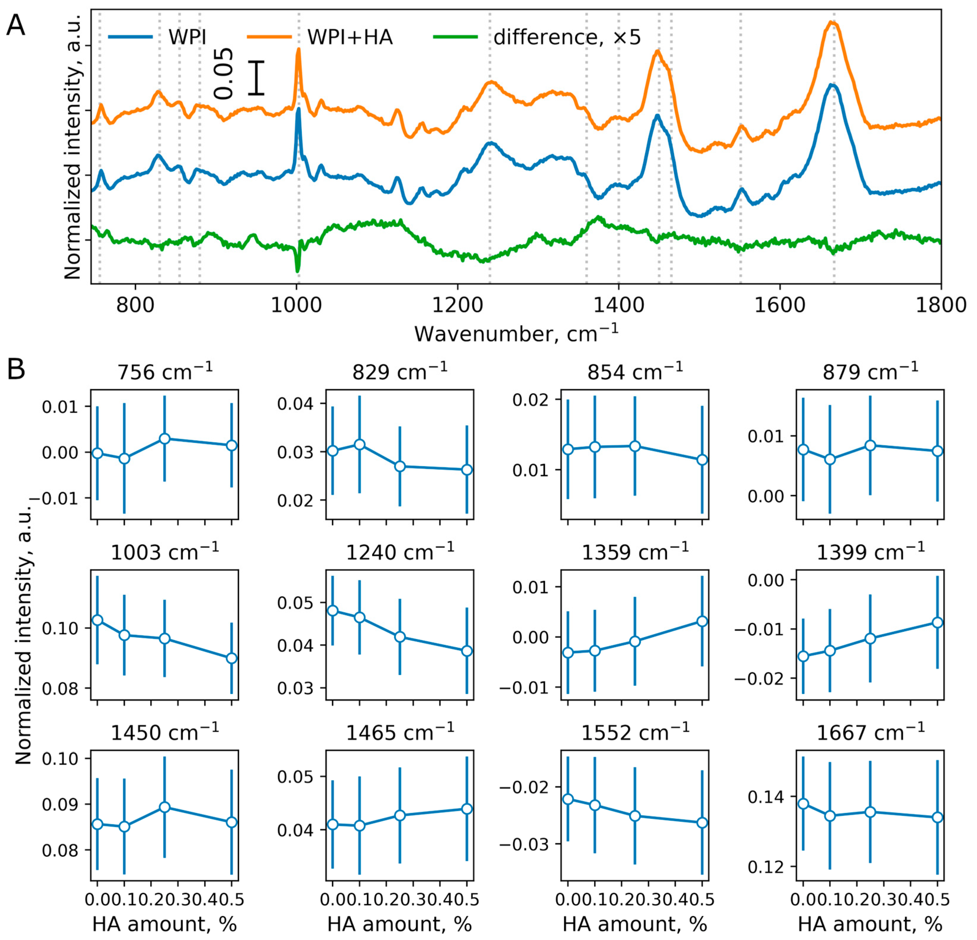
In order to analyze the impact of HA addition onto the chemical structure of WPI, three different conjugate compositions were prepared: WPI + 0.1% HA (5 wt.%:0.1 wt.%, 50:1 ratio), WPI + 0.25% HA (5 wt.%:0.25 wt.%, 20:1 ratio), WPI + 0.5% HA (5 wt.%:0.5 wt.%, 10:1 ratio). To further generalize the analysis process, WPIs were used from three different manufacturers (see Section 2.1). Thus, 12 different samples were prepared: three WPI sources; four HA amounts. Raman maps (20 × 10, 200 single spectra) were recorded for each WPI + HA conjugate as well as pure WPI (5 wt.%). The results of Raman spectroscopy are shown in Figure 1. All Raman bands of WPIs are indicated with gray dotted lines (Figure 1A).
There was only one Raman band at 1003 cm−1 on the difference spectrum (Figure 1A), on which the impact of HA addition can be noted. Normalized intensities of Raman bands marked on Figure 1A are shown in Figure 1B. Although there were trends in the mean intensities with respect to HA amounts, significant differences were not observed due to the high standard deviations (Figure 1B). Raman band assignments are indicated in Table 1.
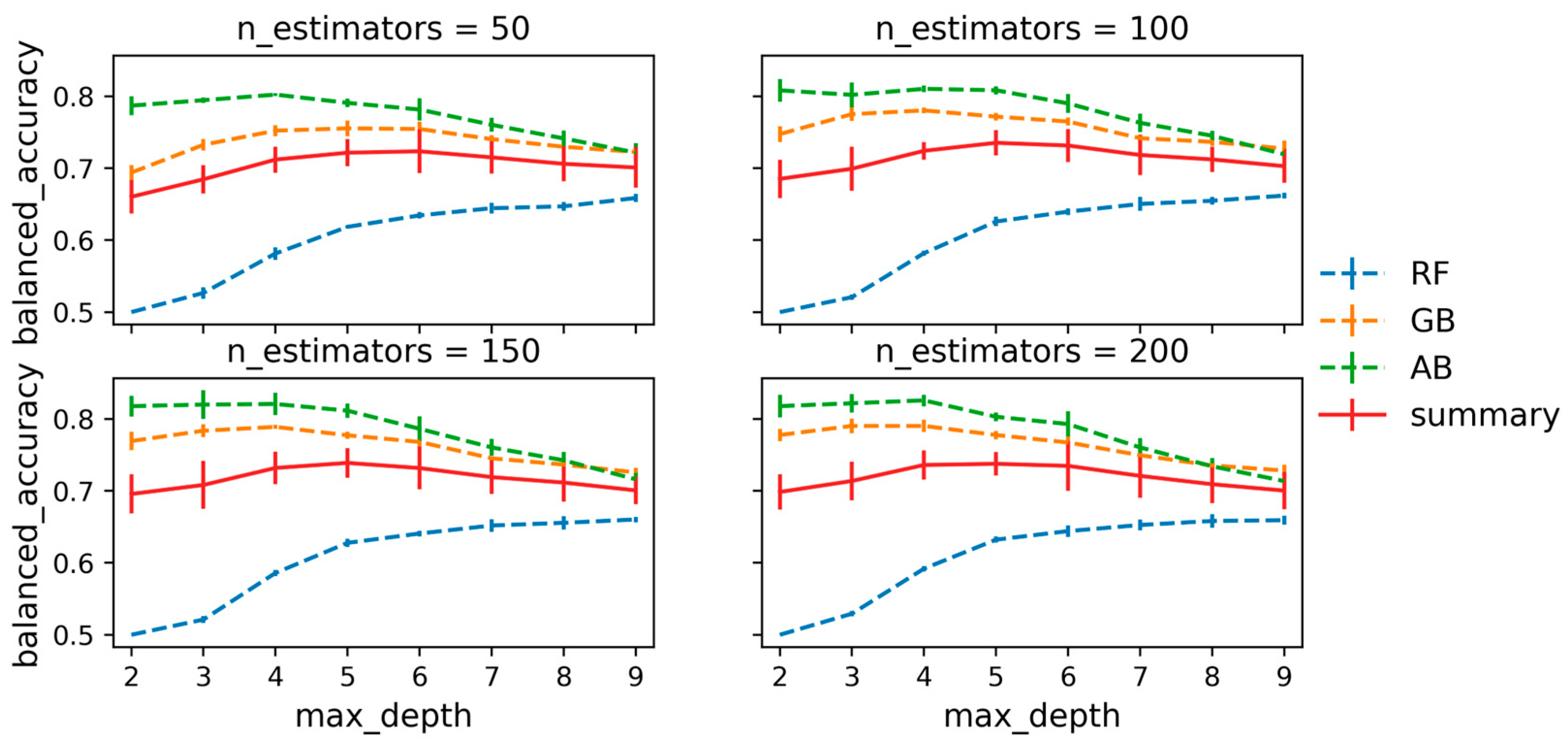
The conventional approach in analysis of Raman spectra (both by spectrum of difference and dependences of intensities on HA amount) has not provided a sufficient answer on which chemical bonds of WPIs changed the most upon HA addition and whether it is possible to reliably differentiate between WPI and WPI + HA. The latter can be crucial not only in the discussed conjugates but in considering wider issues of mixtures with small amounts of additives. To improve the analysis, the ensemble models based on DTs were implemented. Previously, RF, GB, and AB models were discussed [37,38]. In all of these models, DTs were used as individual estimators combined into an ensemble. As the current work is dedicated to a thorough analysis of the implementation of ensemble models to Raman spectroscopy data, Voting and Stacking models would also be discussed. To obtain higher performance of models, the number of DTs in the ensemble (n_estimators) and the maximum depth of each DT (max_depth) had been optimized using cross-validation via GridSearchCV [39,40] with balanced accuracy as a metric. The train dataset was divided into three subsets for cross-validation. Model metrics are shown in Figure 2. Summary (red line) indicates average metrics of RF, GB, and AB models.
Table 1. Raman bands of WPIs with their assignments [34,41,42,43].
Wavenumber, cm−1Assignment
756, 880, 1359Tryptophan, indole ring
830, 855Tyrosine, Fermi resonance between ring fundamental and overtone
1003Phenylalanine, ring breath
1125Rocking of NH3+
1206C–C stretching
1240Amide III (β-sheet), N–H in-plane bend, C–N stretch
1399Aspartic and glutamic acids, C=O stretch of COO–
1450, 1465Aliphatic residues, C–H bending
1552Tyrosine, ring stretching
1667Amide I, amide C=O stretch, N–H wag
The performance metric of classification models showed different behavior for bagging (RF) and boosting (GB, AB) algorithms (Figure 2). Presumably, boosting models with deep DTs were more prone to overfitting and, therefore, performed worse in the test dataset with an increasing max_depth. In contrast, an increase in the max_depth parameter led to an increase in the performance of the RF ensemble. For boosting models, there was also a slight increase in performance with an increase in max_depth up to 4. Thus, the optimal parameters for all models discussed were max_depth = 4 and n_estimators = 200. Balanced accuracies for all parameter combinations can be found in Table S1 (Supplementary Information).
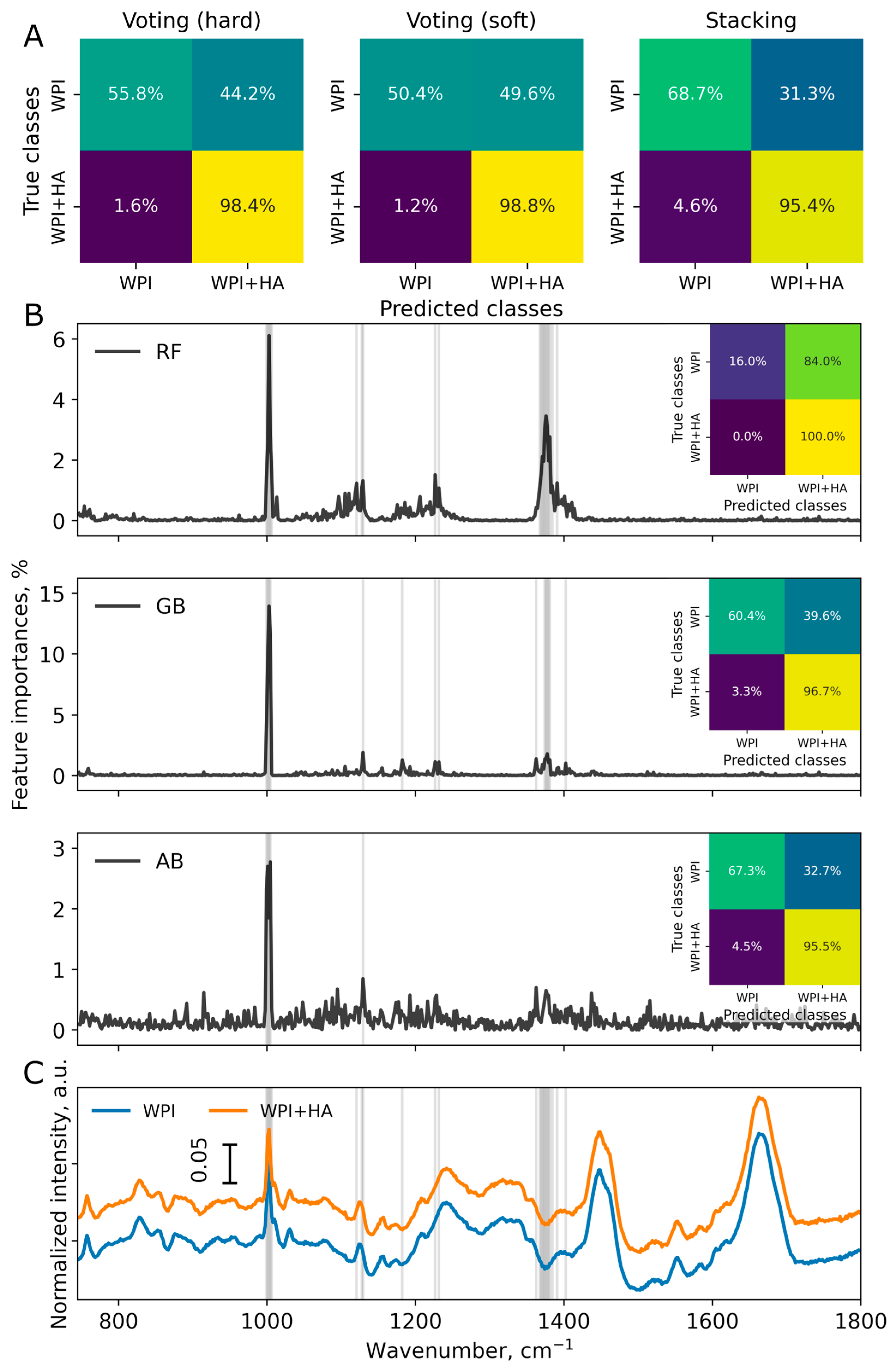
Six different classification models were compared: RF, GB, AB, Voting (hard), Voting (soft), and Stacking. In both Voting models, RF, GB, and AB were used as estimators, majority prognosis was implied in the hard version and average of class probabilities was used in the soft version. In Stacking, predictions of RF, GB, and AB were used as input data to the logistic regressor, which was applied as a final estimator in the ensemble. The following metrics were calculated to evaluate the performance of each model: confusion matrix, accuracy, sensitivity, and specificity. The results of the classification of WPI and WPI + HA Raman data are shown on Figure 3 and Figure S1 and in Table 2.
Classification models based on DT (namely, RF, GB, and AB) can also provide information on the importance of features. As intensities at different wavenumbers are considered as features in the analysis, this information can be visualized in the same wavenumber range as the Raman spectra being analyzed (Figure 3B). The classification model developed using the RF algorithm was determined to be less precise and less specified than the other models that were evaluated. Although WPI + HA spectra were correctly labeled by the RF model in 100% of the test dataset, 84.0% of the WPI spectra in the test dataset was also considered to be WPI + HA by the RF. Presumably, the lack of specificity observed could be due to the different sizes of the WPI and WPI + HA datasets used (a 1 to 3 ratio, as three different HA amounts were used for the WPI + HA data). Only wavenumbers with an importance to the analysis greater than 1% were considered valuable and were noted (Figure 3). The most important for RF, GB, and AB analyses were found to be 1003 cm−1 (ring breath of phenylalanine), 1125 cm−1 (rocking of NH3+), 1206 cm−1 (C–C stretching), and 1399 cm−1 (aspartic and glutamic acids, C=O stretch of COO–). As the dataset was biased in class sizes, the performance of classification models was limited by true negatives (correct prediction of WPI samples) and, thus, by model specificity. Considering this metric, the Stacking classifier was found to be the most effective model with a specificity of 0.687 (Table 2).
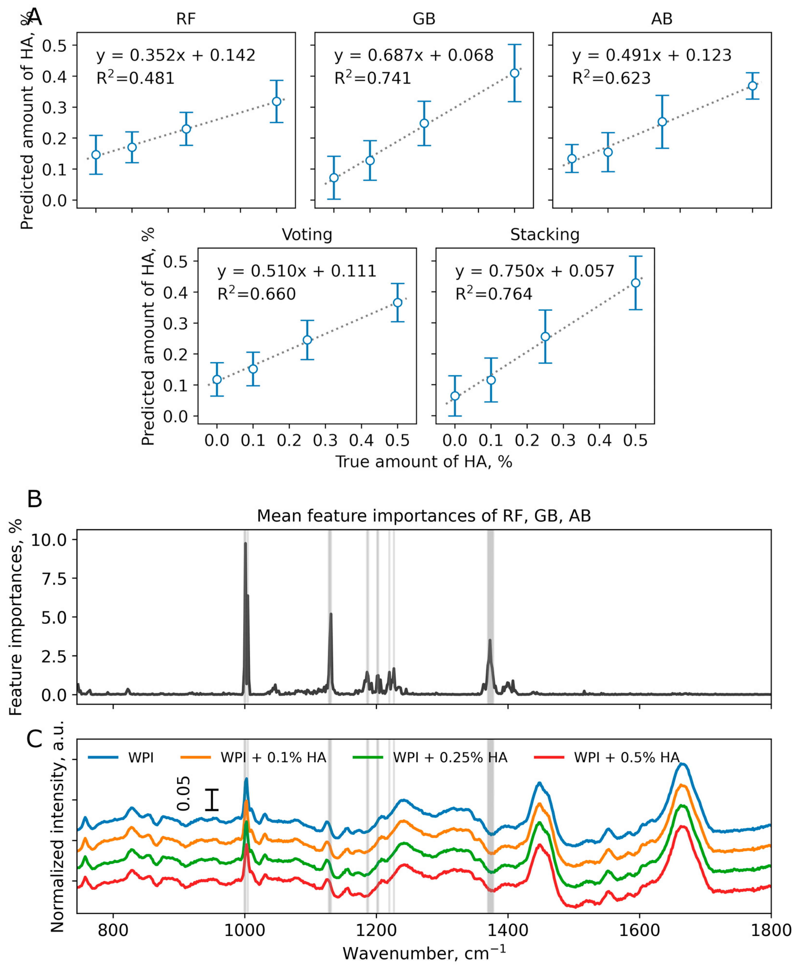
Although WPI samples could be distinguished from WPI + HA using classification models fitted to Raman spectroscopy data, other tasks remained equally important. Consequently, the possibility of creating regression models that could be used on the same dataset was also investigated. Five different regression models have been implemented, namely, RF, GB, AB, Voting, and Stacking. The additional model optimization had not been performed; the trained RF, GB, and AB regression models consisted of 200 DT with max_depth equal to 4. Similarly to the classification task, the Voting regressor generated the final prediction by averaging RF, GB, and AB results. In the Stacking regressor, the Ridge model with cross-validation utilized RF, GB, and AB prognoses as inputs. In the constructed regression task, the amount of HA in WPI + HA samples (0, 0.1, 0.25, and 0.5 wt.%) was used as the target value. The results of solving the regression task are demonstrated in Figure 4 and Figure S2 and Table 3. In order to evaluate the performance of each model, the R2 (determination coefficient) metric was applied.
According to feature importance plots, the wavenumbers with most impact on the regression models were found to be 1003 cm−1 (phenylalanine, ring breath), 1206 cm−1 (C–C stretching), 1125 cm−1 (rocking of NH3+), 1240 cm−1 (amide III (β-sheet), N–H in-plane bend, C–N stretch), and 1399 cm−1 (aspartic and glutamic acids, C=O stretch of COO–) (Figure S2). In most of the regression models discussed, all four spectra groups were clearly distinguishable. However, the best regression model for the discussed dataset was found to be the Stacking regressor (R2 = 0.764).
To further evaluate the generalization ability of the most promising model, leave-one-source-out cross-validation was performed for the Stacking algorithm (Table S2). Across the three manufacturers, the Stacking classifier achieved a balanced accuracy of 0.796 ± 0.111, while the Stacking regressor yielded an R2 of 0.733 ± 0.065. These results indicate that the model generalizes well to previously unseen protein sources.
Our results align with previous reports that employed tree-based ensemble methods for vibrational spectroscopy data. For instance, Sevetlidis and Pavlidis [14] achieved high classification accuracy for pigment identification using Random Forest on Raman spectra, while Wang and Zhang [19] applied Gradient Boosting to SERS data for Pb2+ detection. Compared to these studies, our work not only demonstrates the utility of Stacking and Voting ensembles but also provides a direct comparison between classification and regression tasks on the same dataset. Notably, the Stacking model outperformed individual classifiers, consistent with the principle that combining diverse base learners can reduce bias and variance [23]. Moreover, while traditional Raman difference spectroscopy (Figure 1A) revealed only subtle changes at 1003 cm−1, the feature importance maps of our models identified additional wavenumbers (1125, 1206, 1240, 1399 cm−1) that are critical for differentiation. This highlights the superior sensitivity of ensemble learning in detecting weak spectral variations that are invisible to conventional analysis.

4. Conclusions

A thorough analysis of the implementation of ensemble models in Raman spectroscopy data was performed. The dataset consisted of WPI (5 wt.%), WPI + 0.1% HA (5 wt.%:0.1 wt.%, 50:1 ratio), WPI + 0.25% HA (5 wt.%:0.25 wt.%, 20:1 ratio), and WPI + 0.5% HA (5 wt.%:0.5 wt.%, 10:1 ratio) Raman spectra (600 spectra per sample type). Additionally, these datasets were collected from three different WPI sources to achieve a more generalized result.
Classification models were used to answer the question of whether it is possible to detect differences between pure protein (WPI) and its conjugate with polysaccharide (WPI + HA). Prior to solving, Random Forest, Gradient Boosting, and AdaBoost models were optimized in the number of decision trees utilized and the maximum depth of each decision tree. The optimal parameters were evaluated using grid search with cross-validation and found to be 200 decision trees with a maximum depth of 4. Out of the six discussed models, namely Random Forest, Gradient Boosting, AdaBoost, Voting soft and hard, and Stacking, the latter performed the best with an overall accuracy of 82.0%, specificity of 68.7% and sensitivity of 95.4%. Moreover, RF, GB, and AB models provided additional information on the Raman bands of most importance in the obtained predictions: 1003 cm−1 (ring breath of phenylalanine), 1125 cm−1 (rocking of NH3+), 1206 cm−1 (C–C stretching), and 1399 cm−1 (aspartic and glutamic acids, C=O stretch of COO–).
Regression models were implemented not only to distinguish between Raman spectra of protein and its conjugate, but also to specifically determine the HA amount. The best model in solving the regression task was found to be the Stacking regressor, which utilized the Ridge model with cross-validation and RF, GB, and AB predictions as inputs. The determination coefficient of this model was found to be 0.764. RF, GB, and AB regression models had also determined additional importance in the analysis of the Raman band at 1240 cm−1 (amide III (β-sheet), N–H in-plane bend, C–N stretch).
The implementation of ensemble models in the analysis of Raman spectroscopy could be perceived as an intermediate solution between classical machine learning and neural networks. The training process of such models is less time consuming; however, the obtained performance is quite high. The discussed approach could be implemented in the analyses of various Raman spectroscopy data.
Despite the promising results, several limitations should be acknowledged. The model was trained and validated using spectra from three commercial WPI sources, but its effectiveness on other protein isolates or varying HA molecular weights has yet to be determined. Additionally, the spectral dataset was collected under controlled laboratory conditions; translation to real-world applications may require further adaptation. Future work will focus on validating the approach with a larger panel of independent samples, exploring deep learning architectures, and integrating the models into portable Raman devices for field use.

Supplementary Materials

The following supporting information can be downloaded at: https://www.mdpi.com/article/10.3390/macromol6020037/s1, Figure S1: ROC curves of RF, GB, AB, Voting (soft), and Stacking models with corresponding AUC values. Table S1: Balanced accuracies across 3 cross-validations of RF, GB, and AB models with different numbers of DTs (n_estimators) and maximum depth of each DT (max_depth). Parameters with the best average metrics across models are in bold. Figure S2: Feature importances of RF, GB, and AB regression models (black plots). Wavenumbers with importance greater than 1% are marked with vertical gray lines. Normalized mean spectra of WPI (blue line), WPI + 0.1% HA (orange line), WPI + 0.25% HA (green line), and WPI + 0.5% HA (red line). Spectra are offset for clarity. Table S2: Metrics of Stacking classification and regression models for leave-one-source-out cross-validation.

Author Contributions

Conceptualization, O.A.M. and E.S.P.; methodology, E.S.P.; software, S.A.S., S.A.G. and E.S.P.; validation, E.S.P.; formal analysis, E.S.P.; investigation, S.A.S., O.A.M., M.S.S. and E.S.P.; resources, E.S.P.; data curation, E.S.P.; writing—original draft preparation, E.S.P.; writing—review and editing, S.A.S., O.A.M., M.S.S. and E.S.P.; visualization, E.S.P.; supervision, E.S.P.; project administration, E.S.P.; funding acquisition, E.S.P. All authors have read and agreed to the published version of the manuscript.

Funding

This research was funded by the Russian Ministry of Science and Higher Education (state assignment no. FSMG-2025-0054).

Institutional Review Board Statement

Not applicable.

Data Availability Statement

The raw data supporting the conclusions of this article will be made available by the authors on request.

Conflicts of Interest

The authors declare no conflicts of interest.

Abbreviations

The following abbreviations are used in this manuscript:
ABAdaBoost
DTDecision tree
GBGradient boosting
HAHyaluronic acid
MAEMean absolute error
RMSERoot mean squared error
RFRandom forest
WPIWhey protein isolate

References

  1. Vaou, N.; Stavropoulou, E.; Voidarou, C.; Tsakris, Z.; Rozos, G.; Tsigalou, C.; Bezirtzoglou, E. Interactions between Medical Plant-Derived Bioactive Compounds: Focus on Antimicrobial Combination Effects. Antibiotics 2022, 11, 1014. [Google Scholar] [CrossRef]
  2. Mehta, N.; Kumar, P.; Verma, A.K.; Umaraw, P.; Kumar, Y.; Malav, O.P.; Sazili, A.Q.; Domínguez, R.; Lorenzo, J.M. Microencapsulation as a Noble Technique for the Application of Bioactive Compounds in the Food Industry: A Comprehensive Review. Appl. Sci. 2022, 12, 1424. [Google Scholar] [CrossRef]
  3. Senthilkumar, K.; Vijayalakshmi, A.; Jagadeesan, M.; Somasundaram, A.; Pitchiah, S.; Gowri, S.S.; Ali Alharbi, S.; Javed Ansari, M.; Ramasamy, P. Preparation of self-preserving personal care cosmetic products using multifunctional ingredients and other cosmetic ingredients. Sci. Rep. 2024, 14, 19401. [Google Scholar] [CrossRef]
  4. Saletnik, A.; Saletnik, B.; Puchalski, C. Overview of Popular Techniques of Raman Spectroscopy and Their Potential in the Study of Plant Tissues. Molecules 2021, 26, 1537. [Google Scholar] [CrossRef]
  5. Rebrosova, K.; Samek, O.; Kizovsky, M.; Bernatova, S.; Hola, V.; Ruzicka, F. Raman Spectroscopy—A Novel Method for Identification and Characterization of Microbes on a Single-Cell Level in Clinical Settings. Front. Cell. Infect. Microbiol. 2022, 12, 866463. [Google Scholar] [CrossRef]
  6. Pezzotti, G. Raman spectroscopy in cell biology and microbiology. J. Raman Spectrosc. 2021, 52, 2348–2443. [Google Scholar] [CrossRef]
  7. Kočišová, E.; Kuižová, A.; Procházka, M. Analytical applications of droplet deposition Raman spectroscopy. Analyst 2024, 149, 3276–3287. [Google Scholar] [CrossRef]
  8. Dodo, K.; Fujita, K.; Sodeoka, M. Raman Spectroscopy for Chemical Biology Research. J. Am. Chem. Soc. 2022, 144, 19651–19667. [Google Scholar] [CrossRef]
  9. Koronaki, E.D.; Kaven, L.F.; Faust, J.M.M.; Kevrekidis, I.G.; Mitsos, A. Nonlinear manifold learning determines microgel size from Raman spectroscopy. AIChE J. 2024, 70, e18494. [Google Scholar] [CrossRef]
  10. Zhang, Y.; Gao, P.; Zhang, N.; Hong, H.; Ruan, J.; Gao, X. Efficient detection of specific pharmaceutical components in compound medications based on Raman spectroscopy. Opt. Commun. 2025, 577, 131470. [Google Scholar] [CrossRef]
  11. Sun, Y.; Tang, H.; Zou, X.; Meng, G.; Wu, N. Raman spectroscopy for food quality assurance and safety monitoring: A review. Curr. Opin. Food Sci. 2022, 47, 100910. [Google Scholar] [CrossRef]
  12. Becker, T.; Rousseau, A.-J.; Geubbelmans, M.; Burzykowski, T.; Valkenborg, D. Decision trees and random forests. Am. J. Orthod. Dentofac. Orthop. 2023, 164, 894–897. [Google Scholar] [CrossRef] [PubMed]
  13. da Silva, L.P.; Oliveira, M.D.L.; Villa, J.E.L. A comparison of decision tree-based algorithms for food discrimination using vibrational spectroscopy. Food Chem. 2025, 488, 144909. [Google Scholar] [CrossRef]
  14. Sevetlidis, V.; Pavlidis, G. Effective Raman spectra identification with tree-based methods. J. Cult. Herit. 2019, 37, 121–128. [Google Scholar] [CrossRef]
  15. Sun, Z.; Wang, G.; Li, P.; Wang, H.; Zhang, M.; Liang, X. An improved random forest based on the classification accuracy and correlation measurement of decision trees. Expert Syst. Appl. 2024, 237, 121549. [Google Scholar] [CrossRef]
  16. Breiman, L. Random Forests. Mach. Learn. 2001, 45, 5–32. [Google Scholar] [CrossRef]
  17. Friedman, J.H. Greedy Function Approximation: A Gradient Boosting Machine. Ann. Stat. 2001, 29, 1189–1232. [Google Scholar] [CrossRef]
  18. Friedman, J.H. Stochastic gradient boosting. Comput. Stat. Data Anal. 2002, 38, 367–378. [Google Scholar] [CrossRef]
  19. Wang, M.; Zhang, J. Surface Enhanced Raman Spectroscopy Pb2+ Ion Detection Based on a Gradient Boosting Decision Tree Algorithm. Chemosensors 2023, 11, 509. [Google Scholar] [CrossRef]
  20. Freund, Y.; Schapire, R.E. A Decision-Theoretic Generalization of On-Line Learning and an Application to Boosting. J. Comput. Syst. Sci. 1997, 55, 119–139. [Google Scholar] [CrossRef]
  21. Zhu, J.; Zou, H.; Rosset, S.; Hastie, T. Multi-class adaboost. Stat. Interface 2009, 2, 349–360. [Google Scholar]
  22. Dietterich, T.G. Ensemble Methods in Machine Learning. In International Workshop on Multiple Classifier Systems; Springer: Berlin/Heidelberg, Germany, 2000; pp. 1–15. [Google Scholar]
  23. Wolpert, D.H. Stacked generalization. Neural Netw. 1992, 5, 241–259. [Google Scholar] [CrossRef]
  24. Bates, F.; Busato, M.; Piletska, E.; Whitcombe, M.J.; Karim, K.; Guerreiro, A.; del Valle, M.; Giorgetti, A.; Piletsky, S. Computational design of molecularly imprinted polymer for direct detection of melamine in milk. Sep. Sci. Technol. 2017, 52, 1441–1453. [Google Scholar] [CrossRef]
  25. Lu, Y.; Xia, Y.; Liu, G.; Pan, M.; Li, M.; Lee, N.A.; Wang, S. A Review of Methods for Detecting Melamine in Food Samples. Crit. Rev. Anal. Chem. 2017, 47, 51–66. [Google Scholar] [CrossRef] [PubMed]
  26. Niazifar, M.; Besharati, M.; Jabbar, M.; Ghazanfar, S.; Asad, M.; Palangi, V.; Eseceli, H.; Lackner, M. Slow-release non-protein nitrogen sources in animal nutrition: A review. Heliyon 2024, 10, e33752. [Google Scholar] [CrossRef]
  27. Alizadeh Sani, M.; Jahed-Khaniki, G.; Ehsani, A.; Shariatifar, N.; Dehghani, M.H.; Hashemi, M.; Hosseini, H.; Abdollahi, M.; Hassani, S.; Bayrami, Z.; et al. Metal–Organic Framework Fluorescence Sensors for Rapid and Accurate Detection of Melamine in Milk Powder. Biosensors 2023, 13, 94. [Google Scholar] [CrossRef]
  28. Lukacs, M.; Zaukuu, J.-L.Z.; Bazar, G.; Pollner, B.; Fodor, M.; Kovacs, Z. Comparison of Multiple NIR Spectrometers for Detecting Low-Concentration Nitrogen-Based Adulteration in Protein Powders. Molecules 2024, 29, 781. [Google Scholar] [CrossRef]
  29. Lukacs, M.; Bazar, G.; Pollner, B.; Henn, R.; Kirchler, C.G.; Huck, C.W.; Kovacs, Z. Near infrared spectroscopy as an alternative quick method for simultaneous detection of multiple adulterants in whey protein-based sports supplement. Food Control 2018, 94, 331–340. [Google Scholar] [CrossRef]
  30. Marinho, A.; Nunes, C.; Reis, S. Hyaluronic Acid: A Key Ingredient in the Therapy of Inflammation. Biomolecules 2021, 11, 1518. [Google Scholar] [CrossRef] [PubMed]
  31. Yasin, A.; Ren, Y.; Li, J.; Sheng, Y.; Cao, C.; Zhang, K. Advances in Hyaluronic Acid for Biomedical Applications. Front. Bioeng. Biotechnol. 2022, 10, 910290. [Google Scholar] [CrossRef]
  32. Juncan, A.M.; Moisă, D.G.; Santini, A.; Morgovan, C.; Rus, L.-L.; Vonica-Țincu, A.L.; Loghin, F. Advantages of Hyaluronic Acid and Its Combination with Other Bioactive Ingredients in Cosmeceuticals. Molecules 2021, 26, 4429. [Google Scholar] [CrossRef]
  33. Iaconisi, G.N.; Lunetti, P.; Gallo, N.; Cappello, A.R.; Fiermonte, G.; Dolce, V.; Capobianco, L. Hyaluronic Acid: A Powerful Biomolecule with Wide-Ranging Applications—A Comprehensive Review. Int. J. Mol. Sci. 2023, 24, 10296. [Google Scholar] [CrossRef]
  34. Wang, N.; Zhao, X.; Jiang, Y.; Ban, Q.; Wang, X. Enhancing the stability of oil-in-water emulsions by non-covalent interaction between whey protein isolate and hyaluronic acid. Int. J. Biol. Macromol. 2023, 225, 1085–1095. [Google Scholar] [CrossRef]
  35. Henderson, A. Renishaw File Reader. 2017. Available online: https://zenodo.org/records/495477 (accessed on 25 November 2025).
  36. Pedregosa, F.; Varoquaux, G.; Gramfort, A.; Michel, V.; Thirion, B.; Grisel, O.; Blondel, M.; Prettenhofer, P.; Weiss, R.; Dubourg, V.; et al. Scikit-learn: Machine Learning in Python. J. Mach. Learn. Res. 2011, 12, 2825–2830. [Google Scholar]
  37. Mayorova, O.A.; Saveleva, M.S.; Bratashov, D.N.; Prikhozhdenko, E.S. Combination of Machine Learning and Raman Spectroscopy for Determination of the Complex of Whey Protein Isolate with Hyaluronic Acid. Polymers 2024, 16, 666. [Google Scholar] [CrossRef] [PubMed]
  38. Shevtsova, S.A.; Saveleva, M.S.; Mayorova, O.A.; Prikhozhdenko, E.S. Effect of low concentrations of hyaluronic acid on the structure of whey protein isolate during conjugation: Development and optimization of machine learning models based on adaptive boosting for spectroscopic data analysis. Izv. Saratov Univ. Phys. 2025, 25, 305–315. [Google Scholar] [CrossRef]
  39. Kurniasih, A.; Previana, C.N. Implementation of GridSearchCV to Find the Best Hyperparameter Combination for Classification Model Algorithm in Predicting Water Potability. J. Artif. Intell. Eng. Appl. 2025, 4, 1174–1182. [Google Scholar] [CrossRef]
  40. Muzayanah, R.; Pertiwi, D.A.A.; Ali, M.; Muslim, M.A. Comparison of gridsearchcv and bayesian hyperparameter optimization in random forest algorithm for diabetes prediction. J. Soft Comput. Explor. 2024, 5, 86–91. [Google Scholar] [CrossRef]
  41. Zhang, S.; Zhang, Z.; Lin, M.; Vardhanabhuti, B. Raman Spectroscopic Characterization of Structural Changes in Heated Whey Protein Isolate upon Soluble Complex Formation with Pectin at Near Neutral pH. J. Agric. Food Chem. 2012, 60, 12029–12035. [Google Scholar] [CrossRef]
  42. Zhao, Y.; Ma, C.-Y.; Yuen, S.-N.; Phillips, D.L. Study of Succinylated Food Proteins by Raman Spectroscopy. J. Agric. Food Chem. 2004, 52, 1815–1823. [Google Scholar] [CrossRef]
  43. Zhu, G.; Zhu, X.; Fan, Q.; Wan, X. Raman spectra of amino acids and their aqueous solutions. Spectrochim. Acta A Mol. Biomol. Spectrosc. 2011, 78, 1187–1195. [Google Scholar] [CrossRef] [PubMed]
Figure 1. Raman spectroscopy data on WPI and WPI + n% HA (n = 0.1, 0.25, 0.5). (A) Average spectra of WPI (1800 spectra) and WPI + HA (1800 spectra per HA amount; 5400 spectra overall). Raman bands of WPI marked with gray dotted lines. Spectrum of difference was magnified by 5 for clarity. (B) Dependence of Raman band normalized intensities on HA amount (mean ± standard deviation, n = 1800 spectra per HA amount).
Macromol 06 00037 g001
Figure 2. Accuracies of RF, GB, and AB models on maximum depth (max_depth) and number of DTs (n_estimators). Summary represents average metrics of RF, GB, and AB models. Mean values and standard deviations were calculated in cross-validation (n = 3).
Macromol 06 00037 g002
Figure 3. (A) Confusion matrices of Voting classifiers (hard and soft) and Stacking classifier; test dataset consists of 450 spectra of WPI and 1350 spectra of WPI + HA (450 spectra per each HA amount: 0.1, 0.25, and 0.5 wt.%). (B) Mean feature importances of RF, GB, and AB with corresponding confusion matrices. Wavenumbers with importance greater than 1% are marked with vertical gray lines. (C) Normalized mean spectra of WPI and WPI + HA.
Macromol 06 00037 g003
Figure 4. (A) Linear regression plots between true and predicted HA amounts calculated for test dataset (450 spectra per HA amount). Corresponding regression equations with R2 values are indicated for each regression model. (B) Mean feature importances of RF, GB, and AB. Wavenumbers with importance greater than 1% are marked with vertical gray lines. (C) Normalized mean spectra of WPI, WPI + 0.1% HA, WPI + 0.25% HA, and WPI + 0.5% HA. Spectra are offset for clarity.
Macromol 06 00037 g004
Table 2. Metrics of classification models.
Model\MetricRFGBABVoting (Hard)Voting (Soft)Stacking
Balanced Accuracy0.5800.7860.8140.7710.7460.820
Precision0.7810.8800.8980.8700.8570.901
Recall1.0000.9670.9550.9840.9880.954
F1 score0.8770.9220.9250.9230.9180.927
Sensitivity1.0000.9670.9550.9840.9880.954
Specificity0.1600.6040.6730.5580.5040.687
Table 3. Metrics of regression models.
Model\MetricRFGBABVoting (Hard)Stacking
MAE0.1110.0700.0990.0890.068
RMSE0.1350.0950.1150.1100.091
R20.4810.7410.6230.6600.764
Disclaimer/Publisher’s Note: The statements, opinions and data contained in all publications are solely those of the individual author(s) and contributor(s) and not of MDPI and/or the editor(s). MDPI and/or the editor(s) disclaim responsibility for any injury to people or property resulting from any ideas, methods, instructions or products referred to in the content.